Article

Can We Use Machine Learning for Agricultural Land Suitability Assessment?

by
Anders Bjørn Møller
1,*,
Vera Leatitia Mulder
2,
Gerard B. M. Heuvelink
2,
Niels Mark Jacobsen
1 and
Mogens Humlekrog Greve
1
1
Department of Agroecology, Aarhus University, Blichers Allé 20, 8830 Tjele, Denmark
2
Soil Geography and Landscape Group, Wageningen University and Research, P.O. Box 47, 6700 AA Wageningen, The Netherlands
*
Author to whom correspondence should be addressed.
Agronomy 2021, 11(4), 703; https://doi.org/10.3390/agronomy11040703
Submission received: 26 February 2021 / Revised: 31 March 2021 / Accepted: 2 April 2021 / Published: 7 April 2021
(This article belongs to the Special Issue Machine Learning Applications in Digital Agriculture)

Abstract

:
It is vital for farmers to know if their land is suitable for the crops that they plan to grow. An increasing number of studies have used machine learning models based on land use data as an efficient means for mapping land suitability. This approach relies on the assumption that farmers grow their crops in the best-suited areas, but no studies have systematically tested this assumption. We aimed to test the assumption for specialty crops in Denmark. First, we mapped suitability for 41 specialty crops using machine learning. Then, we compared the predicted land suitabilities with the mechanistic model ECOCROP (Ecological Crop Requirements). The results showed that there was little agreement between the suitabilities based on machine learning and ECOCROP. Therefore, we argue that the methods represent different phenomena, which we label as socioeconomic suitability and ecological suitability, respectively. In most cases, machine learning predicts socioeconomic suitability, but the ambiguity of the term land suitability can lead to misinterpretation. Therefore, we highlight the need for increasing awareness of this distinction as a way forward for agricultural land suitability assessment.

1. Introduction

Farmers face many risks in the form of adverse weather, pests, diseases, and changes in crop prices, laws, and regulations [1,2,3]. A first step in managing and minimizing many of these risks is often to select appropriate crops for the cultivated areas. Therefore, knowing if the land is suitable for a specific crop can decide the success or failure of agricultural strategies. As farmers are subject to climate change and a globalized economy, where frameworks for agriculture change at unprecedented speed, it is vital for them to be able to adapt to new trends [4,5,6]. Increasing the availability of land suitability information for agricultural crops would be a valuable aid for farmers to devise new agricultural strategies. At the same time, growing computational capabilities and the increasing availability of geographic data have made it quicker and easier to conduct land suitability assessments.
Conventional land suitability assessment, also known as land evaluation, is mainly a tool for land use planning in local or national governments [7]. As such, in most cases, it has relied on qualitative evaluation of the societal benefits of different land uses [7,8], and in recent years, it has increasingly incorporated environmental aspects [9]. The Food and Agriculture Organization of the United Nations (FAO) developed a formalized approach to land evaluation [7], and ref. [10] elaborated a theoretical framework for land evaluation. In practice, land evaluation has made use of widely different methods. Studies may focus on the climate [11,12] or the soil [13,14], and they may include socioeconomic variables [15,16].
Other approaches to land suitability assessment include crop growth models [17,18,19] and human–environment land systems models [20]. Land systems models mainly serve to explore and predict the socioeconomic dynamics of land use change [21,22], but they can also produce maps of land suitability for specific crops [23]. Land evaluation, crop growth models, and land systems models share a strong reliance on expert knowledge and large investments of time. This has created a growing interest in automatable methods, such as mechanistic crop models [24]. One of the most frequently applied mechanistic methods used in land suitability assessment is the ECOCROP (Ecological Crop Requirements) model [25,26,27,28,29,30,31,32], which is based on the ECOCROP database [33].
Machine learning (ML) models based on land use patterns are another widespread automated method for land suitability assessment. ML is a sub-field of computer science, closely related to statistics, which aims to make computers learn from data without explicit programming [34]. As such, ML uses data-driven inductive models, unlike the previously mentioned deductive approaches. ML has gained widespread use in soil mapping [35,36], species distribution modeling [37,38], land use mapping, and land cover classification [39]. The most common ML approach to land suitability assessment relies on models trained with the Maxent algorithm using all the available land use data with no socioeconomic covariates [40,41,42,43,44,45,46]. This approach builds on the assumption that farmers cultivate crops in the areas where they have the best growing conditions [47]. Some studies have shown results that contradict this assumption [48,49], but no studies have systematically tested it. Furthermore, ML differs very much from ECOCROP. While ECOCROP focuses on ecological crop requirements, ML can potentially use any variable that researchers deem relevant, including socioeconomic variables [23,48,50]. In addition, ML is a data-driven approach that aims to reproduce observed patterns, whereas ECOCROP defines the suitable growing conditions a priori. Despite these dissimilarities, comparisons between the methods are rare, and the relationship between the suitabilities that they produce remains unclear. In this study, we aim to elucidate and discuss this connection by comparing land suitability maps produced with Maxent to maps based on ECOCROP for different specialty crops in Denmark. We use specialty crops because a substantial number of earlier studies have focused on this category [44,45,46,51,52,53]. Furthermore, yield data are often not systematically available for specialty crops, and the quality of the produce may be more important than the yield [54,55]. Therefore, yield does not always reflect the value of the produce, which makes ML an attractive alternative for land suitability assessment. We will compare the ML models, their accuracies, and covariate usage to ECOCROP suitability maps. We will use these results as a basis for exploring and discussing the meaning of the term land suitability, its relationship to land use, and how this affects ML as a means to map land suitability. As ML and ECOCROP are radically different approaches to land suitability assessment, we hypothesize that the two methods will yield different results and elucidate different aspects of land suitability. Where possible, we will also compare the results to the land use in 1896 to see how the suitabilities mapped with the two different methods relate to land use changes. Danish agriculture underwent radical changes in the 20th century, with increased mechanization, larger, more specialized farms, increased livestock densities, and larger amounts of external inputs in the form of fertilizers, pesticides, and imported feedstuffs [56]. Therefore, we also hypothesize that the land suitabilities based on ecological crop requirements will align more closely with land use in 1896 than the present land use. Finally, based on these comparisons, we will delineate possible ways forward for agricultural land suitability assessment.

2. Materials and Methods

2.1. Overview

We aimed to compare land suitability maps for all specialty crops with sufficient land use data using the ML algorithm Maxent and the mechanistic model ECOCROP (Figure 1). Supplementary Table S1 lists the investigated crops. Firstly, we trained Maxent models based on farmers’ crop registrations and various ancillary information and used these models to predict land suitability for the crops. Secondly, we produced ECOCROP suitability maps based on values from the ECOCROP database. We calculated accuracies for both sets of maps using the same holdout land use observations. We also calculated the rank correlations between the maps for each crop and compared the correlation with the predictive accuracies of the maps. Lastly, we conducted a visual comparison between the suitability maps for potatoes and carrots as well as historic land use maps for these two crops.

2.2. Study Area

Denmark, located in northern Europe, consists of the Jutland peninsula (29,778 km2) and several islands, the largest of which is Zealand (7031 km2) (Figure 2). Agricultural areas cover 61% of the country [57]. The country has a temperate coastal climate with temperatures ranging from 1 °C in January to 17 °C in July [58]. Mean annual precipitation ranges from 650 mm in the eastern parts of the country to 850 mm in the western parts of the country [58]. In the western parts of the country, the naturally occurring soils are mainly Podzols formed on sandy glaciofluvial outwash plains and Saalian moraines [59]. In the eastern parts, the most common natural soil types are Cambisols and Luvisols formed on loamy Weichselian till [59]. However, continued agricultural additions of calcium carbonates and animal manure have transformed many of these soils into Phaeozems [60,61].

2.3. Maxent Models

2.3.1. Training Data

We used farmers’ crop registrations for the Common Agricultural Policy of the European Union as training data for Maxent models to map land suitability [62]. We used registrations from the years 2011–2019, which are available as polygon data, showing the crops grown in individual fields. The combined area of the data was 28,077 km2. We used the definition of specialty crops of the US Department of Agriculture [63] to select 63 specialty crops from the farmers’ registrations. Next, we omitted specialty crops that did not have at least 30 registrations in at least one year. This narrowed our selection to 41 target specialty crops (Supplementary Table S1). Within this set of crops, we chose to emphasize two crops as examples to illustrate differences in land use and land suitability: Table potatoes (Solanum tuberosum) and carrots (Daucus carota subsp. Sativus). However, we used all 41 specialty crops for the overall analyses.
We converted the polygons from each year to rasters with 30.4 m × 30.4 m resolution to match existing soil maps and covariates for spatial predictions [61,64,65,66,67,68]. We randomly sampled raster cells with the crop for each year and for each target crop. We limited the number of training points for each crop to a maximum of 1500 cells per year in order to make the datasets computationally manageable. We also selected a matching number of absence points as a random sample of areas with other crops for each target crop in each year. In principle, Maxent can function without explicit absence data. However, Maxent achieves this by extracting a random background sample from the covariate layers [69]. Our covariates comprised the full area of Denmark, so we used an explicit background sample to avoid occurrences of urban areas and natural vegetation in the background data. Furthermore, our target crops were all relatively rare (<1% of the agricultural area in any given year), so there was only little difference between a background sample and absence data. Lastly, the absence data were useful for model evaluation, as researchers should evaluate their data in a presence/absence framework when it is possible [70].

2.3.2. Covariates

We employed 30 soil-related covariates, 14 climatic, 9 topographical, and 2 socioeconomic covariates (Supplementary Table S2). The soil-related covariates included contents of clay, silt, fine sand, coarse sand [65], and soil organic matter [64] in three depth intervals (0–30 cm, 30–60 cm, 60–100 cm). They also included plant-available water, pH, and bulk density [66] in the same three intervals, the phosphorus sorption capacity in four 25-cm depth intervals [71], the soil drainage class [68], and the geology at 1 m depth [72]. The climatic variables included eight bioclimatic variables from the WordClim 2 dataset [73], the number of degree days above 5 °C calculated from the same dataset, four agroclimatic variables from [74], and potential incoming solar radiation calculated based on a DEM. The topographical variables included a digital elevation model (DEM) [75], and derived variables including the slope gradient, the sine and cosine of the surface aspect, the topographical wetness index, the SAGA GIS wetness index, the relative slope position, the valley depth, and a map of landscape elements [76]. Lastly, the socioeconomic covariates comprised the Euclidean distances to cities with populations sizes of at least 10,000 and 100,000, respectively, based on data from the GeoDanmark data collection [77]. We converted the categorical variables geology and landscape elements to binary indicator variables, with one variable for each class in the original layers. This gave a final number of 74 covariates. Although we used land use observations from several years, we used the same covariates for the whole period. Some of the covariates, such as climatic covariates, may vary over the period, but we regarded them as static for the purpose of this study, as we mainly aimed to map general geographic patterns.

2.3.3. Models and Predictions

The used Maxent to produce maps of land suitability for each crop. We chose Maxent, as it is the most frequently used ML algorithm for mapping land suitability [40,41,42,43,44,45,46,47,48,49,53,78,79,80], although a few studies have applied other algorithms [49,50,52,80]. Researchers in ecology originally developed Maxent as a species distribution model, using environmental variables as inputs [81]. In land suitability assessment, most studies using Maxent have adopted similar methodologies.
Maxent is an additive algorithm that aims to model a logistic probability distribution. The algorithm sequentially adds features to the model, starting with the features with the largest information gain. Feature types include linear, quadratic, product (combining two covariates), threshold, hinge (combining linear and threshold), and categorical features [81,82]. The available feature types depend on the number of presence points, but with more than 100 presence points, all feature types are available [83]. Maxent also includes built-in regularization to reduce overfitting. The regularization includes penalization for complex features with penalization parameters (β) that depend on the feature type and the number of presence points [81]. With more than 100 presence points, the default β is 0.05 for linear, quadratic, and product features, 0.25 for categorical features, 0.50 for hinge features, and 1.00 for threshold features [83]. Furthermore, Maxent divides β by the square root of the number of presence points, allowing larger complexity with larger sample sizes. Users can specify which feature types to include and choose to modify regularization by multiplying the default β with a factor [82]. By default, Maxent will add features to the model until there is no information gain or until a maximum of 500 features [83].
We trained a Maxent model for each target crop using the function maxent from the R package dismo [84]. In all cases, we used the default parameters decided by Maxent based on the number of training observations. In practice, this means that all feature types were available, we did not modify β, and the models contained up to 500 features. While adjusting the parameters can potentially increase predictive accuracies, Maxent can often achieve acceptable accuracies with the default settings [81]. Then, we used the resulting models to produce maps of land suitability for each crop. Maxent treats suitability as a continuous variable from 0 (fully unsuitable) to 1 (optimally suited).
We assessed model accuracy for the Maxent models with a spatiotemporal cross-validation scheme. We chose this scheme for two reasons: Firstly, we wanted to avoid situations wherein observations from the same farm were present in the training dataset as well as the dataset for accuracy assessment. Secondly, we aimed to map general geographic patterns in land suitability, producing only one map with each model for each crop. Therefore, the predictions based on data from one year should also be accurate in other years. The scheme randomly selected 100 observations from a given year for accuracy assessment. Then, it eliminated all training observations from the same year and all training observations within a 10-km radius. Therefore, the accuracy assessment used models trained on observations from different years than the holdout observations and from locations substantially removed from them in geographic space. We repeated the process four times for each year for each crop. The accuracy assessment scheme is generally similar to the Leave-Location-and-Time-out cross-validation scheme proposed by [85], with an addition of buffers around the hold-out observations in a manner similar to the function represampling_disc_bootstrap from the R package sperrorest [86]. We developed the specific code used in this study to combine these approaches.
We evaluated the accuracy of the predicted suitability values based on the overall accuracy (fraction of observations correctly predicted, OA) and the area under the receiver operator characteristic curve (AUC). We calculated AUC using the function roc from the R package pROC [87]. We calculated OA and AUC separately for all repetitions and used the mean value for each metric across all repetitions.
The maxent function automatically calculates the importance of the covariates by perturbation. The function randomly permutes the covariates one at a time and calculates the resulting decrease in AUC. We scaled importance to 100 for the most important covariate in each model and calculated the mean importance across all models.

2.4. ECOCROP

In order to compare the land suitabilities mapped with Maxent to land suitabilities based on ecological crop requirements, we used ECOCROP to produce maps of land suitability. We mainly chose ECOCROP due to its frequent application in land suitability assessment [25,26,27,28,29,30,31,32]. ECOCROP works by comparing maps of climatic variables to the temperature and precipitation thresholds listed for the crops in the database [26]. Although ECOCROP by default uses thresholds from the database as inputs, some studies have calibrated the values based on land use data [26,28]. Furthermore, while the default method includes only temperatures and precipitation, some studies have modified it to include soil properties [25,28,29,30] and topography [29,30]. Most studies using ECOCROP have focused on changes in land suitability under climate change scenarios [25,26,27,28,29,31,32].
ECOCROP calculates a suitability index between 0 and 1 for temperature and precipitation based on the optimal and absolute listed ranges for the crop [26]. Values inside the optimal range give an index of 1, values outside the absolute range give an index of 0, and values between the absolute and optimal ranges give a value interpolated between 0 and 1. ECOCROP calculates the temperature index on a monthly basis, excluding months where the minimum temperature is below the killing temperature for the crop, and it calculates a mean index for different potential growing seasons, taking into account the minimum and maximum lengths of the growing season required for the crop. Then, it calculates the precipitation index based on the total precipitation in each of the potential growing seasons and calculates the suitability as the product (multiplication) of the temperature and precipitation indices. The final suitability score is the highest score obtained for the potential growing season.
The ECOCROP database [33] lists crop requirements for a long list of environmental properties, but we focused on temperature, precipitation, soil pH, texture, and drainage, as experience has shown that these are some of the most important properties for crop yields in Denmark, e.g., [88]. Supplementary Table S1 lists the corresponding crops in the ECOCROP database for the target crops. The match between the Danish farmers’ registrations and the ECOCROP database is sometimes imperfect. For example, the database lists only one crop for cabbages (Brassica oleracea), whereas the farmers’ registrations list several varieties.
For each of the crops selected from the ECOCROP database, we first calculated climatic suitability (SC) using minimum and mean monthly temperatures and mean monthly precipitation from the WorldClim 2 dataset [73] using the function ecocrop from the R package dismo [84]. Then, we calculated suitabilities based on soil pH (SpH), texture (ST), and drainage (SD) for the crops based on maps of soil pH [66], the FAO soil texture classes [61], soil drainage classes [68], and artificially drained areas [67]. For soil pH, the ECOCROP database provides optimal and absolute ranges for suitability in a manner similar to temperature and precipitation. Therefore, we interpolated pH-related suitability between 0 for unsuitable areas and 1 for optimal areas. However, for soil texture and drainage, the database uses a number of classes that are either unsuitable, suitable, or optimally suited. In these maps, we assigned suitability values of 1 to optimally suited areas, 0.5 to suitable areas, and 0 to unsuitable areas. Table 1 gives examples of these suitability values as well as the optimal and absolute ranges for temperature, precipitation and soil pH listed in the database for the two focus crops: potatoes and carrots. Supplementary Tables S3 and S4 list the climatic and soil-related requirements for each crop in the study, according to the ECOCROP database.
We produced ECOCROP suitability maps for each crop, which were calculated as the product of the climatic, soil pH, textural, and drainage suitabilities:
SE = SC ∙ SpH ∙ ST ∙ SD,
where SE is the ECOCROP suitability.
Elder (Sambucus nigra) and rosehip (Rosa rogusa) had no corresponding crops in the ECOCROP database, and we therefore produced no suitability maps for these two crops. We compared the ECOCROP suitability maps to the maps produced with Maxent by calculating Spearman’s rank correlation coefficient ρ between the maps for each crop. We also calculated OA and AUC for the ECOCROP suitability maps using the same observations that we used for assessing the accuracy of the Maxent models.

2.5. Historic Land Use Data

We compared the suitability maps produced with Maxent and ECOCROP to historic land use for the two focus crops (table potatoes and carrots). Specifically, we used land use data collected at the parish level for the year 1896. We obtained the land use data from a historical tabular work [89] and the historical extent of parishes from an atlas of historic administrative units [90]. The data do not include the southern part of Jutland, as this area was part of Germany at the time.

3. Results

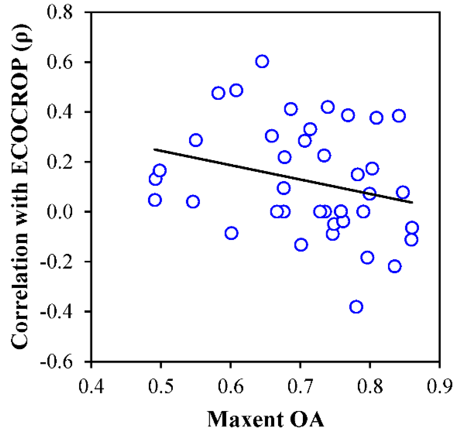
3.1. Model Accuracies

For the Maxent models, OA varied from 0.49 to 0.86 depending on the crop, with a mean value of 0.70 (Supplementary Table S5). AUC was highly similar to OA, with a range of 0.49–0.86 and a mean of 0.70. The Maxent accuracies were generally higher for annual crops than for permanent crops, and the accuracies generally increased with the areas covered by the crops. As such, the most common crops (potatoes, carrots, peas (Pisum sativum), apples (Malus domestica), and onions (Allium cepa var. cepa)) all had high predictive accuracies, while the least common crops (cucumbers (Cucumis sativus), tomatoes (Solanum lycopersicum), and elder (Sambucus nigra)) had low predictive accuracies.
ECOCROP generally did not accurately predict land use patterns. OA varied from 0.45 to 0.63 with a mean value of 0.50, and AUC varied from 0.36 to 0.76 with a mean value of 0.56 (Supplementary Table S6). As the holdout datasets for the accuracy assessments contained equal numbers of presence and absence points, an OA and AUC of 0.50 would be on par with a random guess. Furthermore, the accuracies for ECOCROP had a slight negative relationship with the Maxent accuracies for the same crops (r = −0.28).
Spearman rank correlation between the Maxent and ECOCROP suitabilities ranged from moderately negative (−0.38 for potatoes) to moderately positive (0.60 for gherkin (Cucumis sativus)) with a mean of 0.12 and standard deviation of 0.22 (Supplementary Table S7). Therefore, correlation between the Maxent and ECOCROP suitabilities was generally slightly positive, but only very generally, as the range of variation was very large. Furthermore, there was a slight negative relationship between OA for the Maxent models and their rank correlation with ECOCROP (r = −0.27) (Figure 3). Therefore, the most accurate Maxent models generally had the weakest correlation with the ECOCROP suitabilities.

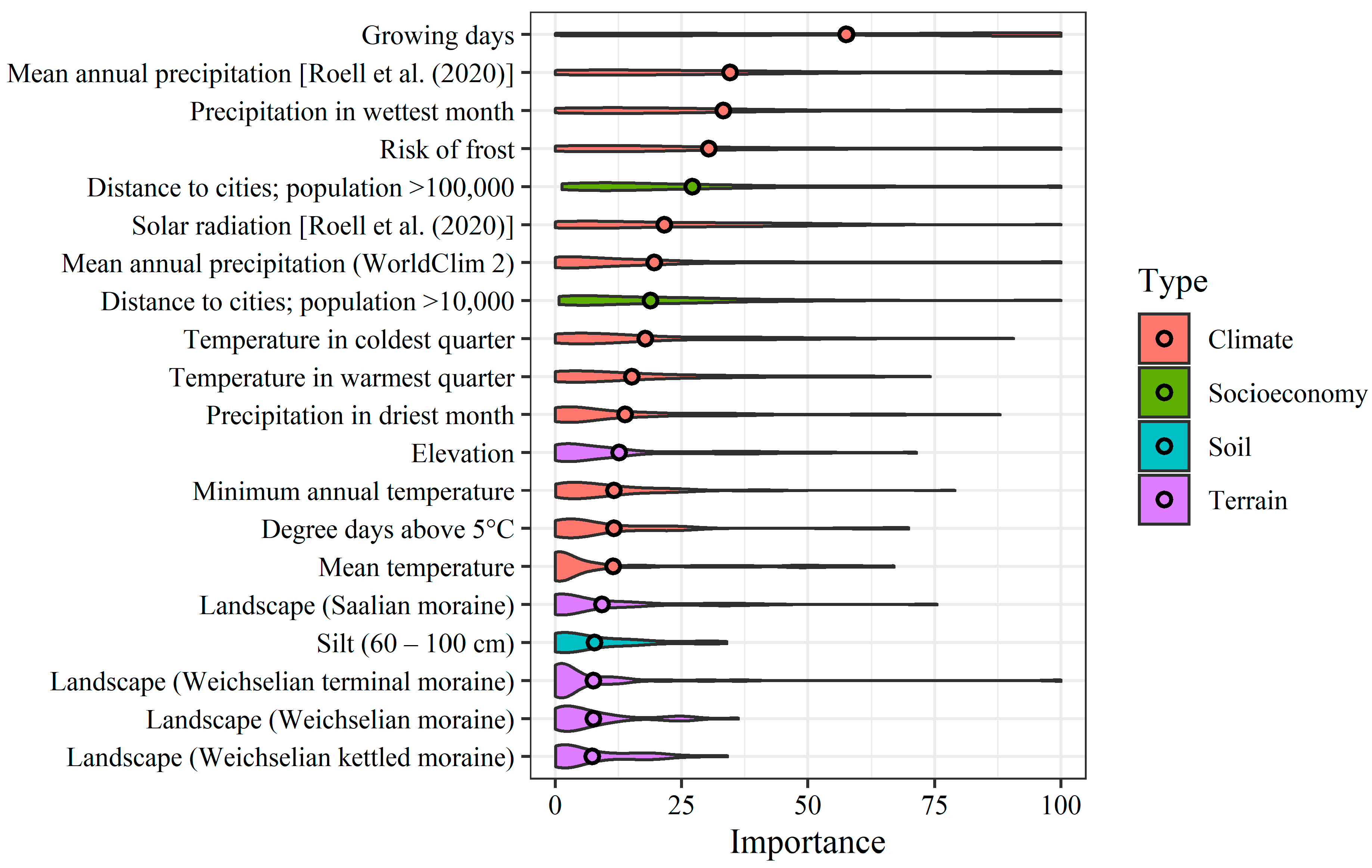
3.2. Covariate Importance

Climatic and socioeconomic covariates were the two most important categories in the Maxent models (Figure 4). In the extreme cases, climatic and socioeconomic covariates were several times more important than the topographic and soil-related covariates. The number of growing days and annual precipitation from [74] and precipitation in the wettest month from the WorldClim 2 dataset [73] were the three most important covariates. Furthermore, elevation was the most important terrain-related covariate with a mean importance of 13 (rank 12). The most important soil-related covariate was silt contents in the depth interval 60–100 cm, with a mean importance of 8 (rank 17).
The high importance of growing days and precipitation conforms to existing knowledge on the factors that affect crops in Denmark. For example, ref. [88] found that these two factors were highly important for predicting winter wheat yields in Denmark. However, it is surprising that climatic and socioeconomic covariates superseded nearly all terrain and soil-related covariates. The low importance of terrain-related covariates may be due to the relatively flat terrain in Denmark, which reduces effects from topography. However, previous studies have shown that soil properties have a strong effect on growing conditions in Denmark. Ref. [76] reported that differences in soil texture had large effects on rooting depth and plant-available water. Likewise, ref. [88] found that clay contents in the topsoil were the second most important covariate for predicting winter wheat yields. Furthermore, Denmark is a relatively small country, and many of the crops in this study have ranges far outside the boundaries of Denmark. Therefore, it is unlikely that climate explains as much of the variation in land use patterns inside Denmark as the covariate importance would indicate. Therefore, growing conditions cannot fully explain why climate-related covariates have a much higher importance than soil-related covariates in the Maxent models.

3.3. Examples

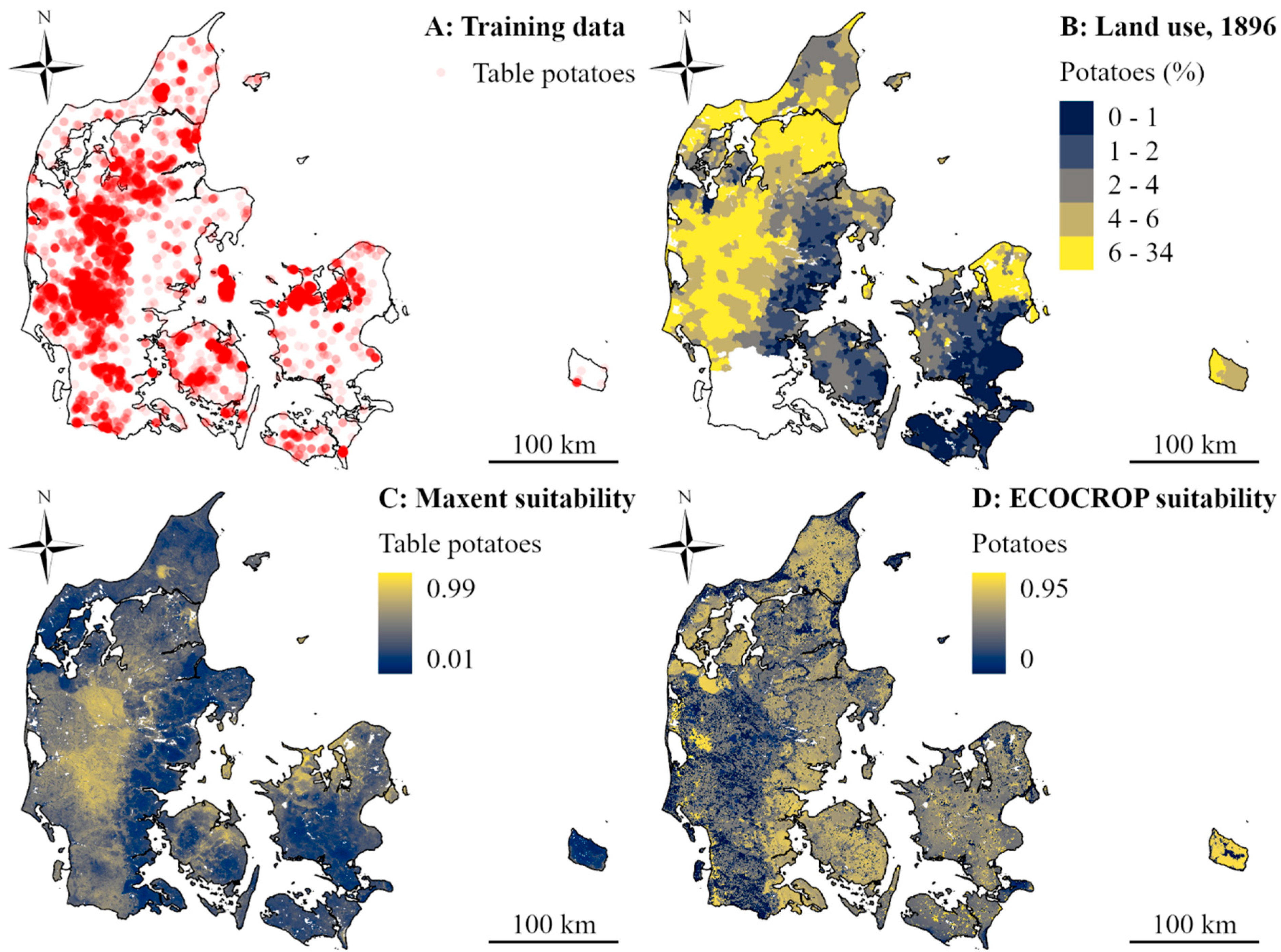
3.3.1. Table Potatoes
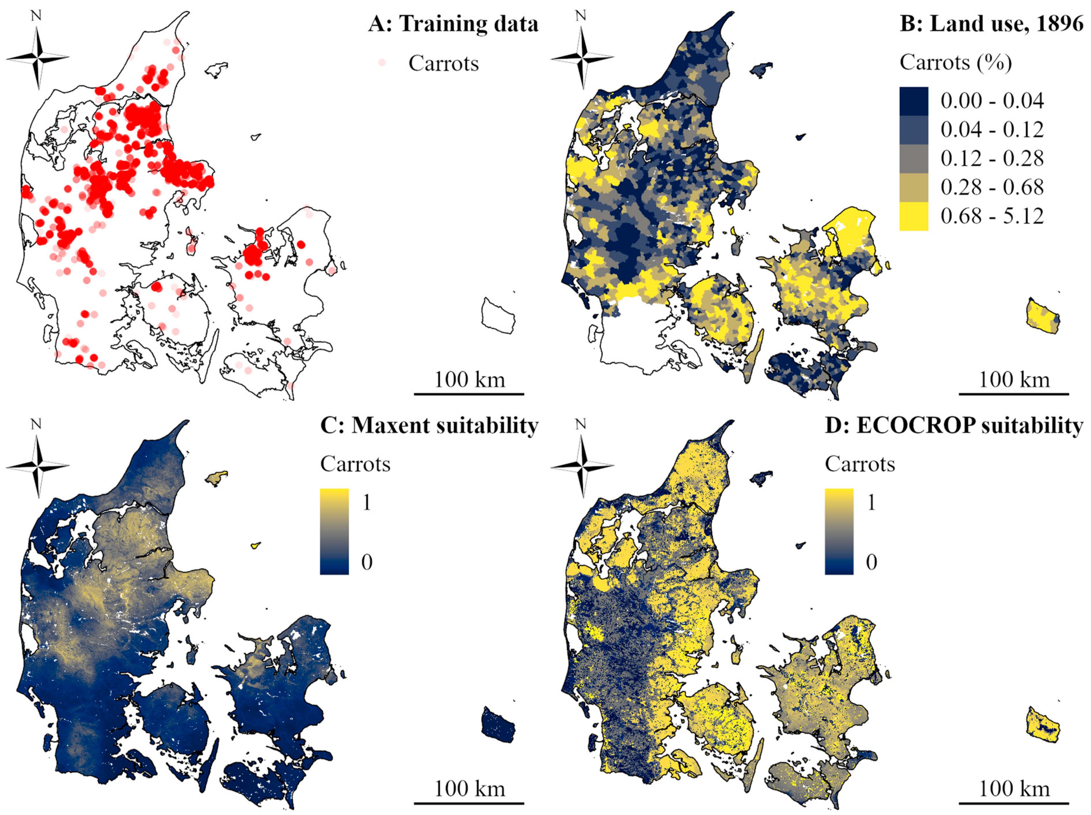
The Maxent model for table potatoes had a high OA (0.78) and AUC (0.78). Meanwhile, the ECOCROP suitabilities did not align with the presence or absence of potatoes, with an OA and AUC of 0.49, which is roughly on par with a random guess. Furthermore, the suitabilities predicted with Maxent had a negative rank correlation of −0.38 with the ECOCROP suitabilities.
The Maxent suitabilities followed the present land use, as the sandy glaciofluvial plains of western Denmark contained most of the highly suitable areas (Figure 5C). They also showed smaller areas with high suitability on organic soils in the northern part of the country. Suitabilities were generally low in the eastern part of the country, with an exception in a large reclaimed area in Zealand and a few other areas. Therefore, the parent materials in the areas with high suitabilities were highly variable, including glaciofluvial sand, loamy till, organic soils, and marine deposits. In addition, the soil texture and climate of these areas were also very different.
The ten most important covariates in the Maxent model included eight climatic covariates and two soil-related covariates (Table 2). The most important climatic covariates were solar radiation from [74], the risk of frost, and the mean annual precipitation. The two soil-related covariates were the post-glacial marine landscape type and silt contents in the depth interval 60–100 cm.
In contrast to the Maxent suitabilities, the most highly suitable areas according to ECOCROP were the loamy soils in the eastern part of the country (Figure 5D). According to the ECOCROP database, medium-textured soils are more suitable for potatoes than light-textured soils. Furthermore, the relatively dry climate and higher temperatures in the eastern part of the country should favor potatoes, according to the ECOCROP database. The only condition that favors potatoes in the western part of the country is the relatively low soil pH, as the ECOCROP database lists an optimal pH range of 5.0–6.2 for potatoes (Table 1). However, the soil pH maps had a scaled importance of <1 in the Maxent model and a rank of 54 or lower. Therefore, soil pH only had a minimal influence on the Maxent suitabilities.
The historic land use in 1896 was generally in agreement with the land use in the years 2011–2019, with a large presence of potatoes on the sandy soils of western Denmark. This shows that the general land use patterns for potatoes have remained mostly stable over time.

3.3.2. Carrots

The Maxent model for carrots had a high OA (0.84) and AUC (0.84). Meanwhile, the ECOCROP suitabilities did not accurately predict land use for carrots, with an OA of 0.50 and an AUC of 0.42. In addition, the Maxent suitabilities had a negative rank correlation with the ECOCROP suitabilities for carrots (−0.22).
The Maxent model mainly predicted a high suitability for carrots on sandy soils in the western and northern parts of the country (Figure 6). These soils, including mainly sandy till and glaciofluvial outwash plains, are generally well drained. There was also a small presence of highly suitable areas in and around the reclaimed area in the eastern part of the country, which also had a high Maxent suitability for potatoes.
For the Maxent model, eight of the ten most important covariates were climatic variables (Table 2). Furthermore, the distance to cities with populations >10,000 was the eighth most important covariate, and the phosphorus sorption capacity in the depth interval 25–50 cm was the 10th most important covariate. There were generally fewer carrot fields near cities, but it is not clear what caused this trend. At the same time, most carrot fields coincided with strongly leached sandy soils in western Denmark, which have a high phosphorus sorption capacity at 25–50 cm [71].
The ECOCROP suitabilities mostly contrasted with the Maxent suitabilities, as according to the ECOCROP database, light-textured soils are less suitable for carrots than medium-textured soils. Therefore, the sandy soils in western Denmark had low suitability for carrots according to ECOCROP. Warmer temperatures in eastern Denmark also contributed to this trend. Precipitation in some parts of Zealand was below the optimal range of 600–1200 mm listed in the ECOCROP database (Table 1). However, most of eastern Denmark was still highly suitable for carrots, according to ECOCROP.
The historic land use for the year 1896 agreed mostly with the ECOCROP suitability, as most of the parishes with a large presence of carrots were located in areas with loamy soils in eastern Denmark. In contrast, most of the areas with high Maxent suitability and a large presence of carrots in the years 2011–2019 had a low fraction of carrots in 1896. Therefore, the land use patterns for carrots have mostly reversed between 1896 and the years 2011–2019.

4. Discussion

4.1. Differences between Maxent and ECOCROP

The accuracies for Maxent were generally higher than the accuracies for ECOCROP. However, the accuracies mainly showed the ability of the models to predict the observed land use patterns. A fully accurate suitability map would simply replicate the land use and have no additional value relative to a land use map. Therefore, the higher accuracies of Maxent mainly show that they align more closely with the observed land use, but it does not necessarily show that they give a better indication of land suitability.
Furthermore, there was no general relationship between the Maxent and ECOCROP suitabilities. Correlation between the suitabilities were both positive and negative, and in most cases, correlation was close to zero. Moreover, the accuracies of the Maxent models give no indication of their correlation with the ECOCROP suitabilities. At the same time, neither Maxent nor ECOCROP suitabilities show any general relationship with historic land use data. For carrots, ECOCROP suitabilities agreed most closely with the historic land use data, but for potatoes, the Maxent suitabilities showed the highest agreement with the historic data.
It is possible that some of the discrepancies between the Maxent suitabilities, ECOCROP suitabilities, and the historic land use are due to errors in the models. For example, according to ECOCROP, the climate in Denmark should be fully unsuitable for apples, as the climatic suitability was 0 for the entire study area. However, there are about 1500 ha of apple orchards in Denmark, which makes apples one of the most common specialty crops in the country (Supplementary Table S1). Therefore, it is possible that the thresholds listed in the ECOCROP database are not appropriate for Denmark. Likewise, many of the fields with potatoes or carrots were located in areas that should be nearly or fully unsuitable for these crops, according to ECOCROP.
It is also possible that some of the discrepancies are due to low predictive accuracies in the Maxent models, as some of the models had very low accuracies. However, even when the models had high predictive accuracies, there was no general relationship with ECOCROP.
Furthermore, some of the discrepancies may have arisen from the way that we conceptualized this study. We tested the accuracies of the ECOCROP suitabilities using both presence and absence observations. However, the fact that an area fulfills the ecological requirements for one crop does not preclude the cultivation of other crops in the same area. For some crops, e.g., beets (Beta vulgaris var. conditiva), the ECOCROP suitabilities were high in most of the country. In these cases, the observed land use does not necessarily contradict ECOCROP, but neither does ECOCROP explain the observed land use patterns.
In this regard, it is also relevant that both soil pH and drainage, which we used in ECOCROP, are managed soil properties in Denmark [66,67]. Through liming, fertilization, and artificial drainage, farmers have changed the properties of Danish soils to improve their fertility. In this way, farmers have overcome limitations to cultivation in many areas of Denmark, and the soils therefore no longer reflect the natural environmental conditions. This reduces the usefulness of ECOCROP as a means for explaining observed land use patterns.

4.2. Effects of Socioeconomic Variables

While the points mentioned above may explain the lack of a relationship in individual cases, the complete lack of a general relationship is highly conspicuous. Notwithstanding the issues mentioned, it is clear that (1) ECOCROP does not account for specific land use patterns, and (2) Maxent suitabilities show no general relationship with the ecological crop requirements. The most likely reason for these two findings is that ECOCROP accounts only for environmental growing conditions, whereas ML can incorporate socioeconomic variables.
One previous study [48] found that socioeconomic variables were highly relevant for mapping land suitability, but only a small number of ML studies have employed them since then [50,80]. In this regard, it is important to emphasize that the widespread omission of socioeconomic variables in ML models for mapping land suitability does not mean that socioeconomic factors do not affect the resulting maps. Two studies [91,92] showed that ML models can successfully use inappropriate covariates for mapping spatial patterns, as long as the covariates contain spatial autocorrelation. In fact, ML models can predict spatial patterns from covariates that account only for spatial position [93,94,95]. In land suitability studies, this question has received relatively little attention, although [48] suggested that some variables might be proxies for unmeasured social phenomena.
In the present study, we used only two socioeconomic covariates, but we found that both of them had a high importance in the Maxent models. Furthermore, unaccounted-for socioeconomic variables may explain some of the many discrepancies between ECOCROP and Maxent. The importance of the climatic covariates was generally unexpectedly high in this study. A reason for this may be that the climatic variables to some extent act as proxies for socioeconomic trends with similar geographic range. Additionally, some environmental conditions, such as soil pH and drainage in Denmark, may reflect human actions and thereby socioeconomic trends.
Lastly, ECOCROP does not account for market prices and competition between crops, although they play a large role in shaping land use patterns. Therefore, a different approach is necessary in order to explain and predict land use patterns. [23] provided an example in a study comparing ML and socioeconomic land systems models for mapping land suitability in a 25,000-ha area in the Philippines. In this example, maize occupied flat areas, whereas bananas dominated steeper slopes. The authors argued that the higher economic returns from maize influenced this pattern, as both crops had good growing conditions in flat areas. Therefore, bananas occupied the slopes because slope gradient was a limiting factor for maize, not because the steep areas had optimal growing conditions for bananas. In the present study, a similar explanation may apply to the high Maxent suitabilities for table potatoes and carrots on the sandy soils in western Denmark. According to ECOCROP, both crops have optimal growing conditions in eastern Denmark, but farmers in eastern Denmark may prefer other crops with higher economic returns. For example, [88] showed that eastern Denmark had the highest yields for wheat, and the region also holds the highest concentration of wheat cultivation in Denmark [62]. In the less fertile areas of western Denmark, there is less competition from other crops and a higher presence of potatoes and carrots. Therefore, ML models may not explicitly account for competition between crops, but competition still affects land use patterns and thereby the land suitabilities predicted by the models.

4.3. Ecological and Socioeconomic Suitability

Based on these considerations, we suggest that researchers should apply different labels to the land suitabilities that they map, depending on the method. We suggest that suitability maps based on ECOCROP and other mechanistic models display ecological suitability, whereas suitability maps based on land systems models or ML models trained on land use data display socioeconomic suitability. While ecological suitability focuses on crop requirements, socioeconomic suitability is mainly concerned with the benefits for the farmer. Crop requirements still affect socioeconomic suitability, but the term also comprises socioeconomic factors and competition between crops. Conventional land evaluation can account for both forms of suitability, depending on the factors that researchers choose to include in the analysis.
Most previous studies have not made a clear distinction between ecological and socioeconomic suitability. This lack of clarity can potentially lead to misunderstandings, inappropriate choice of methods, and false conclusions. For example, the assumption that land use reflects ecological suitability may lead researchers to omit socioeconomic variables from the analysis. Then, the interpretation of the resulting model would give a false impression of the factors that affect the crop, their effects, and the areas where growing conditions are optimal. The consequences could include poor crop choices and agricultural management or inadequate policy decisions. It is always important to be cautious when interpreting ML models [91,92]. However, when it is unclear what the mapped variable represents, interpretation becomes even more hazardous, with a large risk of misinterpretation.
The risk of misinterpretation is especially relevant when researchers aim to map temporal shifts in land suitability. Studies aiming to map climate-induced changes in land suitability using ML have generally focused on growing conditions [41,42,43,44,45,46,52], implicitly aiming to map ecological suitability, omitting socioeconomic variables. Therefore, they could not identify important socioeconomic variables, their effects, and their interactions. This is problematic when aiming to map temporal trends, as socioeconomic variables are subject to changes over time. In fact, socioeconomic changes, such as technological developments and market dynamics can have larger effects than changes in environmental variables. For example, the acid soils of the Brazilian Cerrado biome were largely unsuitable for agriculture until technological developments including soil improvement and the development of new crop varieties made cultivation possible [96]. In the present study, the land use for carrots in Denmark showed a near reversal since 1896. This change is not due to changes in any environmental variable. On the contrary, agricultural developments, such as the increased use of fertilizer and irrigation, have enabled carrot cultivation on the previously infertile soils of western Denmark. Therefore, it is also highly likely that socioeconomic changes will strongly affect future land use. Moreover, future developments may also change interactions between the variables that decide socioeconomic suitability, which would invalidate the use of ML models.
Furthermore, while the land use patterns for carrots changed drastically over the course of the 20th century in Denmark, the land use patterns for potatoes were more stable. However, this stability does not mean that the land use reflected the ecological crop requirements. On the contrary, the land use for potatoes in both periods conflicted with the ecological crop requirements. This suggests that land use patterns are likely to reflect socioeconomic suitability, even when the land use is mostly stable.

4.4. Ways Forward for Future Studies

We acknowledge that our findings may not be fully representative and have some limitations. Firstly, the study area that we used was relatively small and strongly affected by human actions. In contrast, some studies using ML for land suitability assessment have worked at the global level [42,45]. With larger study areas, environmental variables, such as the climate, are more likely to affect land use patterns, and therefore, the relative effects of socioeconomic variables may be smaller. However, no studies have tested this assumption, so it should be a goal for future studies to address this question.
Secondly, some previous studies calibrated the thresholds found in the ECOCROP database [26,28]. We did not calibrate the thresholds in this study, which probably explains some of the observed discrepancies between the land use and the ECOCROP suitabilities. However, our results also indicate that researchers should be cautious when calibrating the thresholds found in the ECOCROP database, as the land use may reflect socioeconomic trends.
Thirdly, our validation datasets comprised only land use observations. Therefore, the predictive accuracies did not indicate the abilities of the models to assess the actual land suitability. However, this is a common shortcoming in land suitability assessment. Furthermore, a necessary step in resolving this issue is to define the type of the suitability that the map should reflect, as we pointed out in the previous section.
Methodological adaptations can alleviate some of the issues that we have raised. For example, the inclusion of socioeconomic variables in the analysis can enhance ML as a tool for explaining the observed land use. Alternatively, a smaller number of studies have used a subset of observations with high yields or produce quality for mapping land suitability [49,53,79]. One study [49] compared land suitability maps produced in this way with maps produced with all available land use observations as well as observed and modeled yields for maize (Zea mays) in South Africa. They found that the Maxent suitabilities based on the full dataset correlated poorly with observed and modeled yields, but models trained on the high-yielding subset correlated more closely with observed yields. Therefore, the selection of training locations based on yield or crop quality can increase the likelihood that the maps reflect ecological suitability.
However, the most urgent need in future studies is an increased awareness that land suitability can have different meanings depending on the context. Researchers should explicitly state whether they aim to map ecological or socioeconomic suitability, and they need to ensure that the methods are appropriate for the purpose. Preferably, researchers should conduct analyses to determine if it is possible to isolate ecological suitability from socioeconomic suitability and, if so, how. For example, researchers could compare ML suitabilities to land suitabilities based on crop requirements. If the ML suitabilities align with the ecological suitabilities, it is likely that ecological crop requirements are the main driver behind the land use. Otherwise, if the suitabilities deviate from each other, it is likely that socioeconomic variables have a strong influence on the land use. Furthermore, the analyses should include ML setups with and without socioeconomic variables, with a full set of locations and with a subset of locations. Finally, researchers should consider if ML is the best choice for their purposes.
It may also be necessary to elaborate on socioeconomic suitability as a term. As mentioned, conventional land suitability assessment focuses on the societal benefits from different land uses and in some cases environmental issues. However, the land suitability mapped with ML mainly reflects the choices of farmers. Societal and environmental considerations may affect cropping choices, for example through policies and regulations, but economic returns play a dominant role in shaping land use patterns at the farm level. Therefore, it is important to consider if land suitability should reflect societal, environmental, or farmers’ perspectives, or a compromise between these views. Moreover, researchers should determine how their methods could optimally reflect this choice.
In summary, ML does not obviate the need for expert evaluation in land suitability assessment. In fact, the need for expert knowledge may be greater than ever before.

5. Conclusions

In this study, we aimed to compare maps of land suitability produced by machine learning (ML) models trained on land use data with maps based on the mechanistic crop requirements model ECOCROP. The results showed that ML could often identify the areas where farmers typically grow specific crops. This was especially true for the most common specialty crops, such as potatoes, carrots, peas, apples, and onions. In two specific examples (potatoes and carrots), the predictive accuracies were high. However, the ML and ECOCROP suitabilities showed contrasting patterns. The ML suitabilities were highest on sandy soils in the western part of the country, where ECOCROP suitabilities were low. In fact, there was no general relationship between suitabilities predicted by ML and ECOCROP. In addition, ECOCROP suitabilities generally did not align with land use patterns.
Based on these discrepancies, we have argued that the meaning of the term land suitability is not sufficiently clear. We proposed instead that researchers should use the terms ecological suitability and socioeconomic suitability to avoid confusion and ensure that methods align with the purposes of the research. Furthermore, we argued that in most cases, ML models based on land use data predict mainly socioeconomic suitability. Even without the inclusion of socioeconomic variables, the patterns predicted by ML models are likely to reflect socioeconomic trends, as ML models can use other covariates as proxies.
Therefore, it is vital that researchers consider the purposes of their research and the form of suitability that they aim to map before they decide which methods to use. Specifically, if researchers aim to predict ecological suitability, they should use a subset of locations with high yields or produce quality. Alternatively, if the aim is to predict socioeconomic suitability, the analysis should also include socioeconomic variables.

Supplementary Materials

The following are available online at https://www.mdpi.com/article/10.3390/agronomy11040703/s1, Tables S1–S7. The tables list the crops investigated in the study (Table S1), the covariates used (Table S2), the climatic requirements for each crop according to ECOCROP (Table S3), the soil requirements for each crop according to ECOCROP (Table S4), the accuracies of the Maxent models (Table S5), the accuracies of ECOCROP (Table S6), and the rank correlations between the Maxent and ECOCROP suitabilities for each crop (Table S7).

Author Contributions

Conceptualization, A.B.M., V.L.M., G.B.M.H. and M.H.G.; methodology, A.B.M., V.L.M. and G.B.M.H.; software, A.B.M.; validation, A.B.M.; formal analysis, A.B.M.; investigation, A.B.M., V.L.M. and G.B.M.H.; resources, A.B.M., V.L.M. and M.H.G.; data curation, A.B.M. and N.M.J.; writing—original draft preparation, A.B.M.; writing—review and editing, A.B.M., V.L.M., G.B.M.H., N.M.J. and M.H.G.; visualization, A.B.M.; supervision, V.L.M., G.B.M.H. and M.H.G.; project administration, M.H.G.; funding acquisition, A.B.M., V.L.M. and M.H.G. All authors have read and agreed to the published version of the manuscript.

Funding

The Innovation Fund Denmark funded this research as part of the project ProvenanceDK (grant number 6150.00035B). The Agricultural School of Nordsjælland Foundation facilitated the research through a travel grant. V.L. Mulder is member of the research consortium GLADSOILMAP supported by LE STUDIUM Loire Valley Institute for Advanced Studies through its LE STUDIUM Research Consortium Program.

Institutional Review Board Statement

Not applicable.

Informed Consent Statement

Not applicable.

Data Availability Statement

The data presented in this study are available on request from the corresponding author. The data are not publicly available due to restrictions in data ownership.

Acknowledgments

The authors would like to thank Jetse Stoorvogel, who provided feedback and suggestions for the initial work on the manuscript.

Conflicts of Interest

The authors declare no conflict of interest.

References

  1. Mulder, V.L.; van Eck, C.M.; Friedlingstein, P.; Arrouays, D.; Regnier, P. Controlling factors for land productivity under extreme climatic events in continental Europe and the Mediterranean Basin. Catena 2019, 182, 104124. [Google Scholar] [CrossRef]
  2. Thompson, N.M.; Bir, C.; Widmar, N.J.O. Farmer perceptions of risk in 2017. Agribusiness 2018, 35, 182–199. [Google Scholar] [CrossRef]
  3. Duveiller, E.; Singh, R.P.; Nicol, J.M. The challenges of maintaining wheat productivity: Pests, diseases, and potential epidemics. Euphytica 2007, 157, 417–430. [Google Scholar] [CrossRef]
  4. O’Brien, K.; Leichenko, R.; Kelkar, U.; Venema, H.; Aandahl, G.; Tompkins, H.; Javed, A.; Bhadwal, S.; Barg, S.; Nygaard, L.; et al. Mapping vulnerability to multiple stressors: Climate change and globalization in India. Glob. Environ. Chang. 2004, 14, 303–313. [Google Scholar] [CrossRef]
  5. Lennox, E. Double Exposure to Climate Change and Globalization in a Peruvian Highland Community. Soc. Nat. Resour. 2015, 28, 781–796. [Google Scholar] [CrossRef]
  6. Cheshire, L.; Woods, M. Globally engaged farmers as transnational actors: Navigating the landscape of agri-food globalization. Geoforum 2013, 44, 232–242. [Google Scholar] [CrossRef]
  7. Brinkman, S.; Young, A. A Framework for Land Evaluation; Food and Agriculture Organisation of the United Nations: Wagening, The Netherlands, 1976; p. 89. [Google Scholar]
  8. Beek, K.J. Land Evaluation for Agricultural Development; ILRI: Wageningen, The Netherlands, 1978. [Google Scholar]
  9. Sonneveld, M.P.W.; Hack-ten Broeke, M.J.D.; van Diepen, C.A.; Boogaard, H.L. Thirty years of systematic land evaluation in the Netherlands. Geoderma 2010, 156, 84–92. [Google Scholar] [CrossRef]
  10. Rossiter, D.G. A theoretical framework for land evaluation. Geoderma 1996, 72, 165–190. [Google Scholar] [CrossRef]
  11. Geerts, S.; Raes, D.; Garcia, M.; Del Castillo, C.; Buytaert, W. Agro-climatic suitability mapping for crop production in the Bolivian Altiplano: A case study for quinoa. Agric. For. Meteorol. 2006, 139, 399–412. [Google Scholar] [CrossRef]
  12. Araya, A.; Keesstra, S.D.; Stroosnijder, L. A new agro-climatic classification for crop suitability zoning in northern semi-arid Ethiopia. Agric. For. Meteorol. 2010, 150, 1057–1064. [Google Scholar] [CrossRef]
  13. Boitt, M.K.; Mundia, C.N.; Pellikka, P.K.E. Land suitability assessment for effective crop production, a case study of Taita Hills, Kenya. J. Agric. Inform. 2015, 6. [Google Scholar] [CrossRef] [Green Version]
  14. El Baroudy, A.A. Mapping and evaluating land suitability using a GIS-based model. Catena 2016, 140, 96–104. [Google Scholar] [CrossRef]
  15. Purnamasari, R.A.; Ahamed, T.; Noguchi, R. Land suitability assessment for cassava production in Indonesia using GIS, remote sensing and multi-criteria analysis. Asia Pac. J. Reg. Sci. 2018, 3, 1–32. [Google Scholar] [CrossRef]
  16. Iliquín Trigoso, D.; Salas López, R.; Rojas Briceño, N.B.; Silva López, J.O.; Gómez Fernández, D.; Oliva, M.; Quiñones Huatangari, L.; Terrones Murga, R.E.; Barboza Castillo, E.; Barrena Gurbillón, M.Á. Land Suitability Analysis for Potato Crop in the Jucusbamba and Tincas Microwatersheds (Amazonas, NW Peru): AHP and RS–GIS Approach. Agronomy 2020, 10, 1898. [Google Scholar] [CrossRef]
  17. Brisson, N.; King, D.; Nicoullaud, B.; Ruget, F.; Ripoche, D.; Darthout, R. A crop model for land suitability evaluation a case study of the maize crop in France. Eur. J. Agron. 1992, 1, 163–175. [Google Scholar] [CrossRef]
  18. Katawatin, R.; Crown, P.H.; Grant, R.E. Simulation modelling of land suitability evaluation for dry season peanut cropping based on water availability in Northeast Thailand: Evaluation of the MACROS crop model. Soil Use Manag. 1996, 12, 25–32. [Google Scholar] [CrossRef]
  19. Littleboy, M.; Smith, D.M.; Bryant, M.J. Simulation modelling to determine suitability of agricultural land. Ecol. Model. 1996, 86, 219–225. [Google Scholar] [CrossRef]
  20. Schaldach, R.; Priess, J.A. Integrated Models of the Land System: A Review of Modelling Approaches on the Regional to Global Scale. Living Rev. Landsc. Res. 2008, 2. [Google Scholar] [CrossRef] [Green Version]
  21. Verburg, P.H.; Veldkamp, A. Projecting land use transitions at forest fringes in the Philippines at two spatial scales. Landsc. Ecol. 2004, 19, 77–98. [Google Scholar] [CrossRef]
  22. Luo, G.P.; Yin, C.Y.; Chen, X.; Xu, W.Q.; Lu, L. Combining system dynamic model and CLUE-S model to improve land use scenario analyses at regional scale: A case study of Sangong watershed in Xinjiang, China. Ecol. Complex. 2010, 7, 198–207. [Google Scholar] [CrossRef]
  23. Overmars, K.P.; Verburg, P.H.; Veldkamp, T.A. Comparison of a deductive and an inductive approach to specify land suitability in a spatially explicit land use model. Land Use Policy 2007, 24, 584–599. [Google Scholar] [CrossRef]
  24. Elnashar, A.; Abbas, M.; Sobhy, H.; Shahba, M. Crop Water Requirements and Suitability Assessment in Arid Environments: A New Approach. Agronomy 2021, 11, 260. [Google Scholar] [CrossRef]
  25. Manners, R.; Varela-Ortega, C.; van Etten, J. Protein-rich legume and pseudo-cereal crop suitability under present and future European climates. Eur. J. Agron. 2020, 113. [Google Scholar] [CrossRef]
  26. Ramirez-Villegas, J.; Jarvis, A.; Läderach, P. Empirical approaches for assessing impacts of climate change on agriculture: The EcoCrop model and a case study with grain sorghum. Agric. For. Meteorol. 2013, 170, 67–78. [Google Scholar] [CrossRef]
  27. Egbebiyi, T.S.; Crespo, O.; Lennard, C. Defining Crop–climate Departure in West Africa: Improved Understanding of the Timing of Future Changes in Crop Suitability. Climate 2019, 7, 101. [Google Scholar] [CrossRef] [Green Version]
  28. Piikki, K.; Winowiecki, L.; Vågen, T.-G.; Ramirez-Villegas, J.; Söderström, M. Improvement of spatial modelling of crop suitability using a new digital soil map of Tanzania. S. Afr. J. Plant Soil 2017, 34, 243–254. [Google Scholar] [CrossRef]
  29. Alemayehu, S.; Ayana, E.K.; Dile, Y.T.; Demissie, T.; Yimam, Y.; Girvetz, E.; Aynekulu, E.; Solomon, D.; Worqlul, A.W. Evaluating Land Suitability and Potential Climate Change Impacts on Alfalfa (Medicago sativa) Production in Ethiopia. Atmosphere 2020, 11, 1124. [Google Scholar] [CrossRef]
  30. Suhairi, T.A.S.T.M.; Jahanshiri, E.; Nizar, N.M.M. Multicriteria land suitability assessment for growing underutilised crop, bambara groundnut in Peninsular Malaysia. IOP Conf. Ser. Earth Environ. Sci. 2018, 169. [Google Scholar] [CrossRef]
  31. Remesh, K.R.R.; Byju, G.; Soman, S.; Raju, S.; Ravi, V. Future changes in mean temperature and total precipitation and climate suitability of yam (Dioscorea spp.) in major yam-growing environments in India. Curr. Hortic. 2019, 7. [Google Scholar] [CrossRef]
  32. Hunter, R.; Crespo, O. Large Scale Crop Suitability Assessment Under Future Climate Using the Ecocrop Model: The Case of Six Provinces in Angola’s Planalto Region. In The Climate-Smart Agriculture Papers: Investigating the Business of a Productive, Resilient and Low Emission Future; Rosenstock, T.S., Nowak, A., Girvetz, E., Eds.; Springer International Publishing: Cham, Switzerland, 2019; pp. 39–48. [Google Scholar]
  33. FAO. Crop Ecological Requirements Database (ECOCROP). Available online: http://www.fao.org/land-water/land/land-governance/land-resources-planning-toolbox/category/details/en/c/1027491/ (accessed on 21 October 2020).
  34. Samuel, A.L. Some Studies in Machine Learning Using the Game of Checkers. IBM J. Res. Dev. 1959, 3, 210–229. [Google Scholar] [CrossRef]
  35. McBratney, A.B.; Mendonça Santos, M.L.; Minasny, B. On digital soil mapping. Geoderma 2003, 117, 3–52. [Google Scholar] [CrossRef]
  36. Minasny, B.; McBratney, A.B. Digital soil mapping: A brief history and some lessons. Geoderma 2016, 264, 301–311. [Google Scholar] [CrossRef]
  37. Franklin, J. Mapping Species Distributions: Spatial Inference and Prediction; Cambridge University Press: Cambridge, UK, 2010. [Google Scholar]
  38. Martínez-Minaya, J.; Cameletti, M.; Conesa, D.; Pennino, M.G. Species distribution modeling: A statistical review with focus in spatio-temporal issues. Stoch. Environ. Res. Risk Assess. 2018, 32, 3227–3244. [Google Scholar] [CrossRef]
  39. Maxwell, A.E.; Warner, T.A.; Fang, F. Implementation of machine-learning classification in remote sensing: An applied review. Int. J. Remote Sens. 2018, 39, 2784–2817. [Google Scholar] [CrossRef] [Green Version]
  40. Maguranyanga, C.; Murwira, A. Mapping maize, tobacco, and soybean fields in large-scale commercial farms of Zimbabwe based on multitemporal NDVI images in MAXENT. Can. J. Remote Sens. 2015, 40, 396–405. [Google Scholar] [CrossRef]
  41. Kogo, B.K.; Kumar, L.; Koech, R.; Kariyawasam, C.S. Modelling Climate Suitability for Rainfed Maize Cultivation in Kenya Using a Maximum Entropy (MaxENT) Approach. Agronomy 2019, 9, 727. [Google Scholar] [CrossRef] [Green Version]
  42. Feng, L.; Wang, H.; Ma, X.; Peng, H.; Shan, J. Modeling the current land suitability and future dynamics of global soybean cultivation under climate change scenarios. Field Crop. Res. 2021, 263. [Google Scholar] [CrossRef]
  43. Chhogyel, N.; Kumar, L.; Bajgai, Y.; Sadeeka Jayasinghe, L. Prediction of Bhutan’s ecological distribution of rice (Oryza sativa L.) under the impact of climate change through maximum entropy modelling. J. Agric. Sci. 2020, 158, 25–37. [Google Scholar] [CrossRef]
  44. Läderach, P.; Martinez-Valle, A.; Schroth, G.; Castro, N. Predicting the future climatic suitability for cocoa farming of the world’s leading producer countries, Ghana and Côte d’Ivoire. Clim. Chang. 2013, 119, 841–854. [Google Scholar] [CrossRef] [Green Version]
  45. Ovalle-Rivera, O.; Laderach, P.; Bunn, C.; Obersteiner, M.; Schroth, G. Projected shifts in Coffea arabica suitability among major global producing regions due to climate change. PLoS ONE 2015, 10, e0124155. [Google Scholar] [CrossRef] [Green Version]
  46. Schroth, G.; Laderach, P.; Dempewolf, J.; Philpott, S.; Haggar, J.; Eakin, H.; Castillejos, T.; Garcia Moreno, J.; Soto Pinto, L.; Hernandez, R.; et al. Towards a climate change adaptation strategy for coffee communities and ecosystems in the Sierra Madre de Chiapas, Mexico. Mitig. Adapt. Strateg. Glob. Chang. 2009, 14, 605–625. [Google Scholar] [CrossRef] [Green Version]
  47. Heumann, B.W.; Walsh, S.J.; McDaniel, P.M. Assessing the application of a geographic presence-only model for land suitability mapping. Ecol. Inf. 2011, 6, 257–269. [Google Scholar] [CrossRef] [Green Version]
  48. Heumann, B.W.; Walsh, S.J.; Verdery, A.M.; McDaniel, P.M.; Rindfuss, R.R. Land Suitability Modeling using a Geographic Socio-Environmental Niche-Based Approach: A Case Study from Northeastern Thailand. Ann. Assoc. Am. Geogr. 2013, 103. [Google Scholar] [CrossRef] [PubMed]
  49. Estes, L.D.; Bradley, B.A.; Beukes, H.; Hole, D.G.; Lau, M.; Oppenheimer, M.G.; Schulze, R.; Tadross, M.A.; Turner, W.R. Comparing mechanistic and empirical model projections of crop suitability and productivity: Implications for ecological forecasting. Glob. Ecol. Biogeogr. 2013, 22, 1007–1018. [Google Scholar] [CrossRef]
  50. Akpoti, K.; Kabo-bah, A.T.; Dossou-Yovo, E.R.; Groen, T.A.; Zwart, S.J. Mapping suitability for rice production in inland valley landscapes in Benin and Togo using environmental niche modeling. Sci. Total Environ. 2020, 709, 136165. [Google Scholar] [CrossRef]
  51. Rodcha, R.; Tripathi, N.; Prasad Shrestha, R. Comparison of Cash Crop Suitability Assessment Using Parametric, AHP, and FAHP Methods. Land 2019, 8, 79. [Google Scholar] [CrossRef] [Green Version]
  52. Ranjitkar, S.; Sujakhu, N.M.; Merz, J.; Kindt, R.; Xu, J.; Matin, M.A.; Ali, M.; Zomer, R.J. Suitability Analysis and Projected Climate Change Impact on Banana and Coffee Production Zones in Nepal. PLoS ONE 2016, 11, e0163916. [Google Scholar] [CrossRef] [PubMed] [Green Version]
  53. Yang, M.; Li, Z.; Liu, L.; Bo, A.; Zhang, C.; Li, M. Ecological niche modeling of Astragalus membranaceus var. mongholicus medicinal plants in Inner Mongolia, China. Sci. Rep. 2020, 10, 12482. [Google Scholar] [CrossRef]
  54. White, R.E.; Balachandra, L.; Edis, R.; Chen, D. The soil component of terroir. OENO One 2007, 41, 9. [Google Scholar] [CrossRef] [Green Version]
  55. Costantini, E.A.C.; Bucelli, P. Soil and terroir. In Soil Security for Ecosystem Management; Kapur, S., Erşahin, S., Eds.; Springer: Berlin, Germany, 2014; pp. 97–133. [Google Scholar]
  56. Kærgård, N.; Dalgaard, T. Dansk landbrugs strukturudvikling siden 2. verdenskrig. Landbohistorisk Tidsskr. 2014, 11, 9–33. [Google Scholar]
  57. Statistics Denmark. Statistisk Årbog; Statistics Denmark: Copenhagen, Denmark, 2017.
  58. Wang, P.R. Referenceværdier: Døgn-, Måneds- og Årsværdier for Regioner og Hele Landet 2001–2010, Danmark for Temperatur, Relativ Luftfugtighed, Vindhastighed, Globalstråling og Nedbør; Teknisk Rapport 12-24; Danish Meteorological Institute: Copenhagen, Denmark, 2013.
  59. Adhikari, K.; Minasny, B.; Greve, M.B.; Greve, M.H. Constructing a soil class map of Denmark based on the FAO legend using digital techniques. Geoderma 2014, 214–215, 101–113. [Google Scholar] [CrossRef] [Green Version]
  60. Madsen, H.B.; Jensen, N.H. Soil map of Denmark according to the revised FAO legend 1990. Dan. J. Geogr. 1996, 96, 51–59. [Google Scholar] [CrossRef]
  61. Møller, A.B.; Malone, B.; Odgers, N.P.; Beucher, A.; Iversen, B.V.; Greve, M.H.; Minasny, B. Improved disaggregation of conventional soil maps. Geoderma 2019, 341, 148–160. [Google Scholar] [CrossRef]
  62. The Danish Agricultural Agency Kort og Markblokke. Available online: https://lbst.dk/landbrug/kort-og-markblokke/ (accessed on 14 October 2020).
  63. Agricultural Marketing Service. Definition of Specialty Crops; US Department of Agriculture: Washington, DC, USA, 2014.
  64. Adhikari, K.; Hartemink, A.E.; Minasny, B.; Kheir, R.B.; Greve, M.B.; Greve, M.H. Digital mapping of soil organic carbon contents and stocks in Denmark. PLoS ONE 2014, 9, e105519. [Google Scholar] [CrossRef]
  65. Adhikari, K.; Kheir, R.B.; Greve, M.B.; Bøcher, P.K.; Malone, B.P.; Minasny, B.; McBratney, A.B.; Greve, M.H. High-resolution 3-D mapping of soil texture in Denmark. Soil Sci. Soc. Am. J. 2013, 77, 860–876. [Google Scholar] [CrossRef]
  66. Adhikari, K.; Kheir, R.B.; Greve, M.B.; Greve, M.H.; Malone, M.; Minasny, B.; McBratney, A. Mapping soil pH and bulk density at multiple soil depths in Denmark. In GlobalSoilMap: Basis of the Global Spatial Soil Information System; Arrouays, D., McKenzie, N.J., Hempel, J., de Forges, A.R., McBratney, A., Eds.; Taylor & Francis: London, UK, 2014; pp. 155–160. [Google Scholar]
  67. Møller, A.B.; Beucher, A.; Iversen, B.V.; Greve, M.H. Predicting artificially drained areas by means of a selective model ensemble. Geoderma 2018, 320, 30–42. [Google Scholar] [CrossRef]
  68. Møller, A.B.; Beucher, A.; Iversen, B.V.; Greve, M.H. Prediction of soil drainage classes in Denmark by means of decision tree classification. Geoderma 2017, 352, 314–329. [Google Scholar] [CrossRef]
  69. Elith, J.; Phillips, S.J.; Hastie, T.; Dudík, M.; Chee, Y.E.; Yates, C.J. A statistical explanation of MaxEnt for ecologists. Divers. Distrib. 2011, 17, 43–57. [Google Scholar] [CrossRef]
  70. Yackulic, C.B.; Chandler, R.; Zipkin, E.F.; Royle, J.A.; Nichols, J.D.; Campbell Grant, E.H.; Veran, S.; O’Hara, R.B. Presence-only modelling using MAXENT: When can we trust the inferences? Methods Ecol. Evol. 2013, 4, 236–243. [Google Scholar] [CrossRef]
  71. Møller, A.B.; Heckrath, G.; Hermansen, C.; Nørgaard, T.; de Jonge, L.W.; Greve, M.H. Mapping the phosphorus sorption capacity of Danish soils with quantile regression forests and uncertainty propagation. 2021. in writing. [Google Scholar]
  72. Jakobsen, P.R.; Hermansen, B.; Tougaard, L. Danmarks Digitale Jordartskort 1:25,000 Version 4.0; 30; GEUS: Copenhagen, Denmark, 2015; p. 29. [Google Scholar]
  73. Fick, S.E.; Hijmans, R.J. WorldClim 2: New 1-km spatial resolution climate surfaces for global land areas. Int. J. Climatol. 2017, 37, 4302–4315. [Google Scholar] [CrossRef]
  74. Roell, Y.E.; Peng, Y.; Beucher, A.; Greve, M.B.; Greve, M.H. Development of hierarchical terron workflow based on gridded data—A case study in Denmark. Comput. Geosci. 2020, 138. [Google Scholar] [CrossRef]
  75. National Survey and Cadastre. Danmarks Højdemodel 2007, DHM-2007/Terræn; National Survey and Cadastre: Copenhagen, Denmark, 2012. [Google Scholar]
  76. Madsen, H.B.; Nørr, A.H.; Holst, K.A. The Danish Soil Classification; The Royal Danish Geographical Society: Copenhagen, Denmark, 1992; Volume 3, p. 56. [Google Scholar]
  77. Agency for Data Supply and Efficiency GeoDanmark. Available online: https://sdfe.dk/hent-data/fotos-og-geodanmark-data/ (accessed on 26 August 2020).
  78. Akpoti, K.; Kabo-bah, A.T.; Zwart, S.J. Agricultural land suitability analysis: State-of-the-art and outlooks for integration of climate change analysis. Agric. Syst. 2019, 173, 172–208. [Google Scholar] [CrossRef]
  79. López-Rocha, E.; Mireles-Arriga, A.I.; Hernández-Ruíz, J.; Ruiz-Nieto, J.E.; Rucoba-Garcia, A. Áreas potenciales para el cultivo de girasol en condiciones de temporal en Guanajuato, México. Agron. Mesoam. 2018, 29, 305. [Google Scholar] [CrossRef] [Green Version]
  80. Mbugua, J.K.; Suksa-ngiam, W. Predicting suitable areas for growing cassava using remote sensing and machine learning techniques: A study in Nakhon-Phanom Thailand. Issues Inf. Sci. Inf. Technol. 2018, 15, 43–56. [Google Scholar] [CrossRef] [Green Version]
  81. Phillips, S.J.; Dudík, M. Modeling of species distributions with Maxent: New extensions and a comprehensive evaluation. Ecography 2008, 31, 161–175. [Google Scholar] [CrossRef]
  82. Merow, C.; Smith, M.J.; Silander, J.A. A practical guide to MaxEnt for modeling species’ distributions: What it does, and why inputs and settings matter. Ecography 2013, 36, 1058–1069. [Google Scholar] [CrossRef]
  83. Phillips, S.J.; Dudík, M.; Schapire, R.E. Maxent Software for Modeling Species Niches and Distributions (Version 3.4.1). Available online: http://biodiversityinformatics.amnh.org/open_source/maxent/ (accessed on 31 March 2020).
  84. Hijmans, R.J.; Phillips, S.J.; Leathwick, J.; Elith, J. Package ‘dismo’: Species Distribution Modeling. Available online: https://cran.r-project.org/web/packages/dismo/dismo.pdf (accessed on 21 October 2020).
  85. Meyer, H.; Reudenbach, C.; Hengl, T.; Katurji, M.; Nauss, T. Improving performance of spatio-temporal machine learning models using forward feature selection and target-oriented validation. Environ. Model. Softw. 2018, 101, 1–9. [Google Scholar] [CrossRef]
  86. Brenning, A. Spatial cross-validation and bootstrap for the assessment of prediction rules in remote sensing: The R package sperrorest. Int. Geosci. Remote Sens. 2012, 5372–5375. [Google Scholar] [CrossRef]
  87. Robin, X.; Turck, N.; Hainard, A.; Tiberti, N.; Lisacek, F.; Sanchez, J.-C.; Müller, M.; Siegert, S.; Doering, M.; Robin, M.X. Package ‘pROC’. Available online: https://cran.r-project.org/web/packages/pROC/pROC.pdf (accessed on 26 January 2020).
  88. Roell, Y.E.; Beucher, A.; Møller, P.G.; Greve, M.B.; Greve, M.H. Comparing a Random Forest based prediction of winter wheat yield to historical yield potential. Agronomy 2020, 10, 395. [Google Scholar] [CrossRef] [Green Version]
  89. Bianco Lunos Hof-Trykkeri (F. Dreyer). Arealets Benyttelse i Danmark den 15. Juli 1896 (Statistisk Tabelværk Rk. 5 Litra C Nr 1); Statistics Denmark: Copenhagen, Denmark, 1898.
  90. DigDag Digital Atlas of Denmark’s Historical-Administrative Geography. Available online: http://digdag.dk (accessed on 26 January 2020).
  91. Fourcade, Y.; Besnard, A.G.; Secondi, J. Paintings predict the distribution of species, or the challenge of selecting environmental predictors and evaluation statistics. Glob. Ecol. Biogeogr. 2018, 27, 245–256. [Google Scholar] [CrossRef]
  92. Wadoux, A.M.J.C.; Samuel-Rosa, A.; Poggio, L.; Mulder, V.L. A note on knowledge discovery and machine learning in digital soil mapping. Eur. J. Soil Sci. 2019. [Google Scholar] [CrossRef]
  93. Hengl, T.; Nussbaum, M.; Wright, M.N.; Heuvelink, G.B.; Gräler, B. Random forest as a generic framework for predictive modeling of spatial and spatio-temporal variables. PeerJ 2018, 6, e5518. [Google Scholar] [CrossRef] [Green Version]
  94. Behrens, T.; Schmidt, K.; Viscarra Rossel, R.; Gries, P.; Scholten, T.; MacMillan, R. Spatial modelling with Euclidean distance fields and machine learning. Eur. J. Soil Sci. 2018, 69, 757–770. [Google Scholar] [CrossRef]
  95. Møller, A.B.; Beucher, A.M.; Pouladi, N.; Greve, M.H. Oblique geographic coordinates as covariates for digital soil mapping. Soil 2020, 6, 269–289. [Google Scholar] [CrossRef]
  96. Pereira, P.A.A.; Martha, G.B.; Santana, C.A.M.; Alves, E. The development of Brazilian agriculture: Future technological challenges and opportunities. Agric. Food Secur. 2012, 1. [Google Scholar] [CrossRef] [Green Version]
Figure 1. Block diagram showing an overview of the methods and data applied in the study.
Agronomy 11 00703 g001
Figure 2. Areas in Denmark with farmers’ registrations for the Common Agricultural Policy of the European Union in the years 2011–2019. The inset shows the location of Denmark in northern Europe.
Agronomy 11 00703 g002
Figure 3. Scatter plot of the overall accuracy (OA) of Maxent models for predicting land suitability for specialty crops and their rank correlation with the suitability for the same crops mapped with ECOCROP (Spearman’s rank correlation). The line shows the linear least squares regression between the two variables.
Agronomy 11 00703 g003
Figure 4. Violin plot showing the distributions of the importance of the 20 most important covariates in the Maxent models for predicting land suitability for specialty crops, scaled to 100 for the most important covariate in each model. Dots show the mean importance of each covariate across all models.
Agronomy 11 00703 g004
Figure 5. Land use and land suitability for table potatoes. (A) Training data for Maxent models to predict land suitability, extracted from fields with table potatoes in the years 2011–2019. Points have 90% transparency. (B) Fields with potatoes in 1896 as fraction of agricultural land at parish level. (C) Land suitability for table potatoes predicted by Maxent model trained from land use observations. (D) Land suitability for potatoes mapped based on values from the ECOCROP database. Suitabilities of 0 represent fully unsuitable land, while suitabilities of 1 represent optimally suited land.
Agronomy 11 00703 g005
Figure 6. Land use and land suitability for carrots. (A) Training data for Maxent models to predict land suitability for carrots, extracted from fields with carrots in the years 2011–2019. Points have 90% transparency. (B) Fields with carrots in 1896 as fraction of agricultural land at parish level. (C) Land suitability for carrots predicted by a Maxent model trained from land use observations. (D) Land suitability for carrots mapped based on values from the ECOCROP database. Suitabilities of 0 represent fully unsuitable land, while suitabilities of 1 represent optimally suited land.
Agronomy 11 00703 g006
Table 1. Minimum and maximum values for optimal and suitable growing conditions for potatoes and carrots, according to the ECOCROP (Ecological Crop Requirements) database. For soil texture and drainage, the table indicates the suitability value (0 = unsuitable; 1 = optimal) associated with each class.
CropPotatoCarrot
Growing season (days)
Minimum9040
Maximum160150
Temperature (°C)
Killing−1−1
Minimum, range73
Minimum, optimal1515
Maximum, optimal2524
Maximum, range3030
Precipitation (mm)
Minimum, range250400
Minimum, optimal500600
Maximum, optimal8001200
Maximum, range20004000
Soil texture
Light0.50.5
Medium11
Heavy0.50.5
Organic11
Soil drainage
Insufficient drainage00
Well-drained11
Soil pH
Minimum, range4.24.2
Minimum, optimal5.05.8
Maximum, optimal6.26.8
Maximum, range8.58.7
Table 2. Ten most important covariates in the Maxent models for mapping land suitability for table potatoes and carrots based on land use data.
RankTable PotatoesCarrots
1Solar radiation aGrowing days a
2Risk of frost aRisk of frost a
3Mean annual precipitation bPrecipitation in wettest month b
4Mean annual precipitation aDegree days above 5 °C
5Temperature in coldest quarter bPrecipitation in driest month b
6Landscape (post-glacial marine)Solar radiation a
7Precipitation in wettest month bMean annual precipitation a
8Minimum annual temperature bDistance to cities; population >10,000
9Precipitation in driest month bMinimum annual temperature b
10Silt (60–100 cm)Phosphorus sorption capacity (25–50 cm)
a From Roell et al. (2020); b From the BioClim 2 dataset.
Publisher’s Note: MDPI stays neutral with regard to jurisdictional claims in published maps and institutional affiliations.

