Assessing the Sentinel-2 Capabilities to Identify Abandoned Crops Using Deep Learning

Abstract

The termination or interruption of agro-forestry practices for a long period gradually results in abandoned land. Abandoned land parcels do not match the requirements to access to the basic payment of the European Common Agricultural Policy (CAP). Therefore, the identification of those parcels is key in order to return fair subsidies to farmers. In this context, the present work proposes a methodology to detect abandoned crops in the Valencian Community (Spain) from remote sensing data. The approach is based on the assessment of multitemporal Sentinel-2 images and derived spectral indices, which are used as predictors for training machine learning and deep learning classifiers. Several classification scenarios, including both abandoned and active parcels, were evaluated. The best results ($98.2\%$ overall accuracy) were obtained when a bi-directional Long Short Term Memory (BiLSTM) network was trained with a multitemporal dataset composed of twelve reflectance time series, and a derived bare soil spectral index (BSI). In this scenario we were able to effectively distinguish abandoned crops from active ones. The results revealed Sentinel-2 features are well suited for land use identification including abandoned lands, and open the possibility of implementing this type of remote sensing based methodology into the CAP payments supervision.

1. Introduction

The Common Agricultural Policy (CAP) is one of the most important European Commissions (EC) initiatives. It was created in 1962 with the objective of ensuring affordable and quality food across Europe, while supporting European farmers. With this aim, a system of agricultural subsidies was implemented. Within the European Green Deal (EGD) [1], policies were implemented to ensure a transition towards a more sustainable agriculture. From 2021 to 2027, there is a total budget of 365 billion Euros assigned for the CAP, which represents 28.5% of the overall EU budget for this period. About 265 billion Euros is used for direct payments to the farmers. The process for accessing subsidies requires declarations from the farmers indicating the extension of their parcels, and which type of agricultural activity is performed. If those activities do not fit the CAP requirements, payments could be cancelled. Every European member state (MS) has to supervise the declarations, which is carried out by state paying agencies. These agencies are responsible for supervising the declarations, a process that is typically done by in-situ checks or photo interpretation of high resolution images taken from airborne or satellite platforms. However, these methods are time consuming, require expert knowledge, and are unsuitable to be done over big areas. For this reason, the 2018 CAP regulation [2] proposed the use of data coming from Earth Observation (EO), in particular from the Copernicus program, to supervise the CAP 2020+ farmers declarations. The goal is to apply automated supervision for the majority of cases, based on Sentinel-1 and Sentinel-2 data, and leave cases (ideally up to 5% of the territory) that cannot be supervised by this procedure to the other methods (e.g., in situ checks and photo interpretation). Another strength of this approach could be the regular updating of state Land Parcel Identification Systems (LPIS), which allows paying agencies to uniquely identify land parcels in space, have a record of the given land use (and its evolution), and ultimately ease the declaration procedure to both farmers and paying agencies. CAP requirements are subject to the land cover extension, land cover use, and also to an optimum state of the parcel. This means that parcels without proper conditions for agricultural activities, or even abandoned parcels, do not match CAP requirements to access subsidies.

Crop type identification from EO is a widely covered topic that uses remote sensing data, with multiple works over the years, and some recent publications related to CAP subsidies monitoring [3,4,5]. However, cropland abandonment identification still presents some challenges from a remote sensing perspective, as it is a complex phenomenon with some different causes and possible outcomes [6]. The first attempts for crop type identification and abandonment detection relied on hand-crafted features based on spatial and temporal dynamics of vegetation [7,8]. However, machine learning and deep learning methods have become state of the art for this task. While the first require feeding the algorithms with meaningful features, deep learning architectures excel in extracting these features encoded in the data [9], and usually achieve very high accuracies in crop identification tasks [10,11], and also in abandonment detection [12]. Despite their excellent results, the majority of deep learning models are considered as “black-boxes”, whereby another relevant trend is seeking interpretability of these algorithms, for improved decision making [13].

In this context, this paper aims to assess the potential of Sentinel-2 time series for land abandonment detection in the Valencia province in Spain. The approach is based on the evaluation of Sentinel-2 derived spectral indices’ time series, and on the assessment of the classification power of different machine learning and deep learning algorithms for discriminating abandoned parcels.

2. Materials and Methods

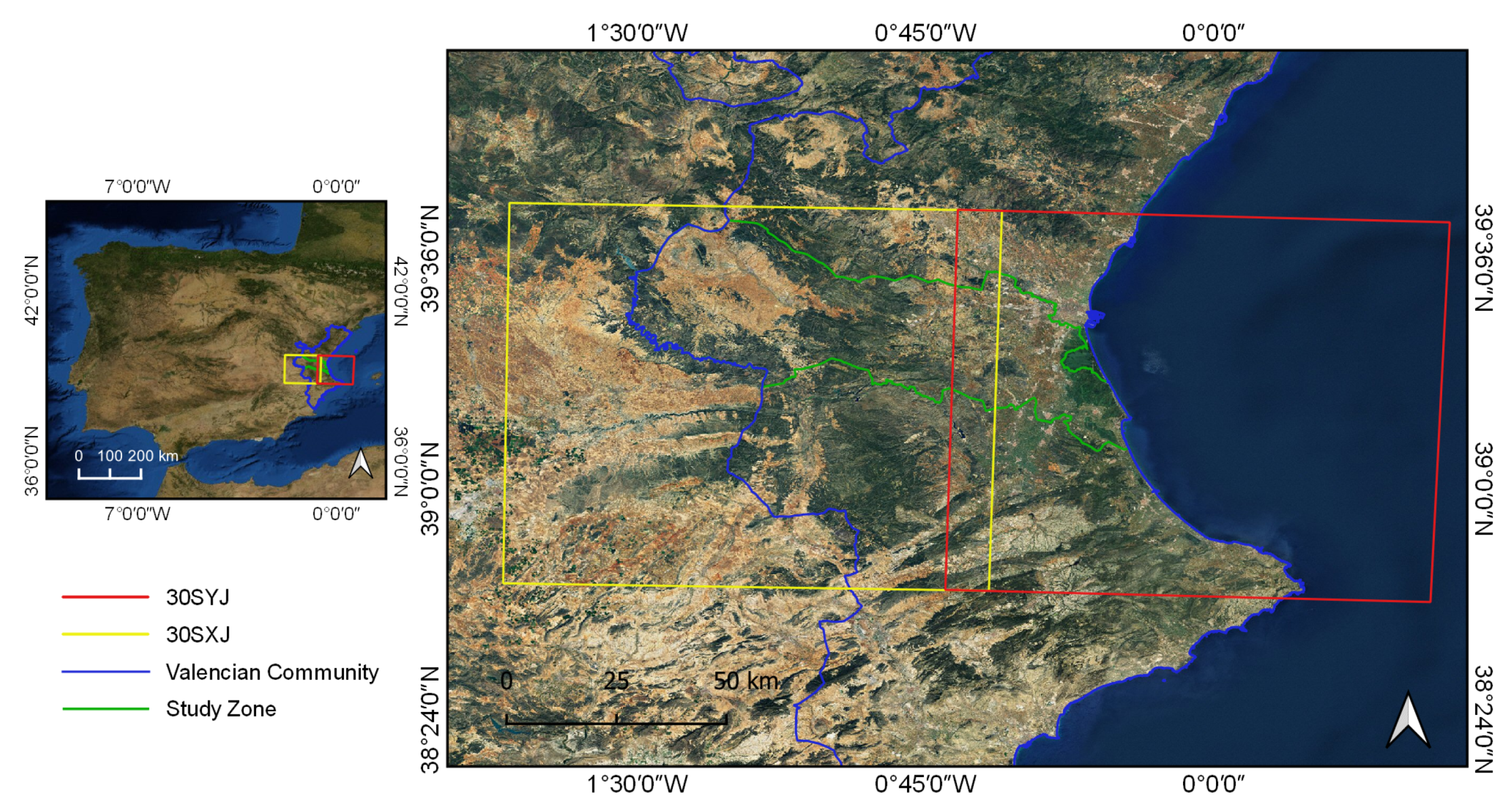
2.1. Study Area and Ground Truth

The study area of this work is located in the Valencia Community (East of Spain). It covers 344,600 ha and is observed by two Sentinel-2 tiles, 30SXJ and 30SYJ (see Figure 1). The typical climate of this region is Mediterranean, with an average temperature and humidity of 18 °C and 65%, respectively.

Ground truth was provided by regional Valencian authorities (see

Table 1. Ground truth: number of pixels for every class.

	VI	AL	FV	FR	OL	CI	DF	VO	Total
Abandoned	16,547	1619	812	159	86	1756	566	188	21,733
Active	20,000	20,000	2023	12,707	3083	20,000	20,000	1555	119,742

). Two major classes of parcels were considered: active and abandoned, both of them containing the following 8 subclasses: Vineyards (VI), Arable Land (AL), Fruits-Vineyard (FV), Fruits (FR), Olive grove (OL), Citrus (CI), Dried Fruit (DF) and Vineyard-Olive grove (VO). This database has been built by expert technical agronomists through several in-situ inspections in 2018.

2.2. Sentinel-2 Data

Sentinel-2 images were downloaded through the Google Earth Engine (GEE) platform. This platform provides a planetary scale catalogue of peta-bytes of images from several missions that can be accessed freely. Sentinel-2 provides imagery every 5 days, and carries on board a spectral sensor called MultiSpectral Instrument (MSI). MSI allows to acquire images in 13 spectral bands distributed in the spectral range of 443 nm to 2190 nm, however, data from the band 10 (cirrus band) was excluded as it does not provide relevant ground information. The features of the used bands are shown in

Table 2. Sentinel-2 bands used in the study.

Band	Central $\mathit{\lambda }$ (nm)	Bandwidth (nm)	Spatial Resolution (m)
B1	443	21	60
B2	492	66	10
B3	560	35	10
B4	665	31	10
B5	705	15	20
B6	740	15	20
B7	783	20	20
B8	842	106	10
B8A	865	21	20
B9	945	20	60
B11	1610	90	20
B12	2190	180	20

. Concretely, the level 2A product, which provides top-of-canopy surface reflectance data was used. Altogether, 67 cloud-free images from 26 May 2017 to 11 March 2020 were included.

2.3. Spectral Indices

Five spectral indices (SI) were considered for assessing the temporal differences between abandoned and active parcels. The selected indices were:

• Normalized Vegetation Difference Index (NDVI). This vegetation index is a normalized difference between near-infrared and red reflectance:

  $$NDVI=\frac{B_8-B_4}{B_8+B_4}.$$

  (1)
  It is sensitive to chlorophyll content, water content and vegetation fraction cover. Thus, it has been used for widely for remote sensing applications, including vegetation phenology monitoring [14], vegetation productivity, and also NDVI time series had been used before to distinguish cropland abandonment from fallow [8].
• Soil Adjusted Vegetation Index (SAVI) [15]. In scenarios with intermediate levels of vegetation coexisting with soil, the SAVI minimizes the brightness produced by the latter. SAVI is defined as

  $$SAVI=\frac{B_8-B_4}{B_8+B_4+L}\times (1+L),$$

  (2)

  and allows to describe a wider range of canopies with intermediate vegetation, by introducing the soil correction factor L, which depends on the fractional vegetation cover. In this work, L was set to $0.5$, an intermediate value that works well in the majority of scenarios.
• Normalized Burn Ratio (NBR) [16]. This SI is built as a normalized difference between near-infrared and short wave infrared reflectance:

  $$NBR=\frac{B_8-B_{12}}{B_8+B_{12}}.$$

  (3)
  NBR is related with the vegetation water content. It has been widely used in wildfire severity mapping, but recently it has been also used to detect drastic reductions in vegetation biomass, for example when crops are harvested.
• Bare Soil Index (BSI) [17]. This spectral index results from a combination of NDVI and Normalized Built, which is a bare soil index. In terms of the bands of Sentinel-2,

  $$BSI=\frac{(B_{12}+B_4)-(B_8-B_2)}{(B_{12}+B_4)+(B_8-B_2)}$$

  (4)
  BSI varies from −1 to 1, taking higher values where there is higher soil bareness.
• Red edge chlorophyll index (CI_re). The selected chlorophyll index [18] is defined as

  $$C{I}_{re}=\frac{B_7}{B_5}-1$$

  (5)

  in terms of Sentinel-2 bands. This ratio has proven to be more precise in estimating chlorophyll content than other Sentinel-2 indices [19].

2.4. Interclass Separability

In this study, the Jeffries–Matusita (JM) and Bhattacharyya (BH) [20] distances were used to evaluate the class separability. The JM distance allows to quantify the similarity between samples of two distributions and is defined as

$$J_{ij}=2(1-e^{-B_{ij}})$$

(6)

where $B_{ij}$ is the multivariate Bhattacharyya distance,

$$B_{ij}=\frac{1}{8}{({\mu }_j-{\mu }_i)}^t{\left[\frac{{\Sigma }_i+{\Sigma }_j}{2}\right]}^{-1}({\mu }_j-{\mu }_i)+\frac{1}{2}ln\left(\frac{|{\Sigma }_i+{\Sigma }_j|/2}{\sqrt{|{\Sigma }_i\left|\right|{\Sigma }_j|}}\right)$$

(7)

where ${\mu }_i$, ${\mu }_j$ are the mean vectors of the classes and ${\Sigma }_i$, ${\Sigma }_j$ their covariance matrices. JM distance is constrained in the interval $[0,2]$, so when two classes are totally separated the JM distance is 2. Moreover, if $1.9<\mathrm{JM}<2.0$ we consider that separability is good, $1.8<\mathrm{JM}<1.9$ corresponds to intermediate separability, and $\mathrm{JM}<1.8$ to poor separability [21].

2.5. Machine Learning and Deep Learning

A range of classifiers were used for classifying land uses and abandoned parcels. They include the Linear Discriminant Analysis (LDA) and Quadratic Discriminant Analysis (QDA), which fit a gaussian distribution to each class of the training data, and then assigns an incoming observation of the class with maximum posterior probability. The difference between these two methods is that the covariance matrices of LDA are independent of the class while for QDA the covariance matrices are class-dependent. Non-parametric classifiers like k-NN, Decision Trees (DT) and Random Forest (RF) were also trained. k-NN [22] is a simple but effective algorithm that assigns a new observation to the most frequent class among the k-nearest neighbours, according to a distance measurement (e.g., Euclidean or Mahalanobis distances) in the feature space. A DT is a set of hierarchical rules that splits the feature space in subsets [23]. The rules are thresholds set over the features, with the goal of maximizing the purity (or entropy) of the resultant subsets. RF is an ensemble algorithm based on training a forest of DTs with randomly selected features (predictors) and randomly selected samples [24]. Random selection of samples and features, as well as the voting of multiple DTs, result in robustness against noisy observations and usually competitive accuracies.

Two deep learning models were also trained, specifically, a Long Short Term Memory (LSTM) network and its bi-directional version (BiLSTM). LSTM is a special type of Recurrent Neural Network (RNN) designed to deal with the problem of the vanishing gradient, and learn long-term dependencies [25]. This special architecture is well suited to deal with sequential data, like the RS time series considered in this study. Every LSTM cell contains three gates that control the information flow and decide its relevance: the input gate (${\mathbf{i}}_t$), forget gate (${\mathbf{f}}_t$), and output gate (${\mathbf{o}}_t$). At a time step t, one hidden unit receives the input data ${\mathbf{x}}_t$, and the previous hidden state ${\mathbf{x}}_{t-1}$. Its combination is modulated by an hyperbolic tangent,

$${\tilde{\mathbf{c}}}_t=tanh({\mathbf{W}}_c{\mathbf{x}}_t+{\mathbf{U}}_c{\mathbf{h}}_{t-1}+{\mathbf{b}}_c)$$

(8)

where ${\mathbf{W}}_c$, ${\mathbf{U}}_c$, y ${\mathbf{b}}_c$ are the initial weights, the recurrent weights and the bias, respectively. A sigmoid-like input gate decides which of the information is stored in the cell,

$${\mathbf{i}}_t=\sigma ({\mathbf{W}}_i{\mathbf{x}}_t+{\mathbf{U}}_i{\mathbf{h}}_{t-1}+{\mathbf{b}}_i)$$

(9)

and similarly, the forget gate decides which information is removed from the current cell state.

$${\mathbf{f}}_t=\sigma ({\mathbf{W}}_f{\mathbf{x}}_t+{\mathbf{U}}_f{\mathbf{h}}_{t-1}+{\mathbf{b}}_f)$$

(10)

The memory cell is updated by adding information coming from input gate and forget gate, which means that new information is given by ${\mathbf{c}}_t$, and part of the information at the current memory is discarded,

$${\mathbf{c}}_t={\mathbf{i}}_t\odot {\tilde{\mathbf{c}}}_t+{\mathbf{f}}_t\odot {\mathbf{c}}_{t-1}$$

(11)

Eventually, the output hidden state results from a combination of the output gate and the updated memory cell,

$${\mathbf{h}}_t={\mathbf{o}}_t\odot tanh\left({\mathbf{c}}_t\right)$$

(12)

where the output gate ${\mathbf{o}}_t$ is given by

$${\mathbf{o}}_t=\sigma ({\mathbf{W}}_o{\mathbf{x}}_t+{\mathbf{U}}_o{\mathbf{h}}_{t-1}+{\mathbf{b}}_o)$$

(13)

LSTM units can be combined in order to obtain a BiLSTM network. These units are composed of two LSTM units at each time step, and have in consideration both past and future hidden states, meaning that BiLSTM networks learn from the full time series at each iteration [26]. In this work, we trained LSTM and BiLSTM networks with the following architecture:

• One entry layer containing the 67 Sentinel-2 images with 13 predictors.
• Two layers of neurons with 100 hidden units, each one followed by a 50% dropout layer to avoid overfitting.
• One fully connected layer connecting the activation functions from the hidden units to the following layer.
• One softmax layer that computes the probability assigned by the network for each class.
• Output layer with the final predictions.

2.6. Experiments

Firstly, the temporal behaviour of the selected spectral indices was compared to investigate possible differences in the temporal evolution of indices over abandoned and non-abandoned lands. This leads to a first approximation of knowledge about the abandonment scenario. Then, the JM distance was computed in order to assess the separability among pairs of classes (including abandoned and non abandoned). The average distance between every pair of classes was computed. It was also evaluated how the separability increases as more images are stacked to the feature space, which is more representative of the inter-class separability since the predictors used for the classification are the full time series.

Finally, and according to the two major classes (abandoned and active) and the 8 sub-classes, three different classification tasks (using the ML and DL algorithms listed in Section 2.5) were considered to evaluate the Sentinel-2 capabilities over all three scenarios:

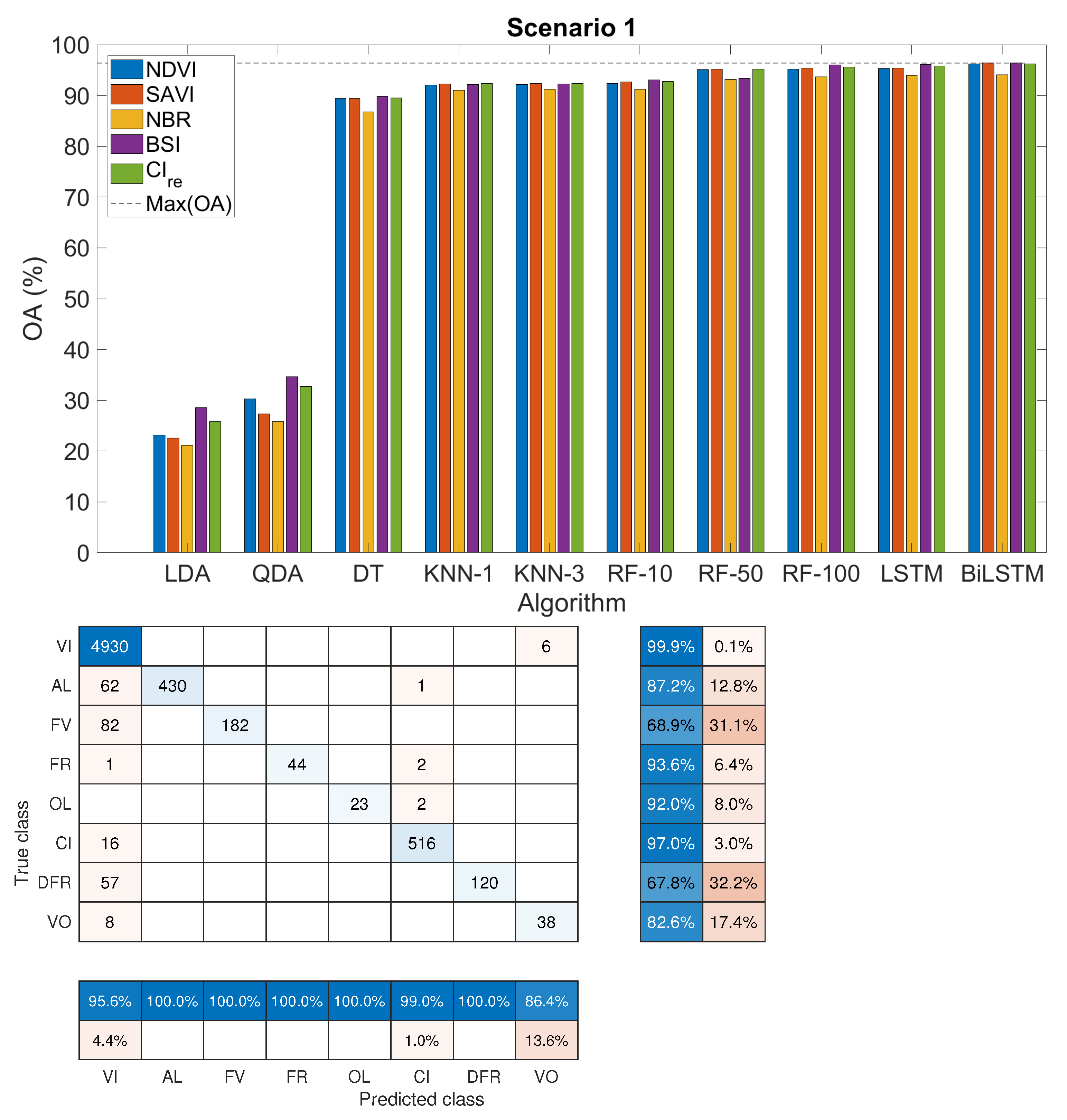
• Scenario 1: we considered only the eight subclasses for the abandoned parcels. This problem is related to the ability to identify the former crop type of the abandoned field.
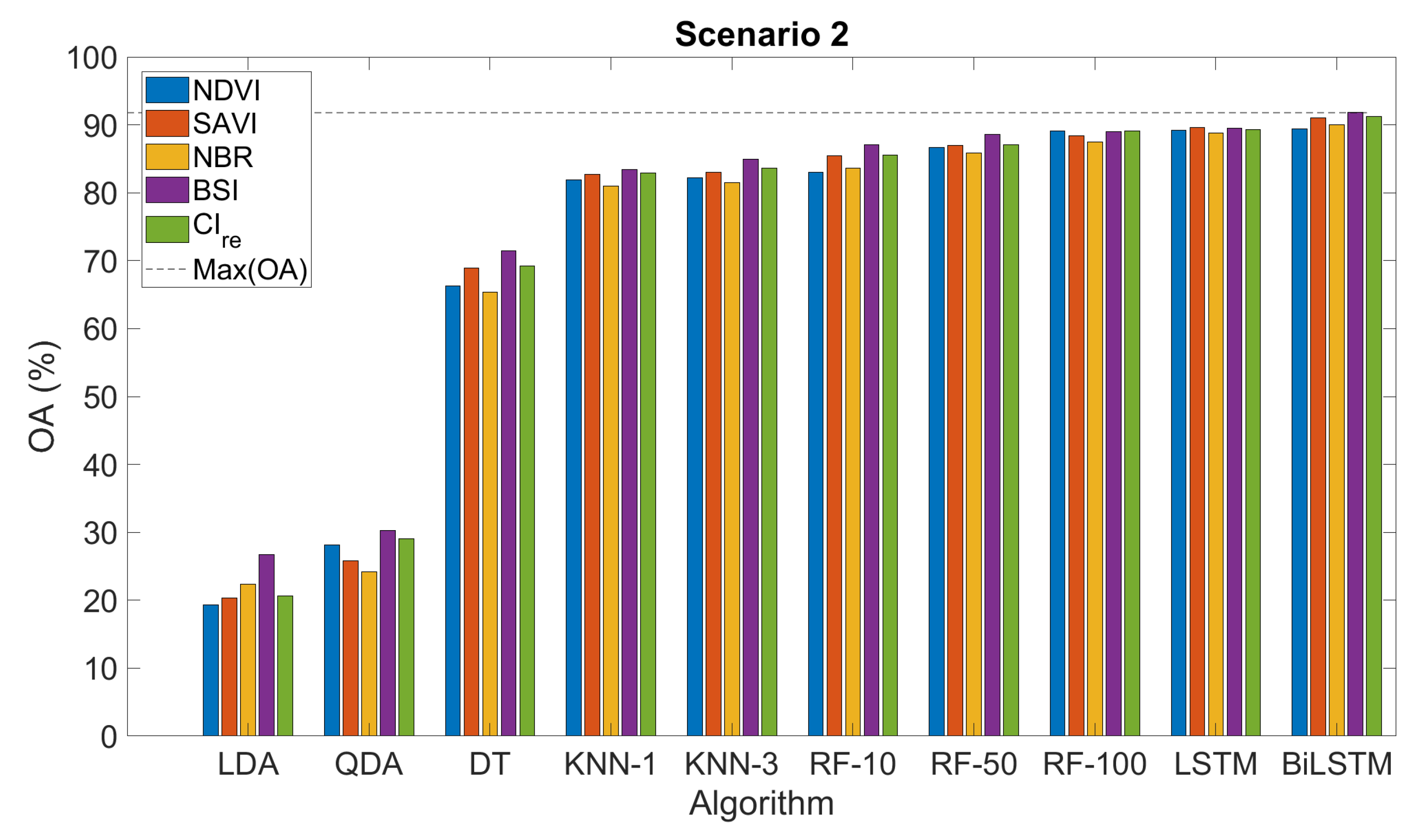
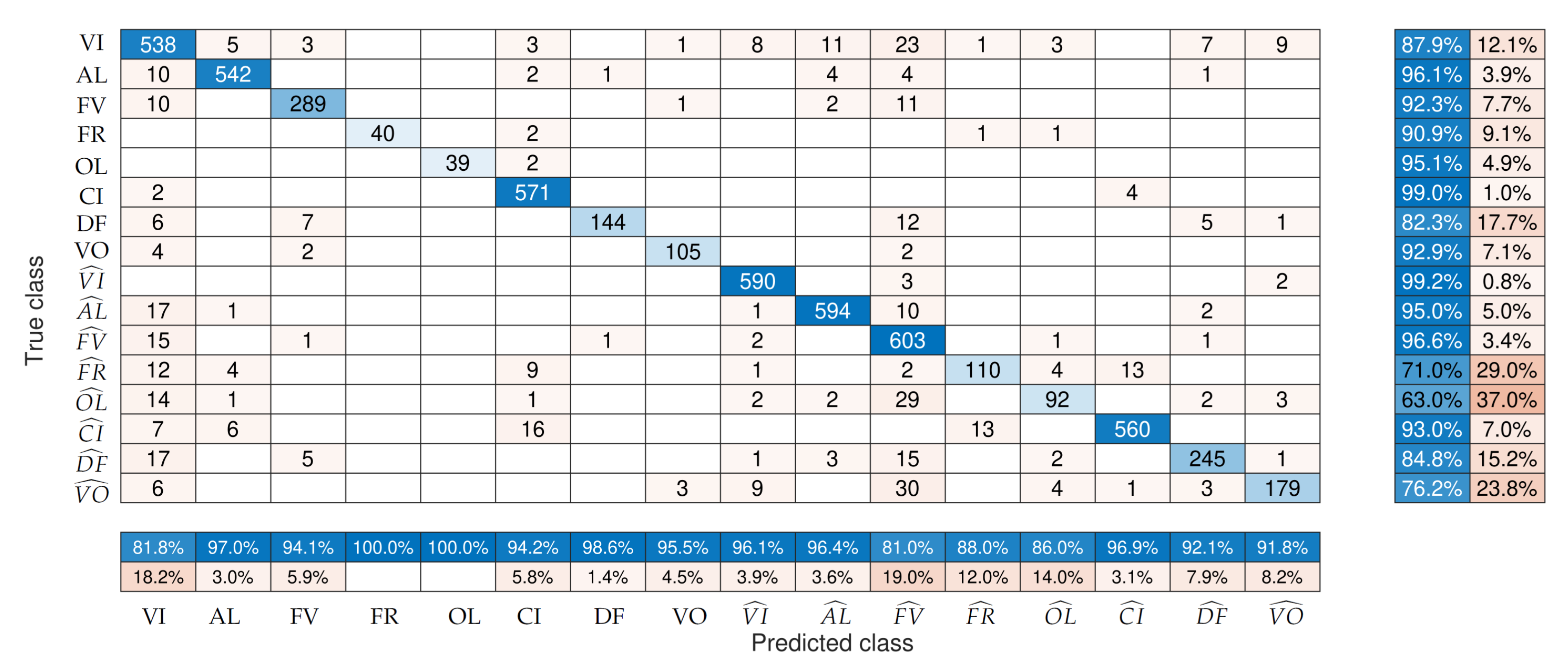
• Scenario 2: we considered all classes, i.e., eight classes of active parcels and their respective eight classes of abandoned fields. This is on paper the hardest scenario, where we aimed to distinguish abandoned from active cropland and distinguish every crop type.
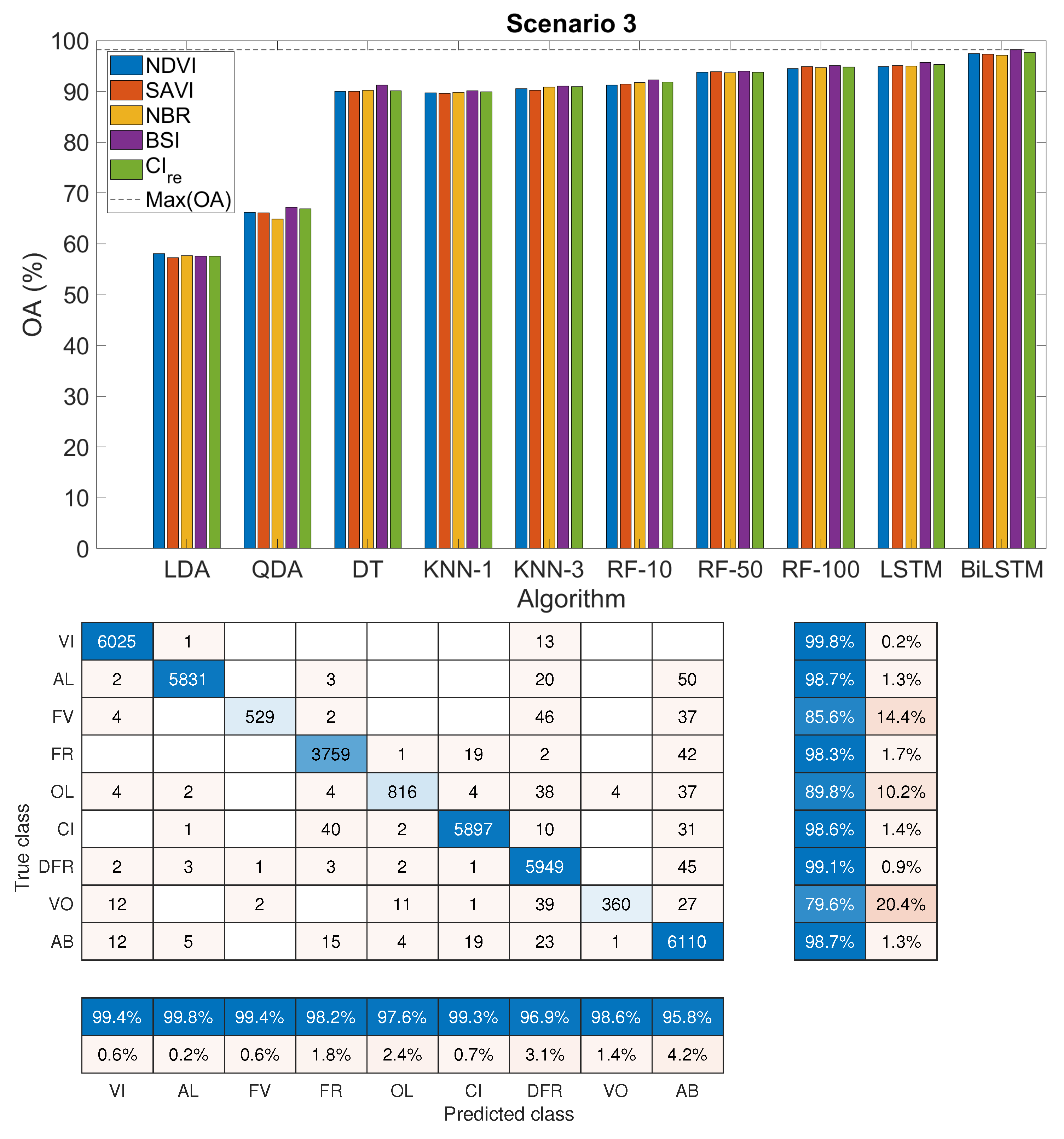
• Scenario 3: we considered eight classes of active land and one major class containing all the abandoned samples.

For every task and classifier, a dataset of dimensions ($n\times 13\times 67$), corresponding respectively to the number n of samples, the number of predictors, and the number of Sentinel-2 images used in the study was built. The first twelve predictors are the Sentinel-2 reflectance bands, and the last one corresponds to one of the spectral indices described in Section 2.3. Then, every dataset was split in two subsets, one corresponding to the 70% of the samples for training the models, and the remaining 30% used to test the accuracy of the models (see Section 3.3). This is the preferred split selection when there is enough available reference data.

3. Results

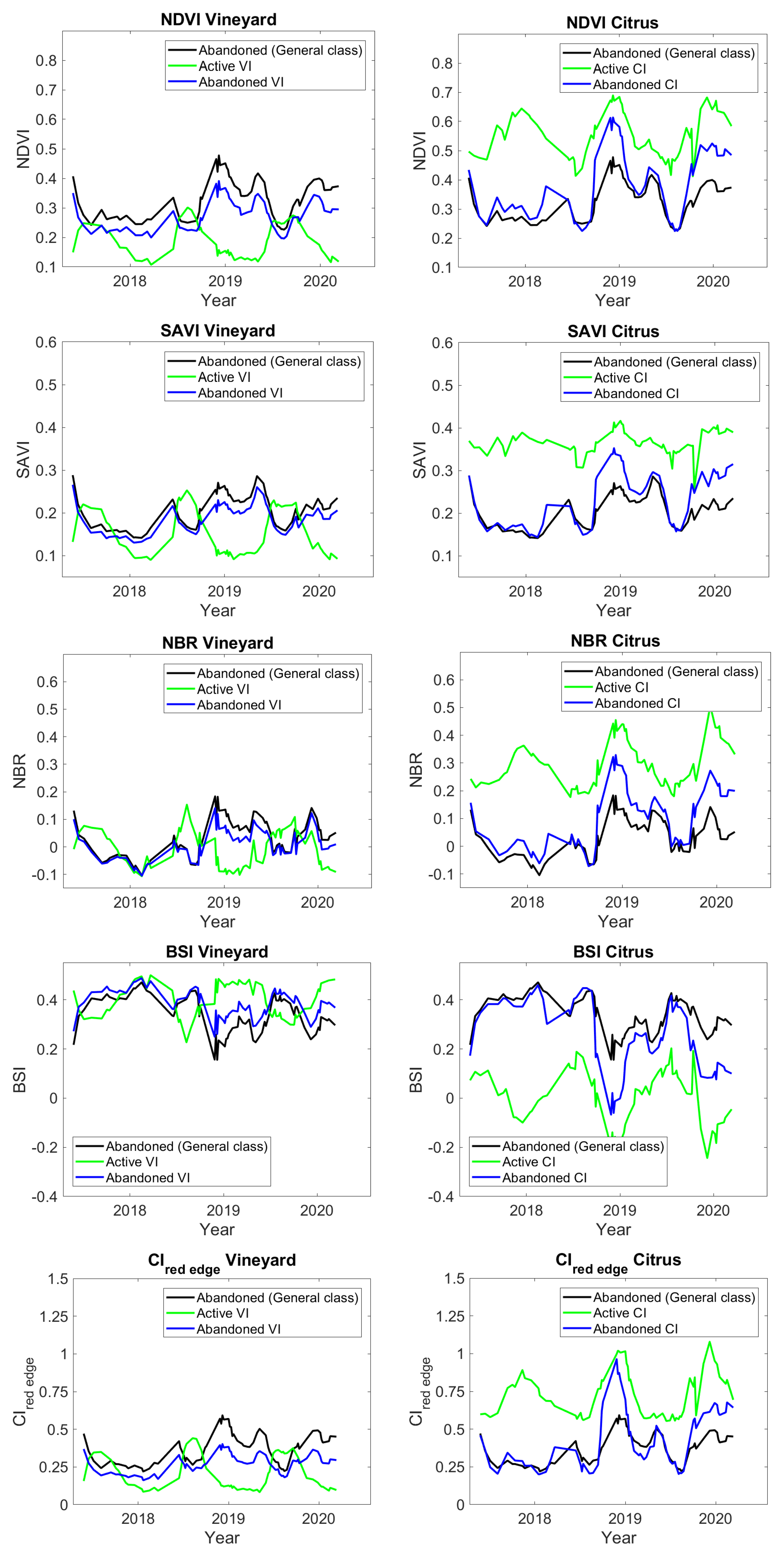
3.1. Spectral Indices Time Series

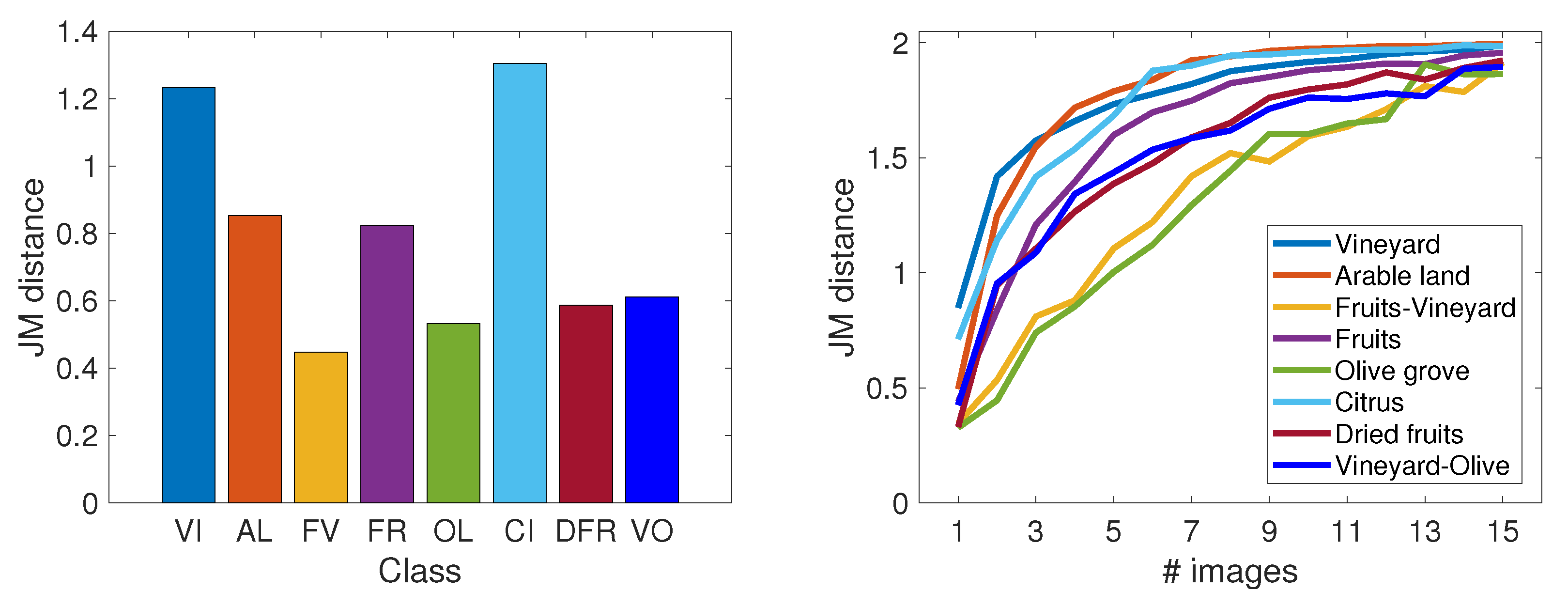
In this section, we show the temporal behaviour of selected spectral indices over abandoned and active parcels. For the sake of brevity, we only show two of the most representative classes, vineyard and citrus (Figure 2). From VI time series, one observes that the phenological profile of the abandoned classes and the active one are shifted with respect to active crops. This suggests that new vegetation species appear in the parcel once it is abandoned, allowing to differentiate better between abandoned and active crops. Another feature of vegetation that allows to differentiate cropland from scrubs is fraction of vegetation cover (FVC). For instance, arable land parcels have strong seasonal variations due to high FVC, which results in higher separability from abandoned crops. Lastly, SIs values of CI are high throughout all the year (or lower, for BSI), which can be the main reason for the high separability of abandoned classes, using either single images or multitemporal inputs.

On the other hand, classes where the senescence periods from the active class and scrubs do not differ greatly, or FVC is not especially high, may be less likely to be well distinguished, being the case for OL, VO, and DF.

3.2. Separability

Results for separability analysis are shown in

Table 3. JM distances between considered classes. The upper part shows the JM distances obtained after stacking 15 Sentinel-2 images, while in the lower part the average distance for the 67 images is shown. On the other hand, VI stands for abandoned Vineyard, while $\widehat{VI}$ stands for the corresponding active class, following the same distinction for the rest of the classes.

	VI	AL	FV	FR	OL	CI	DF	VO	$\widehat{\mathit{VI}}$	$\widehat{\mathit{AL}}$	$\widehat{\mathit{FV}}$	$\widehat{\mathit{FR}}$	$\widehat{\mathit{OL}}$	$\widehat{\mathit{CI}}$	$\widehat{\mathit{DF}}$	$\widehat{\mathit{VO}}$
VI		1.96	1.97	2.00	2.00	1.99	1.91	2.00	1.96	2.00	1.84	1.97	1.83	1.98	1.90	1.87
AL	0.59		1.99	2.00	2.00	1.98	1.99	2.00	2.00	2.00	1.97	1.97	1.98	1.99	1.99	1.99
FV	0.50	0.98		2.00	2.00	2.00	1.93	1.97	2.00	2.00	1.87	2.00	1.99	2.00	1.99	1.99
FR	1.29	1.46	1.40		2.00	2.00	2.00	2.00	2.00	2.00	2.00	2.00	2.00	2.00	2.00	2.00
OL	0.99	1.24	1.15	1.18		2.00	2.00	2.00	2.00	2.00	2.00	2.00	2.00	2.00	2.00	2.00
CI	1.00	1.04	1.33	1.19	1.12		2.00	2.00	2.00	2.00	2.00	2.00	2.00	1.99	2.00	2.00
DF	0.58	0.86	0.44	1.50	1.27	1.42		1.99	2.00	2.00	1.89	2.00	1.99	2.00	1.98	1.98
VO	0.79	1.26	0.71	1.57	1.29	1.51	0.80		2.00	2.00	2.00	2.00	2.00	2.00	2.00	2.00
$\widehat{VI}$	1.18	1.55	1.34	1.89	1.75	1.77	1.36	1.36		2.00	1.98	2.00	1.99	2.00	1.97	1.97
$\widehat{AL}$	0.89	0.97	1.16	1.70	1.49	1.43	1.11	1.38	1.34		2.00	2.00	2.00	2.00	1.99	1.99
$\widehat{FV}$	0.45	0.87	0.49	1.56	1.30	1.39	0.47	0.89	1.11	1.03		2.00	1.76	1.99	1.89	1.88
$\widehat{FR}$	0.91	0.82	1.30	1.58	1.36	0.95	1.28	1.46	1.52	1.06	1.14		1.99	1.96	1.99	1.99
$\widehat{OL}$	0.60	0.77	0.79	1.49	1.21	1.17	0.72	1.09	1.30	0.98	0.38	0.93		1.99	1.96	1.93
$\widehat{CI}$	1.38	1.23	1.61	1.75	1.60	1.13	1.58	1.69	1.74	1.42	1.49	0.68	1.22		2.00	2.00
$\widehat{DF}$	0.59	0.96	0.67	1.60	1.35	1.39	0.61	0.98	0.98	0.86	0.45	1.18	0.66	1.51		1.93
$\widehat{VO}$	0.60	1.03	0.78	1.63	1.37	1.41	0.74	0.89	0.94	1.08	0.32	1.14	0.46	1.46	0.58

. The first 8 × 8 box accounts for JM distances between abandoned classes (e.g., VI − AL), which corresponds to the aforementioned scenario 1, meanwhile the full table corresponds to scenario 2. The corresponding active classes are denoted with an additional subscript (e.g., $\widehat{VI}-\widehat{AL}$). Since the JM are symmetric, the lower part of the table corresponds to the average distance between pairs of classes, and the upper part to the distances calculated when 15 images are stacked together.

The results show that when using single images, the obtained JM distances between pairs of classes are considerably lower than 1.8, meaning that the data distributions of the classes are highly overlapped. This is especially notorious for some classes, like VI, which presents high confusion with FS, $\widehat{DF}$, $\widehat{OL}$, and $\widehat{FV}$. FV is also highly overlapped with other classes like DF, VO, or $\widehat{FV}$. On the other hand, CI and OL show greater distances with the rest of the classes, noting that only single images were considered.

As expected, JM distances obtained with stacked images as inputs are much greater than those obtained with unitemporal inputs. For the majority of cases, JM is greater than 1.9, and close to 2, meaning that those pairs of classes are likely to be well distinguished by classification algorithms. The greater overlapping is found between $\widehat{FV}$ and $\widehat{OL}$, VI, FV, DF and $\widehat{VO}$ classes, with JM distances generally ranging from 1.8 to 1.9.

Lastly, the results for the third classification problem are shown in Figure 3, where the left panel shows the average JM distances between active classes and the abandonment class (AB) for unitemporal inputs. These indicate that unitemporal inputs are not enough to distinguish between samples from AB and the active crop classes. Special overlapping exists for FV, OL, FS and VO, while VI and CI are more differentiated, but still far from acceptable separability thresholds (i.e., 1.8). Otherwise, when we calculate JM distances for multitemporal inputs we find that the separability keeps increasing as more images are stacked together. This results in much greater JM distances, beyond the 1.8 limit for most pairs of classes (see Figure 3 (right)). Similarly to the unitemporal case, VI, CI and AL are the classes with higher distinction, while OL, FV, VO and DF appear to be more overlapped with AB. Another relevant finding here is the importance of the dates chosen to calculate the distances, since the average distance shown in Figure 3 (left) is greater than the first JM distance in Figure 3 (right) for some classes (e.g., CI) and lower for others (e.g., VO). This is related to the phenological state of vegetation in the date of selection, therefore, we selected images covering the complete phenological cycle for the calculation of stacked JM distances.

In all cases, these results reinforce the need to use multitemporal reflectance data as an input to differentiate between crop types, and abandoned parcels.

3.3. Classification Accuracy

We assessed the performance of every algorithm based on the overall accuracy (OA) obtained in the test set. Also, for the best performing algorithm and dataset we computed the confusion matrix, i.e., a double entry table where row entries represent the actual classes (labels in the testing data) and column entries the predicted classes.

For scenario 1 (Figure 4), the obtained accuracies are high (OA $>89\%$), except for the parametric classifiers (LDA and QDA). The best performing algorithms are RF with 100 trees (RF-100), and deep LSTM and BiLSTM networks, with accuracies higher than $95\%$, with the best case being the model obtained with BiLSTM and the BSI dataset, with a $96.4\%$ OA. We also noted that in this first problem, all the indices performed similarly. However, NBR showed slightly lower OA values (1–2%) than the other models, which could be attributed to the higher similarity of the NBR temporal profiles for all the abandoned crops. The per-class User Accuracy (UA) values were high, with the exception of the VO class (86.4%). The lowest per-class Producer Accuracy (PU) values were found in DF, FV and AL classes (with 67.8%, 68.9% and 82.6% PU, respectively). These classes present large omission errors due to incorrect assignations to VI, the class with the highest number of samples.

Lower accuracy values were achieved in the most challenging problem (scenario 2, Figure 5) considering eight classes of abandoned fields. In this case, we obtained the highest accuracy with BiLSTM trained with the BSI dataset, resulting in $91.8\%$ OA, whereas the accuracies of the remaining algorithms were below 90%. Here, the confusion is higher among active crop classes, with lower UA and PA for FV, DF, OL and VO, and also active vineyards.

Lastly, in Figure 6 we show the results for scenario 3. Here, we considered active crops, and a general class of abandoned ones (denoted as AB). In this case, we obtained the best performing approaches. In particular, for the BiLSTM network trained with BSI and CI_re we obtained OAs of $98.2\%$ OA and $97.6\%$, respectively. Moreover, UA are high in the majority of cases. The lowest PA was found in OL, FV and VO classes (89.8%, 85.6% and 79.6%, respectively). The higher rate of omission errors in these classes could be explained by (1) class imbalances in the training dataset (i.e., fewer samples of OL, FV and VO), and (2) higher spectral confusion among these classes. This confusion was observed in the previous separability analysis, revealing that OL, FV and VO are classes with less distinctive seasonal variations in comparison with CI, VI or AL.

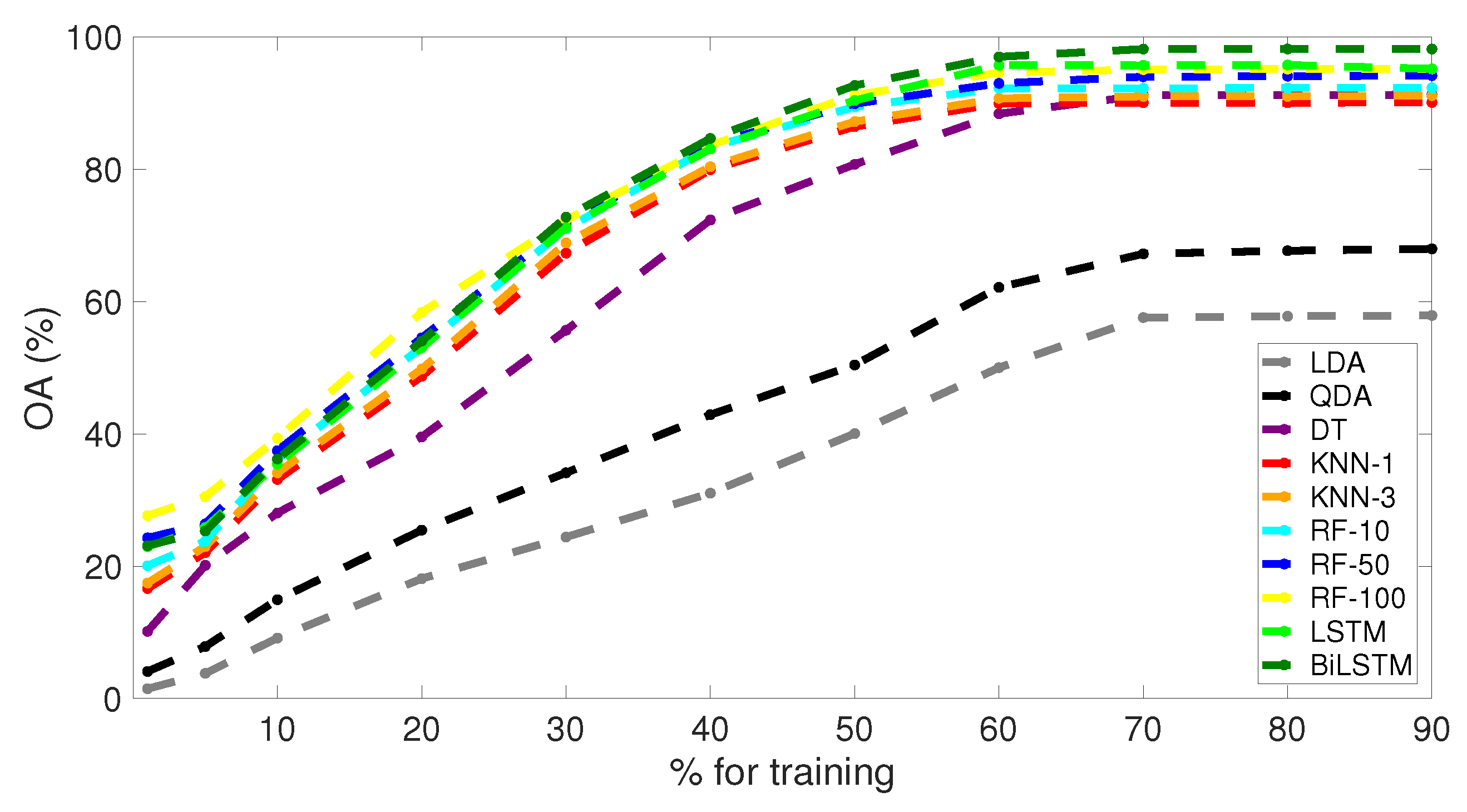
3.4. Effect of Dataset Training Size

The higher misclassification rates found in the classes that were poorly represented in the training data shows the importance of feeding well constructed datasets into the algorithms. In the latest case, the ones that benefit most from this feature (i.e., LDA-QDA, DT and LSTM-BiLSTM) showed much better performance, with suggests that in scenario 3 we reached the optimal configuration in terms of considered classes. As a final experiment, we tested the role of training dataset size (Figure 7) in the best case scenario (i.e., scenario 3 using the 2-BiLSTM trained with the BSI dataset).

The results show that when using small training datasets, RF-100 performs better than deep architectures. However, LSTM and especially BiLSTM networks outperform the rest of algorithms when an increased number of training data is available.

4. Discussion

Land use classification of agricultural cropland admits several approaches in terms of data selection and methodology, in order to distinguish every vegetation cover. One approach is, for instance, to calculate temporal series of a spectral index and handcraft a model with parameters that describe the temporal variations of the vegetation over the year, which are caused by senescence. Then the parameters are adjusted for every class and new observations are identified with the models that better describe their variations. However, this approach is limited limited for a number of reasons: (i) requirement of expert knowledge to handcraft the best possible model; (ii) need of a rigorous pre-processing chain to detect possible outliers that confuse the model; (iii) while using vegetation indices, the full information contained in images is under-exploited.

Other approach (the one used in this work) consists of acquiring large temporal series that also describe vegetation senescence, and then using these as inputs for supervised classification. Some studies have shown that a relatively small set of images properly distributed in time can be sufficient to obtain high accuracies [4]. Since temporal resolution of recent satellites (e.g., Landsat 8, Sentinel missions) has increased, this is not a problem anymore and usually multitemporal approaches are now preferred over single observation ones. Also, some studies have shown that data fusion of reflectances with other sources like Radar or Lidar can be beneficial in order to improve results [5]. Lastly, it is worth mentioning the rise of deep learning as an alternative over more traditional machine learning methods. Results show that recurrent neural networks can be used successfully to classify remote sensing sequential data [10,11].

Regarding the case of land abandonment, there are studies relying on handcrafted models to detect abandoned croplands [8], and also others based on supervised classification [6,27]. In previous works related to abandonment detection in the Valencian Community, single orthophotos (0.25 m spatial resolution) have been used to identify abandoned citrus crops [28], whereas in the present study we have shown that a different approach relying on multitemporal Sentinel-2 data (10 m spatial resolution and 5-day revisit time) is possible. The proposed methodology uses machine learning and state-of-the-art deep learning classification methods, and offers a number of advantages for its use. Sentinel-2 MSI has a rich spectral signature that allows to monitor land cover and vegetation dynamics [29,30]. With our approach, it is possible to fully exploit these capabilities, along with spectral indices for enhancing the class discrimination. Fully exploiting temporal and spectral information of Sentinel-2A and 2B has led to very high accuracies in detecting abandoned crops over a large area.

The high temporal frequency of Sentinel-2 (around 70 images per year) was enough to capture the temporal behaviour of classes. On the other hand, improved spatial resolution of these satellites (in comparison to MODIS) has allowed us to perform this type of identification task in a study zone like the Valencian province, where the average parcel is small (5 ha). Moreover, we have adopted a pixel-based classification strategy, while it is also possible to perform object-based classification. This approach often requires an additional preprocessing, consisting of the image segmentation in compact, connected objects (e.g., parcels). The authors of [31] performed a comparison between object-based and pixel-based crop identification, finding that an object-based approach does not necessarily improve accuracy, while a pixel-based one is more efficient in terms of computation. On other side, CAP regulations contemplate the possibility of partial abandonment, where only a fraction of the parcel is unsuited for agricultural activity. Thus, it is reasonable to opt for pixel-based detection of abandonment, since it can be useful for later assessment of partial subsidies in semi-abandoned crops.

Abandonment can be caused by many different factors, and result in different outcomes. When the land is left unused, the parcels are slowly invaded by the local ecosystem. This implies that the results of land abandonment can be very different depending on the environmental conditions of the region. In our study zone, it is common that land abandonment results in parcels covered by abundant shrubs. In our work, we have studied the temporal profiles of abandoned and active crops for all considered classes. While active classes can be distinguished according to some particular traits like senescence and FVC, abandoned ones show a much more similar behaviour, in fact similar to the one expected for shrubs. This allows to distinguish active from abandoned classes, with higher accuracies for crops with very distinctive variations in terms of phenological parameters and vegetation cover (e.g., VI and CI crops).

For all the considered scenarios, OA is higher than 90% in the best case performance. Moreover, the results show that, among the considered spectral indices to be included as a 13th predictor, BSI is the one that reports the best results. On the other hand, NBR shows the lowest performance, especially in the first experiment, where we only considered abandoned crops. This can be explained by the similarity of temporal profiles in all abandoned subclasses. However, NBR is useful to distinguish between active and abandoned crops (scenarios 2 and 3). This can be explained by the different phenological variations that grasslands and shrubs show in comparison to cropland. While the latter sometimes suffer from variations induced by agronomical practices (e.g., harvesting), grasslands present natural phenological patterns due to seasonal and meteorological effects [32]. With respect to the SIs built around visible red-edge and NIR, performance is similar, with slightly higher accuracies for CI_re, which suggests that red-edge information can be useful and it could be worth including an NDVI or SAVI version using red-egde bands.

Another point to discuss is the fact that we can associate a higher number of misclassifications of classes under-represented in the training dataset (i.e., minority or rare classes). It is well known that in classification problems, a key aspect is disposing of abundant, well balanced and representative samples datasets, since many algorithms fail when these conditions do not exist. If the training dataset presents imbalances between classes and does not reflect the actual population, it can lead to a big bias in classification, i.e., in scenario 1, where we obtained some commission errors in VI class. We noticed that this fact is not caused by overlapping between VI and the rest of the classes, but by the over-representation of VI in the training dataset. In scenarios 2 and 3, we aimed to correct the imbalances by down sampling some of the majoritarian classes, obtaining results that are more consistent with previous separability study. Although acquiring sufficient ground truth data is one of the major problems in remote sensing classification tasks, we conclude that for future studies more field work would be required to reduce sampling bias by improving the statistical representativity of minority classes.

There is another potential issue that we identified before the study, also related with the database, since it corresponds to the 2018 update. The abandoned fields could have been left unused just before the check inspection, or been in that state for some years. We supposed that this could be problematic because it might happen that two parcels corresponding to the same class could be in different stages of degradation. Based on the obtained results, this is something that either has not happened, or if has happened our temporal series were larger enough to distinguish the majority of abandoned crops, especially in scenario 3. However, this opens a question on how to detect future abandonments as early as possible. This is a slightly different problem that could may be approached from an anomaly detection perspective [33], and where the temporal resolution of Sentinels can play an important role.

Lastly, with respect to the algorithms used in the study, we observed that in this particular classification task deep learning architectures were able to extract the most information from the training data, and achieved the highest accuracy in all the proposed experiments. This was especially the case in the third scenario, where training datasets disposed the abundant samples for the majority of classes. It is worth mentioning that in this scenario, BiLSTM overall accuracy was 2% higher than LSTM one. The fact that this network is able to learn from both past and future states in such a complex way is something that can set it apart from the rest of the classification algorithms. However, random forest performed even better than deep learning architectures in scenarios with limited training data, being a good alternative to DL algorithms.

5. Conclusions

In this work, the Sentinel-2 capabilities were assessed to detect cropland abandonment in the Valencian Community in Spain. The methodology is based on building multitemporal datasets based on Sentinel-2 reflectances and derived spectral indices. Time profiles of spectral indices revealed differences in the temporal behaviour of abandoned lands and active classes. In addition, three classification experiments using machine learning and deep learning algorithms fed by different number of classes were undertaken.

The results reported good accuracies for all experiments, being able to distinguish the majority of samples with the selected classification algorithms. The considered deep learning techniques outperformed the machine learning algorithms when large datasets were used. In the case of reduced data for the training process, the random forest is able to perform at the same level, and even better than the deep learning techniques. The best case scenario was found when a BiLSTM was used for classifying eight classes of active crops and one class containing abandoned parcels. In this case, the predictors were the twelve Sentinel-2 bands plus the bare soil index, and the BiLSTM network reported an OA of $98.2\%$. This scenario is optimal in terms of class configuration, since it allows to distinguish the main active crops in the Valencia Community and also detects abandoned parcels. The proposed methodology could potentially be implemented in an automated procedure to supervise the CAP requirements to access subsidies.

References

1. European Union. Commission Implementing Regulation (EU) No 1306/2013 of the European Parliament and of the Council of 17 December 2013 on the financing, management and monitoring of the common agricultural policy and repealing Council Regulations (EEC) No 352/78, (EC) No 165/94, (EC) No 2799/98, (EC) No 814/2000, (EC) No 1290/2005 and (EC) No 485/2008. Off. J. Eur. Union 2013, 56, 1–59. [Google Scholar]
2. European Union. Commission Implementing Regulation (EU) 2018/746 of 18 May 2018 amending Implementing Regulation (EU) No 809/2014 as regards modification of single applications and payment claims and checks. Off. J. Eur. Union 2018, 61, 1–7. [Google Scholar]
3. Estrada, J.; Sánchez, H.; Hernanz, L.; Checa, M.J.; Roman, D. Enabling the Use of Sentinel-2 and LiDAR Data for Common Agriculture Policy Funds Assignment. ISPRS Int. J. Geo-Inf. 2017, 6, 255. [Google Scholar] [CrossRef] [Green Version]
4. Sitokonstantinou, V.; Papoutsis, I.; Kontoes, C.; Lafarga Arnal, A.; Armesto Andrés, A.P.; Garraza Zurbano, J.A. Scalable parcel-based crop identification scheme using Sentinel-2 data time-series for the monitoring of the common agricultural policy. Remote Sens. 2018, 10, 911. [Google Scholar] [CrossRef] [Green Version]
5. Campos-Taberner, M.; García-Haro, F.J.; Martínez, B.; Sánchez-Ruíz, S.; Gilabert, M.A. A copernicus Sentinel-1 and Sentinel-2 classification framework for the 2020+ European common agricultural policy: A case study in València (Spain). Agronomy 2019, 9, 556. [Google Scholar] [CrossRef] [Green Version]
6. Yin, H.; Prishchepov, A.V.; Kuemmerle, T.; Bleyhl, B.; Buchner, J.; Radeloff, V.C. Mapping agricultural land abandonment from spatial and temporal segmentation of Landsat time series. Remote Sens. Environ. 2018, 210, 12–24. [Google Scholar] [CrossRef]
7. Foerster, S.; Kaden, K.; Foerster, M.; Itzerott, S. Crop type mapping using spectral–temporal profiles and phenological information. Comput. Electron. Agric. 2012, 89, 30–40. [Google Scholar] [CrossRef] [Green Version]
8. Estel, S.; Kuemmerle, T.; Alcántara, C.; Levers, C.; Prishchepov, A.; Hostert, P. Mapping farmland abandonment and recultivation across Europe using MODIS NDVI time series. Remote Sens. Environ. 2015, 163, 312–325. [Google Scholar] [CrossRef]
9. Campos-Taberner, M.; Romero-Soriano, A.; Gatta, C.; Camps-Valls, G.; Lagrange, A.; Le Saux, B.; Beaupere, A.; Boulch, A.; Chan-Hon-Tong, A.; Herbin, S.; et al. Processing of extremely high-resolution Lidar and RGB data: Outcome of the 2015 IEEE GRSS data fusion contest—Part A: 2-D contest. IEEE J. Sel. Top. Appl. Earth Obs. Remote Sens. 2016, 9, 5547–5559. [Google Scholar] [CrossRef] [Green Version]
10. Rußwurm, M.; Körner, M. Multi-temporal land cover classification with long short-term memory neural networks. Int. Arch. Photogramm. Remote Sens. Spat. Inf. Sci. 2017, 42, 551. [Google Scholar] [CrossRef] [Green Version]
11. Zhong, L.; Hu, L.; Zhou, H. Deep learning based multi-temporal crop classification. Remote Sens. Environ. 2019, 221, 430–443. [Google Scholar] [CrossRef]
12. Ruiz, L.; Almonacid-Caballer, J.; Crespo-Peremarch, P.; Recio, J.; Pardo-Pascual, J.; Sánchez-García, E. Automated classification of crop types and condition in a mediterranean area using a fine-tuned convolutional neural network. Int. Arch. Photogramm. Remote Sens. Spat. Inf. Sci. 2020, 43, 1061–1068. [Google Scholar] [CrossRef]
13. Campos-Taberner, M.; García-Haro, F.J.; Martínez, B.; Izquierdo-Verdiguier, E.; Atzberger, C.; Camps-Valls, G.; Gilabert, M.A. Understanding deep learning in land use classification based on Sentinel-2 time series. Sci. Rep. 2020, 10, 1–12. [Google Scholar] [CrossRef]
14. Reed, B.C.; Brown, J.F.; VanderZee, D.; Loveland, T.R.; Merchant, J.W.; Ohlen, D.O. Measuring phenological variability from satellite imagery. J. Veg. Sci. 1994, 5, 703–714. [Google Scholar] [CrossRef]
15. Huete, A. A soil-adjusted vegetation index (SAVI). Remote Sens. Environ. 1988, 25, 295–309. [Google Scholar] [CrossRef]
16. Key, C.H.; Benson, N.C. Landscape assessment (LA). In FIREMON: Fire Effects Monitoring and Inventory System; Gen. Tech. Rep. RMRS-GTR-164; US Department of Agriculture, Forest Service, Rocky Mountain Research Station: Fort Collins, CO, USA, 2006; Volume 164. [Google Scholar]
17. Rikimaru, A.; Roy, P.; Miyatake, S. Tropical forest cover density mapping. J. Trop. Ecol. 2002, 43, 39–47. [Google Scholar]
18. Gitelson, A.A.; Gritz, Y.; Merzlyak, M.N. Relationships between leaf chlorophyll content and spectral reflectance and algorithms for non-destructive chlorophyll assessment in higher plant leaves. J. Plant Physiol. 2003, 160, 271–282. [Google Scholar] [CrossRef]
19. Pasqualotto, N.; D’Urso, G.; Bolognesi, S.F.; Belfiore, O.R.; Van Wittenberghe, S.; Delegido, J.; Pezzola, A.; Winschel, C.; Moreno, J. Retrieval of evapotranspiration from Sentinel-2: Comparison of vegetation indices, semi-empirical models and SNAP biophysical processor approach. Agronomy 2019, 9, 663. [Google Scholar] [CrossRef] [Green Version]
20. Kailath, T. The divergence and Bhattacharyya distance measures in signal selection. IEEE Trans. Commun. Technol. 1967, 15, 52–60. [Google Scholar] [CrossRef]
21. Marcal, A.R.; Mendonca, T.; Silva, C.S.; Pereira, M.A.; Rozeira, J. Evaluation of the Menzies method potential for automatic dermoscopic image analysis. CompIMAGE 2012, 2012, 103–108. [Google Scholar]
22. Cover, T.; Hart, P. Nearest neighbor pattern classification. IEEE Trans. Inf. Theory 1967, 13, 21–27. [Google Scholar] [CrossRef]
23. Sutton, C.D. Classification and regression trees, bagging, and boosting. Handb. Stat. 2005, 24, 303–329. [Google Scholar]
24. Breiman, L. Random forests. Mach. Learn. 2001, 45, 5–32. [Google Scholar] [CrossRef] [Green Version]
25. Hochreiter, S.; Schmidhuber, J. Long short-term memory. Neural Comput. 1997, 9, 1735–1780. [Google Scholar] [CrossRef] [PubMed]
26. Schuster, M.; Paliwal, K.K. Bidirectional recurrent neural networks. IEEE Trans. Signal Process. 1997, 45, 2673–2681. [Google Scholar] [CrossRef] [Green Version]
27. Löw, F.; Prishchepov, A.V.; Waldner, F.; Dubovyk, O.; Akramkhanov, A.; Biradar, C.; Lamers, J. Mapping cropland abandonment in the Aral Sea Basin with MODIS time series. Remote Sens. 2018, 10, 159. [Google Scholar] [CrossRef] [Green Version]
28. Morell-Monzó, S.; Sebastiá-Frasquet, M.T.; Estornell, J. Land Use Classification of VHR Images for Mapping Small-Sized Abandoned Citrus Plots by Using Spectral and Textural Information. Remote Sens. 2021, 13, 681. [Google Scholar] [CrossRef]
29. Punalekar, S.M.; Verhoef, A.; Quaife, T.L.; Humphries, D.; Bermingham, L.; Reynolds, C.K. Application of Sentinel-2A data for pasture biomass monitoring using a physically based radiative transfer model. Remote Sens. Environ. 2018, 218, 207–220. [Google Scholar] [CrossRef]
30. Amin, E.; Verrelst, J.; Rivera-Caicedo, J.P.; Pipia, L.; Ruiz-Verdú, A.; Moreno, J. Prototyping Sentinel-2 green LAI and brown LAI products for cropland monitoring. Remote Sens. Environ. 2021, 255, 112168. [Google Scholar] [CrossRef]
31. Duro, D.C.; Franklin, S.E.; Dubé, M.G. A comparison of pixel-based and object-based image analysis with selected machine learning algorithms for the classification of agricultural landscapes using SPOT-5 HRG imagery. Remote Sens. Environ. 2012, 118, 259–272. [Google Scholar] [CrossRef]
32. Xie, J.; Jonas, T.; Rixen, C.; de Jong, R.; Garonna, I.; Notarnicola, C.; Asam, S.; Schaepman, M.E.; Kneubühler, M. Land surface phenology and greenness in Alpine grasslands driven by seasonal snow and meteorological factors. Sci. Total Environ. 2020, 725, 138380. [Google Scholar] [CrossRef] [PubMed]
33. Kanjir, U.; Durić, N.; Veljanovski, T. Sentinel-2 based temporal detection of agricultural land use anomalies in support of common agricultural policy monitoring. ISPRS Int. J. Geo-Inf. 2018, 7, 405. [Google Scholar] [CrossRef] [Green Version]
Figure 1. Location of the study area (green shape) in the Valencian Community (blue shape), East of Spain. The area is covered by two Sentinel-2 tiles, 30SYJ (red) and 30SXJ (yellow).
Agronomy 11 00654 g001
Figure 2. Temporal series of the five considered spectral indices, for the classes vineyards (VI) and citrus (CI).
Agronomy 11 00654 g002
Figure 3. Jeffries–Matusita (JM) distances between active crop classes and the general class containing all the abandoned samples. To the left, the average distance is shown. To the right, the increase in JM distance as more images are stacked together is plotted.
Agronomy 11 00654 g003
Figure 4. Results for the scenario 1: (top), accuracies. (bottom), confusion matrix of best model (2-BiLSTM trained with the BSI dataset).
Agronomy 11 00654 g004
Figure 5. Results for the scenario 2: (top), accuracies. (bottom), confusion matrix of the best model (2-BiLSTM trained with the BSI dataset).
Agronomy 11 00654 g005aAgronomy 11 00654 g005b
Figure 6. Results for scenario 3: (top), accuracies. (bottom), confusion matrix of the best model (2-BiLSTM trained with the BSI dataset).
Agronomy 11 00654 g006
Figure 7. Effect of increasing training dataset size.
Agronomy 11 00654 g007