Article

Genomic Selection and Genome-Wide Association Studies for Grain Protein Content Stability in a Nested Association Mapping Population of Wheat

by
Karansher S. Sandhu
1,
Paul D. Mihalyov
2,
Megan J. Lewien
3,
Michael O. Pumphrey
1 and
Arron H. Carter
1,*
1
Department of Crop and Soil Sciences, Washington State University, Pullman, WA 99164, USA
2
Dewey Scientific, Pullman, WA 99164, USA
3
U.S. Forest Service, Eugene, OR 97401, USA
*
Author to whom correspondence should be addressed.
Agronomy 2021, 11(12), 2528; https://doi.org/10.3390/agronomy11122528
Submission received: 29 October 2021 / Revised: 6 December 2021 / Accepted: 10 December 2021 / Published: 13 December 2021
(This article belongs to the Special Issue Wheat Breeding: Procedures and Strategies – Series Ⅱ)

Abstract

:
Grain protein content (GPC) is controlled by complex genetic systems and their interactions and is an important quality determinant for hard spring wheat as it has a positive effect on bread and pasta quality. GPC is variable among genotypes and strongly influenced by the environment. Thus, understanding the genetic control of wheat GPC and identifying genotypes with improved stability is an important breeding goal. The objectives of this research were to identify genetic backgrounds with less variation for GPC across environments and identify quantitative trait loci (QTLs) controlling the stability of GPC. A spring wheat nested association mapping (NAM) population of 650 recombinant inbred lines (RIL) derived from 26 diverse founder parents crossed to one common parent, ‘Berkut’, was phenotyped over three years of field trials (2014–2016). Genomic selection models were developed and compared based on predictions of GPC and GPC stability. After observing variable genetic control of GPC within the NAM population, seven RIL families displaying reduced marker-by-environment interaction were selected based on a stability index derived from a Finlay–Wilkinson regression. A genome-wide association study identified eighteen significant QTLs for GPC stability with a Bonferroni-adjusted p-value < 0.05 using four different models and out of these eighteen QTLs eight were identified by two or more GWAS models simultaneously. This study also demonstrated that genome-wide prediction of GPC with ridge regression best linear unbiased estimates reached up to r = 0.69. Genomic selection can be used to apply selection pressure for GPC and improve genetic gain for GPC.

1. Introduction

Grain protein content (GPC) is a high-priority determinant of end-use quality for most cereals [1], including pasta (Triticum turgidum L.) and bread wheat (Triticum aestivum L.), for which higher GPC is preferred. Due to the large dependence on wheat, rice (Oryza sativa L.), and maize (Zea mays L.) as primary sources of carbohydrates, they contribute 80% of dietary calorie requirements for humans [2]. Compared to other agricultural commodities, cereal grains contain a relatively low concentration of protein. In a screening of 12,600 lines from the USDA world wheat collection, GPC varied from 7% to 22%, with the genetic component accounting for only a third of the variation [3]. Breeding efforts to improve GPC have been difficult due to strong environmental influences and the high variability of GPC across years and locations [4], combined with variable economic value-based trade-offs between starch and protein yields in grains [5].
Phenotypic plasticity refers to the flexibility that allows for changes in a particular trait as a result of environmental variability [6]. Improved understanding of genotypes and environmental interactions could provide new strategies for breeding crop varieties that stably perform between changing environments [7]. One of the key challenges to identifying genes controlling environmental stability lies in the quantification of stability as a trait [8]. There are various approaches for measuring environmental stability, including the use of variance components of individuals across environments (represented by a coefficient of variation), the comparison of mean responses of genotypes to the overall mean of individuals in the trial (calculated as a coefficient of regression on an environment index) [9,10], and expected change in the performance of a genotype as a function of environmental effect [11]. Compared to unstructured genotype by environment interaction models, the Finlay–Wilkinson (FW) regression fits every level of genotype and environment and reveals genotype performance across environments [12]. GPC stability can potentially help select stable genotypes across increasingly unpredictable environments [13]. Various biparental and association mapping studies have identified QTLs controlling GPC, but none of them has focused on the stability of GPC [14,15].
Nested association mapping (NAM) is a multi-parental design with higher allelic variation than biparental populations and stronger statistical power than association mapping populations, combining the advantages of each approach [16,17]. A universal parent is crossed to multiple genotypes, followed by inbreeding to make a combination of both full-sib and half-sib recombinant inbred lines (RILs) [18]. NAM has proven its success in mapping complex traits in barley (Hordeum vulgare L.) [19], maize [20], rice [21], and arabidopsis (Arabidopsis thaliana) [22]. The NAM population design mirrors the structure of many breeding programs, where multiple superior, diverse, or exotic lines are crossed with a few elite breeding lines for population development in elite and pre-breeding pipelines. The cross of exotic germplasm with elite breeding lines for population development aids in normalizing the genetic background and selecting segregating alleles in favor of the adapted parental alleles [23]. The resolution and power of NAM populations allow for the assessment of complex traits like GPC stability in structured germplasm via genome-wide association studies (GWAS) [24].
Joint linkage association mapping is applied in multi-parental mapping populations where QTL terms are nested within families [25] instead of testing marker effects across the families, as in GWAS [26]. Larger allelic classes and more balanced allele frequencies increase the power to detect QTLs with small effects. NAM combines better resolution by targeting historical recombination events in parents and also includes more causative events that are likely to segregate in biparental progenies [27]. Thus, NAM is an effective tool for identifying major and minor QTLs associated with a particular trait [28].
In plant breeding, the accumulation of minor QTLs is a major constraint given the dozens of loci and resource-limited population sizes. Hence, genomic selection (GS) is used to sum the effects of genome-wide markers to predict genomic estimated breeding values (GEBVs) [29]. In GS, a training population is genotyped and phenotyped for the traits of interest to estimate the genetic effect of each marker. The success of GS depends upon the predictive accuracy of the GS models, which is measured as the correlation between estimated breeding values and the observed phenotypic values of the selected populations [30]. GS can translate into higher genetic gains by reducing the number of progeny and cycles needed and also by improving selection intensity and reducing cycle time [31,32].
Several studies have reported the application of GS for wheat yield and disease resistance [33,34] but not thoroughly for quality traits, especially GPC and GPC stability. GS has been tested in soft winter wheat for end-use quality. Heffner et al. found that end-use quality and processing traits are more predictive than grain yield [35]. The prediction accuracy for flour yield and flour protein was 0.56 and 0.39, respectively, using a ridge regression model. GS accuracy for different agronomic traits and their stability was predicted in a winter wheat population of 273 lines, and it was observed that GS accuracy varied from 0.33 to 0.67 for yield, with yield stability having a higher accuracy [36]. Although several studies have focused on genomic selection for yield stability, none of them has investigated GPC stability. The main objectives of this study were to (1) detect marker–trait associations for GPC stability and GPC and (2) identify the ability of GS models to predict GPC and GPC stability under cross- and independent validations.

2. Materials and Methods

2.1. Plant Material and Trait Measurement

Thirty-two spring wheat accessions from the USDA-ARS National Small Grains Collection were chosen as parental lines for the creation of the NAM population. These parents were crossed with the common cultivar ‘Berkut’ (‘Irena’/‘Babax’/‘Pastor’; released in 2002) to create 32 half-sib families [37]. Berkut was included in this study because it is a broadly adapted photoperiod insensitive and semi-dwarf cultivar developed by the International Maize and Wheat Improvement Center (CIMMYT), Mexico. More information about the population development and field experiment is described in Sandhu et al. [37,38].
Twenty-six families with genotype data provided by Kansas State University [39,40] were then selected, and 25 random RILs from each family (650 total RIL; named NAM650) were planted between 2014 and 2016 at the Spillman Agronomy Farm in Pullman, WA, under rainfed conditions. A modified augmented design was used in each trial with three check cultivars (Berkut, ‘Thatcher’, and ‘McNeal’ [41]). Planting was completed on 5 May 2014, 8 April 2015, and 10 April 2016 based on field conditions. The agronomic practices, including nitrogen fertilizer goals, were uniform in each environment, assuming a 4.3 t/ha average grain yield goal. The percentage of protein content in the grain was measured using a Perten DA 7000 NIR analyzer (Perkin Elmer, Springfield, Sweden). High-performance liquid chromatography (HPLC) is an instrument used to measure GPC, but in our study NIR was used as a measure. This is a commonly used tool to measure GPC and approved by the American Association of Cereal Chemists (Method 39-25.01). This method is also approved by the United States Department of Agriculture to meet all domestic and export requirements and specifications. Our NIR machine was calibrated with over 2000 samples generated from the USDA Western Wheat Quality Laboratory, and the calibration model was shown to have a 99.3% accuracy in predicting GPC. Since the late 1990s, NIR has become a standard method for measuring GPC [42,43]. Furthermore, NIR has been used in multiple studies to determine GPC. Most notable are those which used NIR to fine map and identify the impact of the GPC-B1 locus in wheat [44,45]. Grain yield was obtained using grain weight per plot with a Wintersteiger Nursery Master combine (Ried im Innkreis, Austria).

2.2. Statistical Analysis

Best linear unbiased estimates (BLUEs) were calculated with the augmented complete block design (ACBD) in the R program for individual environments [46,47] using the model:
Yij = u + Genj + Checkj + Blocki+ eij
where Yij is the grain protein content of an individual line, µ is the mean effect, Blocki is the fixed effect of the ith block, Genj represents the fixed effect of unreplicated genotypes, Checkj is the effect of the replicated checks within each block, and eij is the standard normal error. All the effects were considered fixed in BLUE calculations.
The significance of differences in GPC were analyzed across years and between families using analysis of variance (ANOVA). Standard deviation and coefficients of variation were calculated within the different families to identify those with lower variation for GPC across years. The GPC variation within families in each environment and across years was used to select families that had less variation for GPC. Broad sense heritability for GPC was obtained as:
H2 = σ2g/ (σ2g + σ2e)
where σ2g and σ2e are the genotypic and error variance components, respectively.

2.3. Stability Analysis

The stability of each RIL was assessed using a Finlay–Wilkinson (FW) program implemented in the FW package in R [12]. The FW package jointly estimates the parameters of the FWR equation:
Yij = µ + gi + (1 + bi)tj + eij
where Yij is the GPC of the ith RIL from the jth environment, µ is the mean effect, tj is the main effect of the jth environment, gi is the main effect of the ith RIL, (1 + bi) is the change in expected performance of the ith RIL per unit change in the environmental effect (Stability index), and eij is an error term assumed to be independent and identically distributed with mean zero and variance σe2. All parameters are treated as random effects with distributions: g ~ N(0, Aσ2g), b ~ N(0, Aσ2b), and t ~ N(0, Tσ2t), where A is an N × N kinship matrix for all the RILs calculated from the complete set of genetic markers, and T is an M X M Pearson variance–covariance matrix, describing the relationship of phenotypic values among M environments.
The stability of each RIL was calculated using GPC values for a selected 175 RILs (NAM175) in each environment as dependent variables. These RIL families were selected due to less variation in GPC across the environments, and hence were used for further analysis instead of the full 650 RILs. The selected RILs represent seven RIL families that demonstrated higher GPC stability across environments and showed segregation for stability within the family. The FW package returned the environmental stable genotypic effect (gi), environmental effect (tj), and the stability index of each RIL (bi). The stability index for each RIL provided an idea of plasticity across the environments [7]. A stability index of 1 and −1 means that a genotype is highly plastic and responds according to environmental changes whereas a stability index of 0 suggests that the genotype performs stably under different environments. Loci associated with GPC stability were identified by GWAS of the stability index absolute values. The parents for the selected 175 RILs were ‘Dharwar Dry’, ‘PI210945’, ‘CItr15144’, ‘PI92569’, ‘PI92569’, ‘CItr4174’, and ‘PI43355’ (Tables S1 and S2).
Furthermore, grain protein content deviation (GPD) was obtained using grain yield and GPC information across the environments for the NAM175 population [48]. GPD represents the relationship between GPC and grain yield, which helps a plant breeder to make a selection. A linear regression model was fitted on grain yield and GPC to derive the GPD for the selected population using residuals form the model [49]. The GPD distribution in this study varied from −1.7 to 1.32, where values above zero mean higher deviation of GPC with higher grain yield. Furthermore, GPD information was used to identify the loci controlling this trait in the NAM175 population.

2.4. Genotyping

The NAM population genotyping, curation methods, and population maps were previously reported [33,37,38,40]. The initial genotypic data used in this study comprised 73,345 high-quality markers which were anchored to the Chinese Spring RefSeqv1 reference map [50] and NAM175 selected for stable GPC were used. Individual RILs with missing GPC data were removed before filtering. Markers with more than 20% of data missing were removed for further analysis. Individual RILs missing more than 10% allele data were removed before culling based on markers with less than 5% minor allele frequency (MAF) to lower the probability of Type I errors during GWAS. After filtering, 175 RILs from NAM175 and 38,588 markers were used for GWAS analysis.

2.5. Population Structure and Genome-Wide Association Studies

Kinship matrix and structure parameters were calculated by GAPIT [51]. The VanRaden algorithm was used to derive the kinship parameter from marker genotypes [52]. Population structure was analyzed using principal component analysis (PCA) implemented with the R function ‘prcomp’ in the software GAPIT [53]. Genetic relatedness among NAM175 and NAM650 was calculated using a population differentiation coefficient (Fst) through the “Population Measures” function in JMP [54]. The GWAS was conducted in the GAPIT R package using a mixed linear model (MLM) (Q + K model) [55], a compressed mixed linear model (CMLM) [56], a fixed and random model circulating probability unification (FarmCPU) [57], and the Bayesian information and Linkage-disequilibrium Iteratively Nested Keyway (BLINK) model [58]. Multiple models were used for the GWAS analysis as this would help us to reduce the number of false positives. A general description of all the above models is provided below.
MLM includes the kinship matrix as a random effect in the mixed effect model, and MLM can be represented as:
Y = S N P + Q [ P C s ] + K i n s h i p + e
where Y is a matrix of phenotypic information, SNP represents the matrix of markers, Q represents the population structure, and Kinship represents the relationship matrix between the individuals included in the model. SNP and Q are set as fixed effects, while kinship is a random effect in the model [55].
MLM was computationally very intensive because computational time varies with the third power of the number of individuals in the random effect model. Furthermore, there were confounding issues between testing marker, structure, and kinship matrix, as the same set of markers were double counted. CMLM clustered the individuals into different groups, resulting in a reduction of the effective size of the random effect model [56]. CMLM obtains the kinship among the groups and is computationally more efficient than MLM. CMLM can be represented as:
Y = S N P + Q [ P C s ] + K i n s h i p + e
where Kinship is the relationship matrix among the groups and other terms are the same as in the MLM, described above.
Both of the above models were single locus models which are not the best for handling complex traits; hence, we used FarmCPU and BLINK for comparison. The working principle of FarmCPU is divided into fixed and random effect models. The fixed effect model tests single markers at a time with multiple associated markers as a covariate to control for false positives. Furthermore, model overfitting is avoided in the random effect model by obtaining kinship using multiple associated markers. The p-value of each tested and associated marker is unified at each iteration. The FarmCPU model can be represented as:
Y = S N P + Q T N 1 + Q T N 2 + Q T N n + Q [ P C s ] + e
This is the fixed effect component of the FarmCPU model, with individual markers tested one at a time and other terms of the equation as described previously.
Y = Q [ P C s ] + K i n s h i p + e
This is the random effect component of the FarmCPU model, and all terms of the equation are as described previously [57].
FarmCPU has an efficient fixed model, but it has a computationally expensive random effect model. Furthermore, QTNs in random effect models were selected based on their even distribution over the genome. In order to increase computational efficiency, the random effect model was replaced with a fixed effect model using Bayesian information criteria. This new method is known as the Bayesian information and linkage disequilibrium iteratively nested keyway (BLINK), as QTNs are selected based on linkage disequilibrium information [58].
Association studies were performed on the NAM175 using a GPC stability index, environmentally stable phenotypic GPC values were derived from the FW regression, and grain protein content deviation (GPD) was combined across all environments. Model selection function from the GAPIT manual and the Q–Q plot results were used to decide the number of PCs for inclusion in the GWAS models. PCA groups were included as covariates in the GWAS model to account for population structure. We also performed a pairwise correlation among the GWAS models results and its value varied between 0.99 (MLM and CMLM), 0.93 (MLM and FarmCPU), and 0.95 (MLM and BLINK). The Bonferroni correction with a stringent α = 0.05 was used to identify highly significant associations. Bonferroni corrected p-values (Bonferroni adjusted p-values) were calculated using alpha/number of tests performed and alpha was set to 0.05. This is one of the stringent tests and allowed us to reduce the number of significant markers [59].

2.6. Genomic Selection

Genome-wide marker effects for GPC and GPC stability were estimated using ridge regression best linear unbiased prediction (rrBLUP) [60], according to the model:
y = µ + Zu + e
where y is an N × 1 vector of BLUEs for GPC or GPC stability for each RIL, µ is the overall mean, Z is an N × M matrix of markers, u is a vector of marker effects, and e is a vector of residuals. GS was performed with five-fold cross-validation, including 80% of the samples in the training population and predicting the GEBVs of the remaining 20% of the samples under each environmental condition. For accuracy assessment, 250 replication sets were performed, each replication consisting of five model iterations.
Genomic selection models were developed for the NAM population of 650 RILs (NAM650) and separately for the 175 RILs (NAM175) from seven families selected based on lower variation for GPC across environments. Furthermore, independent validations were performed using both sets of RILs for predicting GEBVs for GPC. During independent validations, GS models were trained on the previous year’s data set, and predictions were made for the upcoming year. Models trained on 2014 GPC data were used for predictions in 2015 and 2016. Similarly, the 2015 GPC training model was used for 2016 predictions.

3. Results

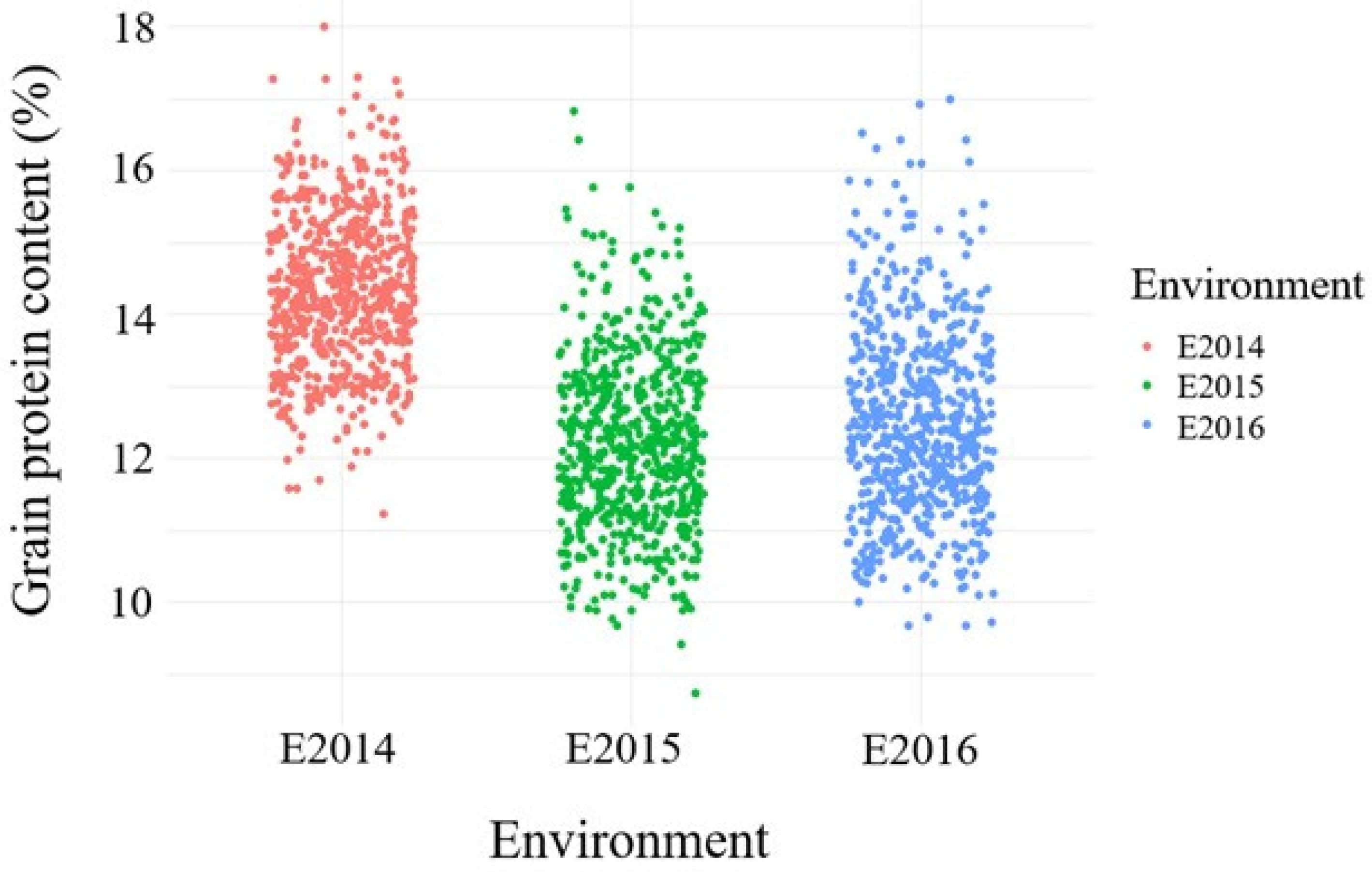
3.1. Variation of Grain Protein Content across Environments

The GPC values of the NAM650 population ranged from 11.2–18.0% in 2014, 8.7–16.8% in 2015, and 9.7–17.0% in 2016 (Figure 1), with 2014 having the highest mean GPC. A Shapiro–Wilk normality test showed that GPC was normally distributed for the three environments with a p-value > 0.05. Distributions of GPC values were normal in the three environments (Figure S1), with significant positive correlations (R2 = 0.49 for 2014 and 2015, R2 = 0.42 for 2014 and 2016, and R2 = 0.57 for 2015 and 2016). Broad-sense heritability for GPC was moderate to high, ranging between H2 = 0.62 in 2014, H 2= 0.36 in 2015, and H2 = 0.68 in 2016. The average GPC for the 26 families evaluated in this study is presented in Tables S1 and S2. Using this data, seven families totaling 175 RILs (NAM175) were selected for low variation in GPC to identify loci controlling stability of the GPC (Table S3).

3.2. Stability Analysis

Stability index (b), environmental effect (t), and genotypic effect (g) values were obtained for the NAM175 population. Absolute values of the stability index for NAM175 RILs ranged from 0.00 to 2.504 and were normally distributed. Thirty RILs were identified which had no significant difference of stability index from 0 using individual t-test (p < 0.05). Environment 2014 was observed to be the most favorable for high GPC. The NAM175 population was divided into five categories based on the GPC and stability index, the trends of which are depicted by solid lines in Figure 2. Categories 2, 3, and 5 include the stable GPC lines, with GPC in the range of 15–17%, 14–15%, and 9–14%, respectively (Figure 2). Categories 1 and 4 represent the plastic lines, with reversal of GPC when moving to other environments. Categories 1, 2, 3, 4, and 5 include 81, 15, 9, 64, and 6 RILs, respectively.

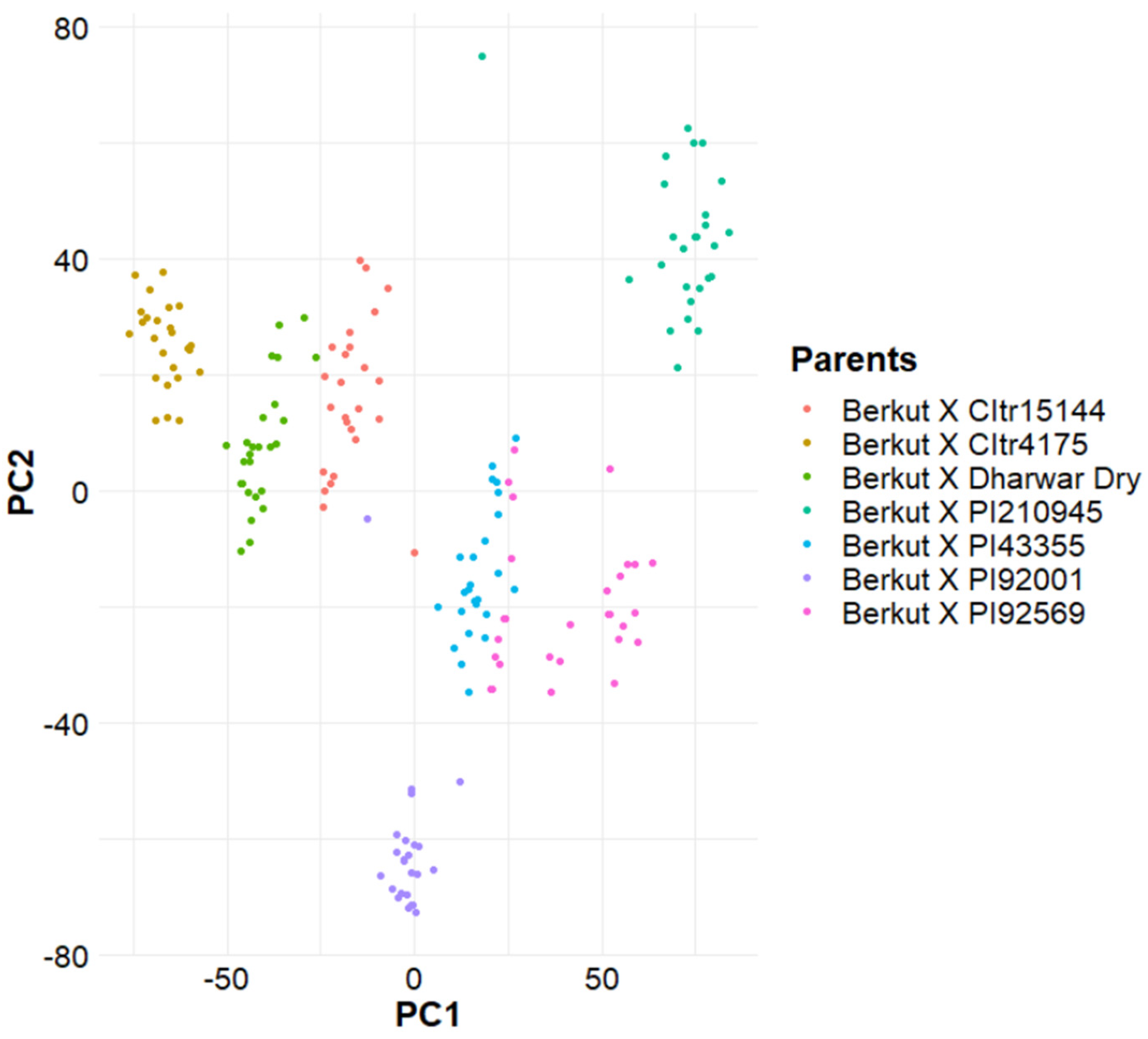
3.3. Population Structure Analysis

Population structure analyzed with PCA separated the NAM175 population into seven separate groups based on their different parents, in addition to the common parent ‘Berkut’ (Figure 3). The PC1 accounted for 7.0% of the variation, whereas the PC2 explained 5.0% of the genetic variation (Supplementary Figures S2 and S3). Kinship plots obtained from VanRaden algorithms in GAPIT also separated the population into seven different groups (data not shown). Inclusion of a different number of PCs as covariates in the GWAS model demonstrated that the first three PCs best control the false positives and false negatives, as evident from the Q–Q plots (Supplementary Figure S4), and, similarly, the model selection function based on BIC showed that first PCs should be used in the GWAS models. The Fst coefficient was 0.11 for the NAM175 and 0.18 for that NAM650, and this provided us with information about the genetic relatedness among the individuals within each population.

3.4. Marker–Trait Associations for the Stability of Grain Protein Content

Eighteen QTLs controlling GPC stability were identified with the help of four different GWAS models using a stringent Bonferroni correction of α = 0.05 (Table 1; Figure S4). The variation explained by each locus ranged from −4.19 to 3.98%. Out of these eighteen QTLs, eight were identified by two or more GWAS models simultaneously and will be referred to as high confidence QTLs (to be discussed later) (Table 1). Cumulatively, these loci explained 35.40% of the phenotypic variation. Out of those eight high confidence QTLs, three were located on chromosome 3B and chromosomes 1A, 2A, 4D, 5B, and 7D had one significant association. The QTLs on 1A, 2A, 3B, 4D, and 7D had a positive effect on increasing GPC stability, while three other OTLs had a negative effect on GPC stability. The parents of origin for associated alleles are provided in Table 1. Removal of those alleles from a breeding program by selecting for alternative alleles at these loci will favor the development of lines having increased GPC stability.
Eight significant QTLs were identified using the GPC values obtained across the environments as the response trait (Table 2; Supplementary Figures S5 and S6). Out of these eight QTLs, three were identified by two or more GWAS models simultaneously and will be referred to as high confidence QTLs (to be discussed later) (Table 2). Cumulatively, these loci explained 24.80% of the phenotypic variation. Out of those three high confidence QTLs, each of them was located on chromosomes 2B, 7A, and 7B. The QTL on 2B and 7B positively affects GPC, while the QTL on 7A negatively affected GPC such that removing those alleles would increase GPC. As there are multiple alleles with favorable effects identified from various different parental lines, pre-breeding efforts will be required to introgress all the QTLs identified. As some QTLs were identified from landraces, selection during this pre-breeding process may help reduce linkage drag.
Twelve significant QTLs were identified for grain protein content deviation obtained across the environments as the response trait (Table 3). Out of these twelve QTLs, three were identified by two or more GWAS models simultaneously and will be referred to as high confidence QTLs (to be discussed later) (Table 3). Cumulatively, these loci explained 27.63% of the phenotypic variation. Loci controlling GPC stability, GPC, and GPD are different, demonstrating separate genetic architectures for each trait which could be selected simultaneously.

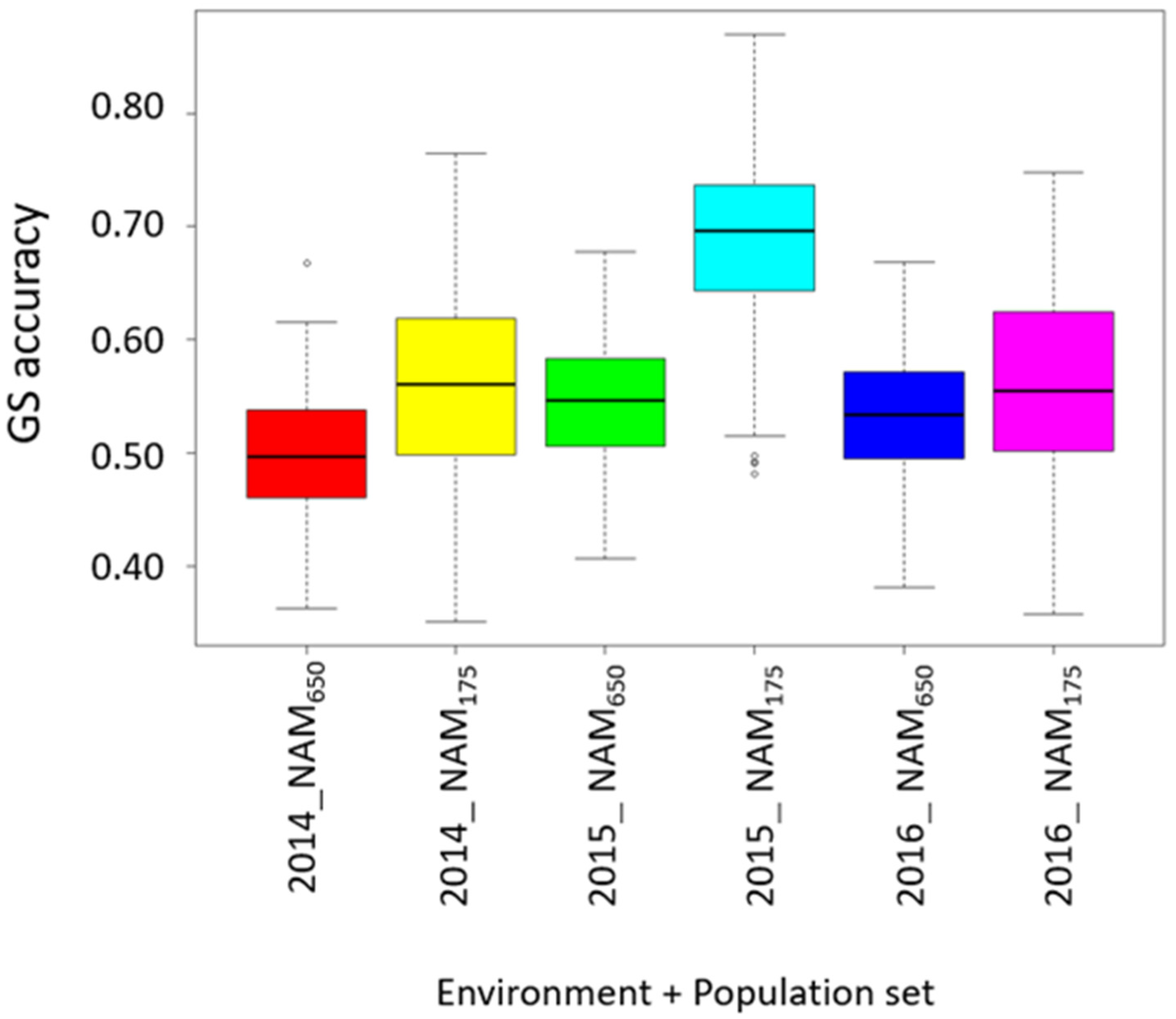
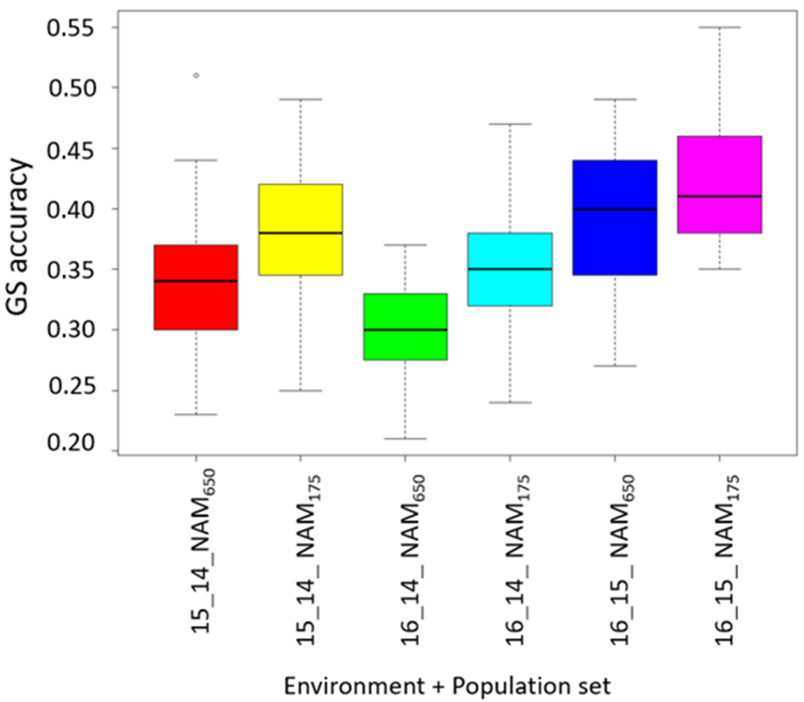
3.5. Prediction for Grain Protein Content and Stability

The prediction accuracy for GPC in the NAM650 population was r = 0.50 in 2014, r = 0.55 in 2015, and r = 0.53 in 2016. Overall, GPC stability was less predictable with prediction accuracy values between r = 0.34 and 0.44 and a mean of 0.40. There was a significant difference in prediction accuracy for GPC and GPC stability, which was assessed using Tukey’s test (p-value < 0.05; F statistics = 9.9). The prediction accuracy of GPC in the selected NAM175 subset ranged between r = 0.56 to 0.69. The maximum prediction accuracy of r = 0.69 was achieved again for the 2015 environment, while the lowest prediction accuracy of r = 0.56 was obtained for the 2014 environment. Comparison of prediction accuracies for each environment using the two different sets of populations is presented in Figure 4. Prediction accuracy is generally high when using the NAM175, increasing by 15% as compared to the NAM650.
GS accuracy was significantly lower for the independent validation of each population set and under different environments compared to cross-validation GS accuracies assessed using Tukey’s test (p-value < 0.05; F statistic = 9.2) (Figure 5). Independent prediction accuracies for the NAM650 population ranged between r = 0.30 to 0.39 and ranged between r = 0.35 to 0.43 for the NAM175 for GPC. The independent prediction accuracies were higher for the NAM175, and the same results were observed during the cross-validation prediction scenario. The highest independent prediction accuracy was obtained by a training model on 2015 GPC to 2016 GPC (Figure 5).

4. Discussion

4.1. Stability of Genotypes across Environments

A primary goal of plant breeding programs is to select germplasms with superior adaptation to the targeted environments. The performance of genotypes may range from those that are very well adapted to a narrower set of environments and perform below average in others to genotypes that perform consistently relative to others across a wider range of environments and are considered to have greater stability. Herein, we used a static stability concept, targeting a predetermined value of GPC across all the environments. There are numerous statistical tools for analyzing static stability but here we applied FW regression analysis as it is capable of summarizing the interactions in comprehensible ways [9].
Crossover and non-crossover interactions were observed in our FW regression analysis which included reversals in rank and scale effects for GPC due to environmental effects and G*E interactions. Identification of only thirty lines with stable GPC across the environments out of 650 lines highlights the challenge of maintaining an adequate population size when selecting for a complex quantitative trait in genetically diverse germplasm. Evaluating this population in a greater number of environments would provide more insight into the genetic control of this trait. Additionally, the founder parents of the NAM population are primarily landraces that have not undergone routine selection for GPC [37], as has been performed with contemporary germplasms for at least the past 60 years. The stable lines varied in their average GPC, but lines having high and stable GPC (Category 2) demonstrate the ability to select genotypes for these traits. The lines identified in this study having high GPC and stability are particularly useful for introgression into modern breeding germplasm to expand available allelic variation for this important trait.

4.2. Genomic Regions Controlling Stability of GPC

The QTLs associated with GPC stability and GPC per se performance were not detected in the same genomic regions, suggesting that GPC stability and GPC are under the control of different genes. Accounting for the different genetic architectures of these two traits could aid the indexed selection for the desired GPC along with stability. Different QTLs controlling yield stability and yield per se in wheat have similarly been documented [61]. In maize, yield and yield stability were observed to be independent, demonstrating the potential for simultaneous selection for both traits [62]. Loci controlling yield stability were located in the same regions as QTLs for yield and yield-component traits in a barley mapping effort [63]. Critical factors that are not captured or quantifiable in each of these yield-related studies are the precise abiotic or biotic factors limiting yield potential in different environments. Thus, stability is an important aspect to consider, and our study suggests that breeding programs may select for both GPC and GPC stability by treating them as separate traits for developing varieties grown in climates with environmental variables that are difficult to predict.
Genomic regions controlling GPC stability have not been investigated in wheat based on the available literature. In the present study, eight high confidence QTLs controlling GPC stability distributed over six chromosomes were identified that individually explained −4.19 to 3.98% of variation for GPC stability. The QTLs on 1A, 2A, 3B, 4D, and 7D had a positive effect on GPC stability, while three other OTLs had a negative effect on GPC stability. Similar results were obtained by Sehgal et al. when mapping genomic regions for yield stability, where 11 QTLs associated with yield stability were distributed on seven chromosomes [64]. The amount of phenotypic variation explained by their yield stability QTLs varied from 3.2 to 8.1%. Thus, although stability is an important consideration when selecting for complex quantitative traits, such as yield and GPC, appropriate index weighting in genomic selection approaches is most likely an improved alternative in selection schemes.
Marker–trait associations have reported QTLs for GPC on all 21 chromosomes of wheat [65,66,67,68,69]. Loci controlling GPC were mapped to chromosomes 1A, 2B, 3B, 4A, 6B, 7A, and 7B in this study. The region linked to SpringWheatNAM_tag_190170 on 1A was previously identified in a DH population using composite interval mapping [70] and Groos et al. [66] used an F7 RIL population grown in five environments. The favorable allele for this locus was identified in Berkut and Dharwar Dry, both of which are modern cultivars. The 7A GPC locus was discovered in the same region as another investigation [70,71]. These studies also reported that this locus had a negative effect on total GPC. Loci on chromosomes 3B and 4A have not been previously reported for GPC in wheat [14,67,72], which may be due to no prior utilization of these landraces in mapping studies [37]. These two loci had a negative effect on GPC, with associated alleles identified in the landraces. The utilization of diverse landraces in this study provides information about different genomic regions that are absent in present-day cultivars [73].
Similar to GPC stability loci, QTLs controlling GPC per se explained a small portion of the variance (24.80%). Given the number of small-effect loci controlling each trait, the GS approach proposed in this study should improve the ability to select for these traits simultaneously during the breeding process. The utilization of indexed genomic selection would assist in selecting simultaneously for GPC stability and GPC [74]. Rapp et al. [71] demonstrated the use of phenotypic and genomic selection indices to select durum wheat lines for high GPC and grain yield. Similarly, lines having high GPC and grain yield were selected using index selection in a multi-variate GS model for wheat [75]. These studies suggested that utilization of index selection in multi-variate GS models would potentially aid in selecting lines having stable GPC in addition to high GPC and grain yield.

4.3. Accuracy for Predicting GPC and GPC Stability

Prediction accuracy for GPC ranged between 0.50 and 0.69, which is moderately higher than prediction accuracies for grain yield [38,39]. Heritability of GPC, the effect of the NAM population, and population sizes used for training the GS models would each affect prediction accuracy [76,77]. Our results are consistent with previous studies where high heritability has resulted in better prediction accuracies in cereals [78]. The heritability of GPC is usually higher than yield, which ultimately resulted in better predictions for GPC [79]. In a genomic prediction experiment for grain yield in oats (Avena sativa L.), lower prediction accuracy was obtained because the experiment was planted under diverse environmental conditions, resulting in reduced genetic variance as compared to G*E interactions and thereby reduced heritability [80]. The NAM population in the current study was investigated in more homogenous target environments for wheat production in the PNW. This should result in a relatively lower G*E variance relative to genetic variance, leading to a higher heritability estimate and an increase in genomic selection accuracy.
Prior studies are not available to compare the accuracy of GS for GPC stability with stability index values obtained from FW regression in wheat. GS accuracies for GPC stability were significantly (p < 0.05) lower than GPC, suggesting a more complex architecture for GPC stability. Huang et al. [36] conducted GS for grain yield, test weight, and flour protein content stability using an additive main effect and multiplicative interaction (AMMI) model in wheat. They observed an accuracy from 0.14 to 0.31 for the stability of flour protein using four different GS models, namely, Bayesian ridge regression (0.14), elastic net (0.27), rrBLUP (0.31), and RKHS (0.31). Their study also demonstrated that the stability index for quality traits has less prediction accuracy than the trait itself. Our results, coupled with those of Huang et al. [36], suggest that GS can be used for predicting GPC stability. Furthermore, the prediction accuracy for GPC stability could be improved by obtaining a stability index from a larger number of field trials, as a large number of environments are useful for more reliable estimations of stability [81]. The GS models could be retrained by incorporating data from additional environments in subsequent years. High prediction accuracies for stability could better predict the performance of genotypes at multiple locations during breeding cycles [82].
There was an improvement of prediction accuracy when the model was trained on NAM175 compared to the NAM650 population. This is in contrast to other studies where it was observed that prediction accuracies improve when the number of individuals in the training population increases [83,84,85]. This argument was strengthened by the population differentiation coefficient (Fst), suggesting that lines in the NAM175 were more genetically related compared to the NAM650. It has been observed that prediction accuracies increase when training and testing populations are more genetically related to each other, as was the case in the NAM175 population set [86,87]. These results suggest that selection for lines having GPC stability also aids in the improvement of GS accuracy for GPC. This study opens up an avenue for the utilization of GS in a spring wheat breeding program selecting lines having GPC stability in addition to high GPC.

5. Conclusions

Selection for GPC is often secondary to grain yield in terms of breeding objectives for spring wheat, although it is a primary trait that producers consider when selecting varieties. We report the first large-scale study of nested association mapping and evaluation of GS for GPC stability in wheat. This study identified wheat lines having less variation for GPC and mapped QTLs controlling GPC stability, an important and often overlooked trait. The identification of stable genotypes with high GPC could help in developing cultivars that can perform similarly in multiple environments. The QTLs identified in this study explained a small amount of phenotypic variation, demonstrating the complexity of the trait, which suggests a GS approach could best address breeding for GPC and GPC stability. Prediction accuracy is sufficiently high for the implementation of GS for GPC and GPC stability in this study. With the implementation of GS for these traits, predictions can be available while evaluating grain yield, enabling selection for GPC along with agronomic and yield traits.

Supplementary Materials

The following are available online at https://www.mdpi.com/article/10.3390/agronomy11122528/s1. Supplementary Table S1: Average grain protein content of 26 NAM families across the three environments planted at Spillman Agronomy Farm, Pullman, WA; Supplementary Table S2. Phenotypic description and broad sense heritability of the grain protein content across the three environments (2014-16); Supplementary Table S3: Average grain protein content and standard deviation for families selected to have less variation. The origin represents countries of the NAM population founder parents; Supplementary Figure S1: Distribution of average GPC for environments 2014, 2015, and 2016. The X-axis shows the environments, namely, 2014, 2015, and 2016, the Y-axis shows the density of individuals; Supplementary Figure S2: Variation explained in the NAM175 population by each principal component obtained in this study; Supplementary Figure S3: Population structure inferred from principal component analysis and illustrated with the first three principal component’s; Supplementary Figure S4: Manhattan plot representing the position of significant markers controlling the grain protein content stability. The threshold used for the significant association is a Bonferroni correction of 0.05 (A). Quantile-Quantile (Q-Q) plot of marker-trait association study using different principal components as a covariate in the BLINK model for grain protein content stability (B); Supplementary Figure S5: Manhattan plot representing the position of significant markers controlling the grain protein content. The threshold used for significant association is a Bonferroni correction of 0.05 (A). Quantile-Quantile (Q-Q) plot of marker-trait association study using different principal components as a covariate in the BLINK model for grain protein content (B); Supplementary Figure S6: Linkage disequilibrium analysis on the population using complete set of the marker data.

Author Contributions

Conceptualization: K.S.S., P.D.M. and A.H.C.; data analysis: K.S.S. and P.D.M.; writing—original draft preparation: K.S.S.; writing—review and editing: P.D.M., M.J.L., M.O.P. and A.H.C.; supervision: M.O.P. and A.H.C.; project administration: M.O.P. and A.H.C.; funding acquisition: M.O.P. and A.H.C. All authors have read and agreed to the published version of the manuscript.

Funding

This project was supported by the Agriculture and Food Research Initiative Competitive Grant 2017-67007-25939 (WheatCAP) and 2016-68004-24770 from the USDA National Institute of Food and Agriculture and Hatch project 1014919.

Conflicts of Interest

The authors declare no conflict of interest.

References

  1. Shewry, P.R.; Halford, N.G. Cereal seed storage proteins: Structures, properties and role in grain utilization. J. Exp. Bot. 2002, 53, 947–958. [Google Scholar] [CrossRef] [Green Version]
  2. Shewry, P.R. Improving the protein content and composition of cereal grain. J. Cereal Sci. 2007, 46, 239–250. [Google Scholar] [CrossRef]
  3. Vogel, K.P.; Johnson, V.A.; Mattern, P.J. Protein and Lysine Content of Grain, Endosperm, and Bran of Wheats from the USDA World Wheat Collection. Crop Sci. 1976, 16, 655–660. [Google Scholar] [CrossRef] [Green Version]
  4. Löffler, C.M.; Busch, R.H. Selection for Grain Protein, Grain Yield, and Nitrogen Partitioning Efficiency in Hard Red Spring Wheat. Crop Sci. 1982, 22, 591–595. [Google Scholar] [CrossRef]
  5. DePauw, R.M.; Knox, R.E.; Clarke, F.R.; Wang, H.; Fernandez, M.R.; Clarke, J.M.; McCaig, T.N. Shifting undesirable correlations. In Proceedings of the Euphytica. Euphytica 2007, 157, 409–415. [Google Scholar] [CrossRef]
  6. De Kroon, H.; Huber, H.; Stuefer, J.F.; Van Gorenendael, J.M. A modular concept of phenotypic plasticity in plants. New Phytol. 2005, 166, 73–82. [Google Scholar] [CrossRef] [PubMed]
  7. Kusmec, A.; Srinivasan, S.; Nettleton, D.; Schnable, P.S. Distinct genetic architectures for phenotype means and plasticities in Zea mays. Nat. Plants 2017, 3, 715–723. [Google Scholar] [CrossRef] [PubMed]
  8. Kliebenstein, D.J.; Figuth, A.; Mitchell-olds, T. Genetic Architecture of Plastic Methyl Jasmonate Responses in Arabidopsis thaliana. Genetics 2002, 1696, 1685–1696. [Google Scholar] [CrossRef] [PubMed]
  9. Eberhart, S.A.; Russell, W.A. Stability Parameters for Comparing Varieties. Crop Sci. 1966, 6, 36–40. [Google Scholar] [CrossRef] [Green Version]
  10. Lin, C.S.; Binns, M.R.; Lefkovitch, L.P. Stability Analysis: Where Do We Stand? Crop Sci. 1986, 26, 894–900. [Google Scholar] [CrossRef] [Green Version]
  11. Finlay, K.W.; Wilkinson, G.N. The analysis of adaptation in a plant-breeding programme. Aust. J. Agric. Res. 1963, 14, 742–754. [Google Scholar] [CrossRef] [Green Version]
  12. Lian, L.; de los Campos, G. GENOMIC SELECTION FW: An R Package for Finlay—Wilkinson Regression that Incorporates Genomic/Pedigree Information and Covariance Structures Between Environments. G3 Genes Genomes Genet. 2016, 6, 589–597. [Google Scholar] [CrossRef] [Green Version]
  13. Ordas, B.; Malvar, R.A.; Hill, W.G. Genetic variation and quantitative trait loci associated with developmental stability and the environmental correlation between traits in maize. Genet. Res. (Camb) 2008, 90, 385–395. [Google Scholar] [CrossRef] [Green Version]
  14. Blanco, A.; De Giovanni, C.; Laddomada, B.; Sciancalepore, A.; Simeone, R.; Devos, K.M.; Gale, M.D. Quantitative trait loci influencing grain protein content in tetraploid wheats. Plant Breed. 1996, 115, 310–316. [Google Scholar] [CrossRef]
  15. Huang, X.; Wei, X.; Sang, T.; Zhao, Q.; Feng, Q.; Zhao, Y.; Li, C.; Zhu, C.; Lu, T.; Zhang, Z.; et al. Genome-wide asociation studies of 14 agronomic traits in rice landraces. Nat. Genet. 2010, 42, 961–967. [Google Scholar] [CrossRef]
  16. Zhu, C.; Gore, M.; Buckler, E.S.; Yu, J. Status and Prospects of Association Mapping in Plants. Plant Genome J. 2008, 1, 5–20. [Google Scholar] [CrossRef]
  17. Kaur, B.; Sandhu, K.S.; Kamal, R.; Kaur, K.; Singh, J.; Röder, M.S.; Muqaddasi, Q.H. Omics for the Improvement of Abiotic, Biotic, and Agronomic Traits in Major Cereal Crops: Applications, Challenges, and Prospects. Plants 2021, 10, 1989. [Google Scholar] [CrossRef]
  18. Yu, J.; Buckler, E.S. Genetic association mapping and genome organization of maize. Curr. Opin. Biotechnol. 2006, 17, 155–160. [Google Scholar] [CrossRef]
  19. Saade, S.; Maurer, A.; Shahid, M.; Oakey, H.; Schmöckel, S.M.; Negrão, S.; Pillen, K.; Tester, M. Yield-related salinity tolerance traits identified in a nested association mapping (NAM) population of wild barley. Sci. Rep. 2016, 6, 32586. [Google Scholar] [CrossRef] [PubMed] [Green Version]
  20. Gage, J.L.; Monier, B.; Giri, A.; Buckler, E.S. Ten years of the maize nested association mapping population: Impact, limitations, and future directions. Plant Cell 2020, 32, 2083–2093. [Google Scholar] [CrossRef] [PubMed]
  21. Fragoso, C.A.; Moreno, M.; Wang, Z.; Heffelfinger, C.; Arbelaez, L.J.; Aguirre, J.A.; Franco, N.; Romero, L.E.; Labadie, K.; Zhao, H.; et al. Genetic architecture of a rice nested association mapping population. G3 Genes Genomes Genet. 2017, 7, 1913–1926. [Google Scholar] [CrossRef] [PubMed] [Green Version]
  22. Li, H.; Bradbury, P.; Ersoz, E.; Buckler, E.S.; Wang, J. Joint QTL linkage mapping for multiple-cross mating design sharing one common parent. PLoS ONE 2011, 6, e0017573. [Google Scholar] [CrossRef] [Green Version]
  23. Blanc, G.; Charcosset, A.; Mangin, B.; Gallais, A.; Moreau, L. Connected populations for detecting quantitative trait loci and testing for epistasis: An application in maize. Theor. Appl. Genet. 2006, 113, 206–224. [Google Scholar] [CrossRef]
  24. Samantara, K.; Shiv, A.; de Sousa, L.L.; Sandhu, K.S.; Priyadarshini, P.; Mohapatra, S.R. A Comprehensive Review on Epigenetic Mechanisms and Application of Epigenetic Modifications for Crop Improvement. Environ. Exp. Bot. 2021, 188, 104479. [Google Scholar] [CrossRef]
  25. Mcmullen, M.D.; Kresovich, S.; Villeda, H.S.; Bradbury, P.; Li, H.; Sun, Q.; Flint-Garcia, S.; Thornsberry, J.; Acharya, C.; Bottoms, C.; et al. Genetic Properties of the Maize Nested Association Mapping Population. Science 2009, 325, 737–740. [Google Scholar] [CrossRef] [Green Version]
  26. Würschum, T.; Liu, W.; Gowda, M.; Maurer, H.P.; Fischer, S.; Schechert, A.; Reif, J.C. Comparison of biometrical models for joint linkage association mapping. Heredity (Edinb) 2012, 108, 332–340. [Google Scholar] [CrossRef] [PubMed] [Green Version]
  27. Tian, F.; Bradbury, P.J.; Brown, P.J.; Hung, H.; Sun, Q.; Flint-garcia, S.; Rocheford, T.R.; Mcmullen, M.D.; Holland, J.B.; Buckler, E.S. Genome-wide association study of leaf architecture in the maize nested association mapping population. Nat. Genet. 2011, 43, 159–162. [Google Scholar] [CrossRef] [PubMed]
  28. Korte, A.; Ashley, F. The advantages and limitations of trait analysis with GWAS: A review. Plant Methods 2013, 9, 29. [Google Scholar] [CrossRef] [Green Version]
  29. Meuwissen, T.H.E.; Hayes, B.J.; Goddard, M.E. Prediction of Total Genetic Value Using Genome-Wide Dense Marker Maps. Genetics 2001, 157, 1819–1829. [Google Scholar] [CrossRef] [PubMed]
  30. Crossa, J.; Pérez, P.; Hickey, J.; Burgueño, J.; Ornella, L.; Cerón-Rojas, J.; Zhang, X.; Dreisigacker, S.; Babu, R.; Li, Y.; et al. Genomic prediction in CIMMYT maize and wheat breeding programs. Heredity (Edinb) 2014, 112, 48–60. [Google Scholar] [CrossRef] [PubMed] [Green Version]
  31. Robertsen, C.D.; Hjortshøj, R.L.; Janss, L.L. Genomic Selection in Cereal Breeding. Agronomy 2019, 9, 95. [Google Scholar] [CrossRef] [Green Version]
  32. Larkin, D.L.; Lozada, D.N.; Mason, R.E. Genomic Selection—Considerations for Successful Implementation in Wheat Breeding Programs. Agronomy 2019, 9, 479. [Google Scholar] [CrossRef] [Green Version]
  33. Sandhu, K.S.; Mihalyov, P.D.; Lewien, M.J.; Pumphrey, M.O.; Carter, A.H. Combining Genomic and Phenomic Information for Predicting Grain Protein Content and Grain Yield in Spring Wheat. Front. Plant Sci. 2021, 12, 170. [Google Scholar] [CrossRef]
  34. Rutkoski, J.E.; Heffner, E.L.; Sorrells, M.E. Genomic selection for durable stem rust resistance in wheat. Euphytica 2011, 179, 161–173. [Google Scholar] [CrossRef]
  35. Heffner, E.L.; Jannink, J.-L.; Iwata, H.; Souza, E.; Sorrells, M.E. Genomic Selection Accuracy for Grain Quality Traits in Biparental Wheat Populations. Crop Sci. 2011, 51, 2597–2606. [Google Scholar] [CrossRef] [Green Version]
  36. Huang, M.; Cabrera, A.; Hoffstetter, A.; Griffey, C.; Van Sanford, D.; Costa, J.; McKendry, A.; Chao, S.; Sneller, C. Genomic selection for wheat traits and trait stability. Theor. Appl. Genet. 2016, 129, 1697–1710. [Google Scholar] [CrossRef]
  37. Blake, N.K.; Pumphrey, M.; Glover, K.; Chao, S.; Jordan, K.; Jannick, J.L.; Akhunov, E.A.; Dubcovsky, J.; Bockelman, H.; Talbert, L.E. Registration of the triticeae-cap spring wheat nested association mapping population. J. Plant Regist. 2019, 13, 294–297. [Google Scholar] [CrossRef] [Green Version]
  38. Sandhu, K.; Patil, S.S.; Pumphrey, M.; Carter, A. Multitrait machine- and deep-learning models for genomic selection using spectral information in a wheat breeding program. Plant Genome 2021, e20119. [Google Scholar] [CrossRef] [PubMed]
  39. Sandhu, K.S.; Lozada, D.N.; Zhang, Z.; Pumphrey, M.O.; Carter, A.H. Deep Learning for Predicting Complex Traits in Spring Wheat Breeding Program. Front. Plant Sci. 2021, 11, 613325. [Google Scholar] [CrossRef] [PubMed]
  40. Jordan, K.W.; Wang, S.; He, F.; Chao, S.; Lun, Y.; Paux, E.; Sourdille, P.; Sherman, J.; Akhunova, A.; Blake, N.K.; et al. The genetic architecture of genome-wide recombination rate variation in allopolyploid wheat revealed by nested association mapping. Plant J. 2018, 95, 1039–1054. [Google Scholar] [CrossRef] [PubMed] [Green Version]
  41. Lanning, S.P.; Talbert, L.E.; McGuire, C.F.; Bowman, H.F.; Carlson, G.R.; Jackson, G.D.; Eckhoff, J.L.; Kushnak, G.D.; Stougaard, R.N.; Stallknecht, G.F.; et al. Registration of ‘McNeal’ Wheat. Crop Sci. 1994, 34, 1126. [Google Scholar] [CrossRef]
  42. Delwiche, S.R. Single Wheat Kernel Analysis by Near-Infrared Transmittance: Protein Content. 1995. Available online: https://www.cerealsgrains.org/publications/cc/backissues/1995/Documents/72_11.pdf (accessed on 23 November 2021).
  43. Delwiche, S.R. Protein Content of Single Kernels of Wheat by Near-Infrared Reflectance Spectroscopy. J. Cereal Sci. 1998, 27, 241–254. [Google Scholar] [CrossRef]
  44. Olmos, S.; Distelfeld, A.; Chicaiza, O.; Schlatter, A.R.; Fahima, T.; Echenique, V.; Dubcovsky, J. Precise mapping of a locus affecting grain protein content in durum wheat. Theor. Appl. Genet. 2003, 107, 1243–1251. [Google Scholar] [CrossRef] [Green Version]
  45. Distelfeld, A.; Uauy, C.; Fahima, T.; Dubcovsky, J. Physical map of the wheat high-grain protein content gene Gpc-B1 and development of a high-throughput molecular marker. New Phytol. 2006, 169, 753–763. [Google Scholar] [CrossRef] [PubMed] [Green Version]
  46. R Development Core Team. R: A Language and Environment for Statistical Computing; R Foundation for Statistical Computing: Vienna, Austria, 2020; p. 201. ISBN 978-0792305866. [Google Scholar]
  47. Rodríguez, F.; Alvarado, G.; Pacheco, Á.; Burgueno, J. ACBD-R. Augmented Complete Block Design with R for Windows. Version 4.0. CIMMYT Res. Data Softw. Repos. Netw. 2018. [Google Scholar]
  48. Monaghan, J.M.; Snape, J.W.; Chojecki, A.J.S.; Kettlewell, P.S. The use of grain protein deviation for identifying wheat cultivars with high grain protein concentration and yield. Euphytica 2001, 122, 309–317. [Google Scholar] [CrossRef]
  49. Mosleth, E.F.; Lillehammer, M.; Pellny, T.K.; Wood, A.J.; Riche, A.B.; Hussain, A.; Griffiths, S.; Hawkesford, M.J.; Shewry, P.R. Genetic variation and heritability of grain protein deviation in European wheat genotypes. Field Crops. Res. 2020, 255, 107896. [Google Scholar] [CrossRef]
  50. Marcussen, T.; Sandve, S.R.; Heier, L.; Pfeifer, M.; Kugler, K.G.; Sandve, S.R.; Zhan, B. A chromosome-based draft sequence of the hexaploid bread wheat (Triticum aestivum) genome Ancient hybridizations among the ancestral genomes of bread wheat Genome interplay in the grain transcriptome of hexaploid bread wheat Structural and functional pa. Science 2014, 345, 6194. [Google Scholar]
  51. Lipka, A.E.; Tian, F.; Wang, Q.; Peiffer, J.; Li, M.; Bradbury, P.J.; Gore, M.A.; Buckler, E.S.; Zhang, Z. GAPIT: Genome association and prediction integrated tool. Bioinformatics 2012, 28, 2397–2399. [Google Scholar] [CrossRef] [Green Version]
  52. Vanraden, P.M. Efficient Methods to Compute Genomic Predictions. J. Dairy Sci. 2008, 91, 4414–4423. [Google Scholar] [CrossRef] [Green Version]
  53. Price, A.L.; Patterson, N.J.; Plenge, R.M.; Weinblatt, M.E.; Shadick, N.A.; Reich, D. Principal components analysis corrects for stratification in genome-wide association studies. Nat. Genet. 2006, 38, 904–909. [Google Scholar] [CrossRef] [PubMed]
  54. SAS Institute Inc. SAS® 9.3 System Options: Reference; SAS Institute Inc.: Cary, NC, USA, 2011. [Google Scholar]
  55. Yu, J.; Pressoir, G.; Briggs, W.H.; Bi, I.V.; Yamasaki, M.; Doebley, J.F.; McMullen, M.D.; Gaut, B.S.; Nielsen, D.M.; Holland, J.B.; et al. A unified mixed-model method for association mapping that accounts for multiple levels of relatedness. Nat. Genet. 2006, 38, 203–208. [Google Scholar] [CrossRef] [PubMed]
  56. Zhang, Z.; Ersoz, E.; Lai, C.; Todhunter, R.J.; Tiwari, H.K.; Gore, M.A.; Bradbury, P.J.; Yu, J.; Arnett, D.K.; Ordovas, J.M.; et al. Mixed linear model approach adapted for genome-wide association studies. Nat. Genet. 2010, 42, 355–360. [Google Scholar] [CrossRef] [Green Version]
  57. Liu, X.; Huang, M.; Fan, B.; Buckler, E.S.; Zhang, Z. Iterative Usage of Fixed and Random Effect Models for Powerful and Efficient Genome-Wide Association Studies. PLoS Genet. 2016, 12, e1005767. [Google Scholar] [CrossRef] [PubMed]
  58. Huang, M.; Liu, X.; Zhou, Y.; Summers, R.M.; Zhang, Z. BLINK: A package for the next level of genome-wide association studies with both individuals and markers in the millions. Gigascience 2018, 8, 1–12. [Google Scholar] [CrossRef]
  59. Holm, S. A Simple Sequentially Rejective Multiple Test Procedure. Scand. J. Stat. 1978, 6, 65–70. [Google Scholar]
  60. Endelman, J.B. Ridge Regression and Other Kernels for Genomic Selection with R Package rrBLUP. Plant Genome 2011, 4, 250–255. [Google Scholar] [CrossRef] [Green Version]
  61. Berke, T.G.; Baenziger, P.S.; Morris, R. Chromosomal location of wheat quantitative trait loci affecting agronomic performance of seven traits, using reciprocal chromosome substitutions. Crop Sci. 1992, 32, 621–627. [Google Scholar] [CrossRef]
  62. Tollenaar, M.; Lee, E.A. Yield potential, yield stability and stress tolerance in maize. Field Crops Res. 2002, 75, 161–169. [Google Scholar] [CrossRef]
  63. Kraakman, A.T.W.; Niks, R.E.; Van Den Berg, P.M.M.M.; Stam, P.; Van Eeuwijk, F.A. Linkage disequilibrium mapping of yield and yield stability in modern spring barley cultivars. Genetics 2004, 168, 435–446. [Google Scholar] [CrossRef] [Green Version]
  64. Sehgal, D.; Autrique, E.; Singh, R.; Ellis, M.; Singh, S.; Dreisigacker, S. Identification of genomic regions for grain yield and yield stability and their epistatic interactions. Sci. Rep. 2017, 7, 1–12. [Google Scholar] [CrossRef] [Green Version]
  65. Blanco, A.; Simeone, R.; Gadaleta, A. Detection of QTLs for grain protein content in durum wheat. Theor. Appl. Genet. 2006, 112, 1195–1204. [Google Scholar] [CrossRef]
  66. Groos, C.; Robert, N.; Bervas, E.; Charmet, G. Genetic analysis of grain protein-content, grain yield and thousand-kernel weight in bread wheat. Theor. Appl. Genet. 2003, 106, 1032–1040. [Google Scholar] [CrossRef] [PubMed]
  67. Joppa, L.R.; Hareland, G.A.; Du, C.; Hart, G.E. Mapping gene(s) for grain protein in tetraploid wheat (Triticum turgidum L.) using a population of recombinant inbred chromosome lines. Crop Sci. 1997, 37, 1586–1589. [Google Scholar] [CrossRef]
  68. Perretant, M.R.; Cadalen, T.; Charmet, G.; Sourdille, P.; Nicolas, P.; Boeuf, C.; Tixier, M.H.; Branlard, G.; Bernard, S.; Bernard, M. QTL analysis of bread-making quality in wheat using a doubled haploid population. Theor. Appl. Genet. 2000, 100, 1167–1175. [Google Scholar] [CrossRef]
  69. Prasad, M.; Kumar, N.; Kulwal, P.L.; Röder, M.S.; Balyan, H.S.; Dhaliwal, H.S.; Gupta, P.K. QTL analysis for grain protein content using SSR markers and validation studies using NILs in bread wheat. Theor. Appl. Genet. 2003, 106, 659–667. [Google Scholar] [CrossRef]
  70. Mahjourimajd, S.; Taylor, J.; Rengel, Z.; Khabaz-Saberi, H.; Kuchel, H.; Okamoto, M.; Langridge, P. The genetic control of grain protein content under variable nitrogen supply in an Australian wheat mapping population. PLoS ONE 2016, 11, e0159371. [Google Scholar] [CrossRef] [Green Version]
  71. Rapp, M.; Lein, V.; Lacoudre, F.; Lafferty, J.; Müller, E.; Vida, G.; Bozhanova, V.; Ibraliu, A.; Thorwarth, P.; Piepho, H.P.; et al. Simultaneous improvement of grain yield and protein content in durum wheat by different phenotypic indices and genomic selection. Theor. Appl. Genet. 2018, 131, 1315–1329. [Google Scholar] [CrossRef]
  72. Heo, H.; Sherman, J. Identification of QTL for Grain Protein Content and Grain Hardness from Winter Wheat for Genetic Improvement of Spring Wheat. Plant Breed. Biotechnol. 2013, 1, 347–353. [Google Scholar] [CrossRef] [Green Version]
  73. He, F.; Pasam, R.; Shi, F.; Kant, S.; Keeble-Gagnere, G.; Kay, P.; Forrest, K.; Fritz, A.; Hucl, P.; Wiebe, K.; et al. Exome sequencing highlights the role of wild-relative introgression in shaping the adaptive landscape of the wheat genome. Nat. Genet. 2019, 51, 896–904. [Google Scholar] [CrossRef]
  74. Schulthess, A.W.; Wang, Y.; Miedaner, T.; Wilde, P.; Reif, J.C.; Zhao, Y. Multiple-trait- and selection indices-genomic predictions for grain yield and protein content in rye for feeding purposes. Theor. Appl. Genet. 2016, 129, 273–287. [Google Scholar] [CrossRef] [PubMed]
  75. Michel, S.; Löschenberger, F.; Ametz, C.; Pachler, B.; Sparry, E.; Bürstmayr, H. Simultaneous selection for grain yield and protein content in genomics-assisted wheat breeding. Theor. Appl. Genet. 2019, 132, 1745–1760. [Google Scholar] [CrossRef]
  76. Heffner, E.L.; Jannink, J.; Sorrells, M.E. Genomic Selection Accuracy using Multifamily Prediction Models in a Wheat Breeding Program. Plant Genome 2011, 4, 65–75. [Google Scholar] [CrossRef] [Green Version]
  77. Poland, J.; Endelman, J.; Dawson, J.; Rutkoski, J.; Wu, S.; Manes, Y.; Dreisigacker, S.; Crossa, J.; Sánchez-Villeda, H.; Sorrells, M.; et al. Genomic Selection in Wheat Breeding using Genotyping-by-Sequencing. Plant Genome J. 2012, 5, 103–113. [Google Scholar] [CrossRef] [Green Version]
  78. Windhausen, V.S.; Atlin, G.N.; Hickey, J.M.; Crossa, J.; Jannink, J.-L.; Sorrells, M.E.; Raman, B.; Cairns, J.E.; Tarekegne, A.; Semagn, K.; et al. Effectiveness of Genomic Prediction of Maize Hybrid Performance in Different Breeding Populations and Environments. G3 Genes Genomes Genet. 2012, 2, 1427–1436. [Google Scholar] [CrossRef] [PubMed] [Green Version]
  79. Battenfield, S.D.; Guzmán, C.; Chris Gaynor, R.; Singh, R.P.; Peña, R.J.; Dreisigacker, S.; Fritz, A.K.; Poland, J.A. Genomic selection for processing and end-use quality traits in the CIMMYT spring bread wheat breeding program. Plant Genome 2016, 9. [Google Scholar] [CrossRef] [PubMed] [Green Version]
  80. Asoro, F.G.; Newell, M.A.; Beavis, W.D.; Scott, M.P.; Jannink, J. Accuracy and Training Population Design for Genomic Selection on Quantitative Traits in Elite North American Oats. Plant Genome 2011, 4, 132–144. [Google Scholar] [CrossRef] [Green Version]
  81. Piepho, H.-P. Methods for Comparing the Yield Stability of Cropping Systems. J. Agron. Crop Sci. 1998, 180, 193–213. [Google Scholar] [CrossRef]
  82. Sandhu, K.S.; Aoun, M.; Morris, C.F.; Carter, A.H. Genomic Selection for End-Use Quality and Processing Traits in Soft White Winter Wheat Breeding Program with Machine and Deep Learning Models. Biology 2021, 10, 689. [Google Scholar] [CrossRef]
  83. Isidro, J.; Jannink, J.L.; Akdemir, D.; Poland, J.; Heslot, N.; Sorrells, M.E. Training set optimization under population structure in genomic selection. Theor. Appl. Genet. 2015, 128, 145–158. [Google Scholar] [CrossRef] [Green Version]
  84. Lorenz, A.J.; Chao, S.; Asoro, F.G.; Heffner, E.L.; Hayashi, T.; Iwata, H.; Smith, K.P.; Sorrells, M.E.; Jannink, J. Genomic Selection in Plant Breeding: Knowledge and Prospects. Adv. Agron. 2011, 110, 77–123. [Google Scholar]
  85. Lorenzana, R.E.; Bernardo, R. Accuracy of genotypic value predictions for marker-based selection in biparental plant populations. Theor. Appl. Genet. 2009, 120, 151–161. [Google Scholar] [CrossRef] [PubMed]
  86. Heffner, E.L.; Lorenz, A.J.; Jannink, J.L.; Sorrells, M.E. Plant breeding with Genomic selection: Gain per unit time and cost. Crop Sci. 2010, 50, 1681–1690. [Google Scholar] [CrossRef]
  87. Lorenz, A.J.; Smith, K.P. Adding genetically distant individuals to training populations reduces genomic prediction accuracy in Barley. Crop Sci. 2015, 55, 2657–2667. [Google Scholar] [CrossRef] [Green Version]
Figure 1. Variation of grain protein content for all the NAM650 across the three environments. The X-axis depicts the three environments, namely 2014, 2015, and 2016; the Y-axis shows the GPC as a percentage.
Agronomy 11 02528 g001
Figure 2. Trends for the stability index and GPC observed in the NAM175 population. The slopes of the lines represent the stability index, the X-axis depicts the environmental effect, and the Y-axis shows the grain protein content.
Agronomy 11 02528 g002
Figure 3. Population structure inferred from principal component analysis and illustrated with the first two principal components’ help. The whole population is subgrouped into seven groups, each group representing a single NAM family. Different colors in the figure represents the seven different NAM families evaluated in this study for grain protein content stability.
Agronomy 11 02528 g003
Figure 4. Comparison of GS prediction accuracies for the NAM650 and NAM175 populations for GPC. The X-axis represents the combination of population and environment, and the Y-axis represents the prediction accuracies.
Agronomy 11 02528 g004
Figure 5. Comparison of independent prediction accuracies for the NAM650 and NAM175 populations for GPC. The X-axis represents the combination of population and environment, the first number representing the testing environment while the second number represents the environment on which the GS model was trained; the Y-axis represents the prediction accuracies.
Agronomy 11 02528 g005
Table 1. Significant markers representing quantitative trait loci for grain protein content stability in a nested association mapping of hard spring wheat identified using four different GWAS models.
Marker Description Allelic Effect Significance Values
SNP nameChromosomePosition on ChromosomeAlleles Parental Line with Bolded AlleleModel Providing Significant ResultsMinor Allele FrequencyCumulative R2p-Value (Bonf.)
SpringWheatNAM_tag_81337:591A50917564C/TBerkut, Dharwar DryBLINK, MLM, CMLM0.40+1.157.91 × 10−8
SpringWheatNAM_tag_3027181B381359110A/GCItr15144BLINK0.12−4.191.32 × 10−7
SpringWheatNAM_tag_948532A569963539T/GCItr15144, PI210945, PI92001, Dharwar DryBLINK, MLM, CMLM0.36+3.681.06 × 10−6
SpringWheatNAM_tag_2723132A196126844C/GBerkut, Dharwar DryFarmCPU0.15+1.589.39 × 10−7
SpringWheatNAM_tag_2690742B155136626A/CPI210945, PI43355BLINK0.11−3.625.67 × 10−12
BS00036168_513A6.89 × 108T/CCItr15144FarmCPU0.17−2.012.16 × 10−7
SpringWheatNAM_tag_846333B23359725A/TPI92569BLINK, MLM, CMLM0.14−3.981.05 × 10−8
SpringWheatNAM_tag_70373B508522245G/TBerkut, Dharwar Dry, PI92569BLINK, MLM, CMLM0.42−1.272.84 × 10−9
SpringWheatNAM_tag_755843B6.77 × 108T/GBerkut, CItr15144, PI210945, PI92569MLM and CMLM0.29+2.530.000218
SpringWheatNAM_tag_2811644A309647389T/CBerkut, Dharwar Dry, CItr15144, PI210945,BLINK0.30−0.512.84 × 10−9
SpringWheatNAM_tag_755844D6.77 × 108A/GCItr15144, PI210945, PI92001, Dharwar Dry, BerkutMLM and CMLM0.43+1.680.000218
SpringWheatNAM_tag_170345B4.31 × 108T/CPI210945, PI43355, PI92569MLM and CMLM0.41−0.740.000399
SpringWheatNAM_tag_18817:227B100166484C/ABerkut, Dharwar DryFarmCPU0.27+2.132.81 × 10−8
SpringWheatNAM_tag_1088397B98739595T/GCItr15144, PI210945FarmCPU0.32+1.062.43 × 10−7
SpringWheatNAM_tag_370747B720870596C/GCItr15144, PI210945, PI92001FarmCPU0.25−2.709.39 × 10−7
SpringWheatNAM_tag_720257B721085362A/CBerkut, Dharwar DryFarmCPU0.17+0.436.48 × 10−7
SpringWheatNAM_tag_373627B720892406G/TPI92569FarmCPU0.20+1.892.00 × 10−7
SpringWheatNAM_tag_2800957D57137544A/CDharwar Dry, BerkutMLM and CMLM0.15+0.250.000187
Description of markers representing the tag of SNP, allele form of the tag SNP, minor allele frequency, chromosome, and position; phenotypic variation explained by the marker polymorphism: + increasing effect of minor allele, – decreasing effect of minor allele; Minor alleles are bolded.
Table 2. Significant markers representing quantitative trait loci for grain protein content in a nested association mapping of hard spring wheat.
Marker Description Allelic Effect Significance Values
SNP NameChromosomePosition on Chromosome (cM)Alleles Parental Line with Bolded AlleleModel Providing Significant ResultsMinor Allele FrequencyCumulative R2p-Value
SpringWheatNAM_tag_1901701A1.24 × 108T/CBerkut, Dharwar DryBLINK0.49+6.781.60 × 10−8
SpringWheatNAM_tag_1278081A3.66 × 108T/ABerkut, Dharwar DryFarmCPU0.14+3.026.07 × 10−17
SpringWheatNAM_tag_823062B7.17 × 108A/TCItr4175MLM, CMLM0.16+0.444.33 × 10−5
SpringWheatNAM_tag_322643B125543693A/TBerkut, PI43355BLINK0.34−7.301.26 × 10−6
SpringWheatNAM_tag_821544A6.4 × 108C/ACItr15144, PI210945, CItr4175.BLINK0.26−2.341.23 × 10−7
SpringWheatNAM_tag_1242066B7.07 × 108A/GPI43355FarmCPU0.14−1.021.74 × 10−15
SpringWheatNAM_tag_1363227A6.67 × 108T/GBerkut, PI43355BLINK, MLM, CMLM0.41−0.321.55 × 10−8
SpringWheatNAM_tag_1223697B6.19 × 108C/GBerkut, Dharwar DryMLM, CMLM0.16+3.595.31 × 10−5
Description of markers representing the tag of SNP, allele form of the tag SNP, minor allele frequency, chromosome, and position; Phenotypic variation explained by the marker polymorphism: + increasing effect of minor allele, – decreasing effect of minor allele; Minor alleles are bolded.
Table 3. Significant markers representing quantitative trait loci for grain protein content deviation in a nested association mapping of hard spring wheat.
Marker Description Allelic Effect Significance Values
SNP NameChromosomePosition on Chromosome (cM)Model Providing Significant ResultsMinor Allele FrequencyCumulative R2p-Value
SpringWheatNAM_tag_1278081A3.66 × 108FarmCPU0.14+3.537.26 × 10−8
BS00022409_512A745092365FarmCPU0.11+2.181.06 × 10−10
SpringWheatNAM_tag_40957:202B2737380FarmCPU, BLINK0.22−1.831.64 × 10−7
SpringWheatNAM_tag_2523362B534836257FarmCP, BLINK, MLM, CMLM0.17+2.763.01 × 10−13
SpringWheatNAM_tag_697094A118275776FarmCPU0.48−3.052.25 × 10−8
Kukri_c20822_10294B106973454FarmCPU0.12−2.703.34 × 10−8
SpringWheatNAM_tag_849354B5.92 × 108BLINK0.13+1.851.43 × 10−7
SpringWheatNAM_tag_2183815A6.87 × 108BLINK0.21+0.892.70 × 10−8
SpringWheatNAM_tag_533786A543101208FarmCPU0.20+1.544.08 × 10−7
SpringWheatNAM_tag_1010296B4.76 × 108MLM, CMLM0.12−2.881.56 × 10−5
SpringWheatNAM_tag_948216B517508015FarmCPU0.42+1.695.57 × 10−11
SpringWheatNAM_tag_383146B659974659FarmCPU0.16−2.732.22 × 10−7
Description of markers representing the tag of SNP, allele form of the tag SNP, minor allele frequency, chromosome, and position; Phenotypic variation explained by the marker polymorphism: + increasing effect of minor allele, – decreasing effect of minor allele.
Publisher’s Note: MDPI stays neutral with regard to jurisdictional claims in published maps and institutional affiliations.

