Quantification of Root-Knot Nematode Infestation in Tomato Using Digital Image Analysis

Abstract

Tomato is the most popular vegetable globally. However, in certain conditions, the vegetable is susceptible to plant parasites such as the root-knot nematode (RKN; Meloidogyne spp.). A proper detection method is required to identify RKN and eliminate related diseases. The traditional manual quantification of RKN using a microscope is a time-consuming and laborious task. This study aims to develop a semi-automated method to discern and quantify RKN based on size using an image analysis method. The length of RKN was assessed using three novel approaches: contour arc (CA), thin structure (TS), and skeleton graph (SG) methods. These lengths were compared with the manual measurement of RKN length. The study showed that the RKN length obtained by manual measurement was highly correlated to the length based on this method, with R² of 0.898, 0.875, and 0.898 for the CA, TS, and SG methods, respectively. These approaches were further tested to detect RKN on 517 images. The manual and automated counting comparison revealed a coefficient of determination R² = 0.857, 0.835 and 0.828 for CA, TS, and SG methods, respectively. The one-way ANOVA test on counting revealed F-statistic = 4.440 and p-value = 0.004. The ratio of length to width was investigated further at different ranges. The optimal result was found to occur at ratio range between 10–35. The CA, TS, and SG methods attained the highest R² of 0.965, 0.958, and 0.973, respectively. This study found that the SG method is most suitable for detecting and counting RKN. This method can be applied to detect RKN or other nematodes on severely infected crops and root vegetables, including sweet potato and ginger. The study significantly helps in quantifying pests for rapid farm management and thus minimise crop and vegetable losses.

1. Introduction

The tomato (Lycopersicon esculentum) is one of the most widely cultivated vegetables, commonly used to prepare delicious foods worldwide. Unfortunately, tomato production is affected by the one of the most common plant-parasitic nematodes, called root-knot nematodes (RKN; Meloidogyne spp.) [1]. The damage caused by RKN on crops is estimated to be $80–$110 billion per year [2,3]. RKN is the most common plant-parasitic nematode [4]. RKN cause significant yield and economic losses in tomato production and other agricultural crops and vegetables [5]. RKN causes the formation of galls in the roots (Figure 1a). It is a worm-like micro-fauna (Figure 1b). RKN cause damage to plant roots and obstruct water and nutrient intake from the soil. Hence, RKN infestation can be mistaken for nutrient deficiency based on above-ground symptoms displayed by the plant. RKN damage can be confirmed with the presence of galls in the roots. Thus, ascertaining the quantity of RKN is crucial in the estimation of level of damage and extent of yield losses. The assessment of RKN population can be done on plants and soil whenever diagnosis is deemed important. However, sampling before the harvest period is good practice for the control of future nematode infestations [1,6]. The assessment of RKN should be chosen at an appropriate time so that control measures can be applied.

RKN must be accurately identified so that they can be quantified. However, the identification of nematodes is challenging because they have limited distinct features and require expertise. Traditionally, morphological characteristics were used to identify RKN, but the morphology of the RKN changes in each stage of the life cycle. The life cycle duration of RKN depends on environmental factors such as host plant and temperature [7]. The life cycle starts with an egg which then develops as a one-cell zygote. This zygote develops to first-stage juvenile (J1) [8]. Then, J1 grow into a second-stage juvenile (J2) after their first molt. J2 subsequently hatches from the egg, depending upon the temperature and moisture of the soil [9]. The J2 moves through the soil in search of roots of the host plant [10]. Once it establishes a feeding site in the host plant, J2 grows into third stage juvenile (J3), fourth stage juvenile (J4), and then reproductive adults after three or more molts, under favourable conditions. The J3 and J4 do not feed due to a lack of functional stylet [9]. The J4 matures into an adult male or female after one more molt [11]. Males are vermiform and do not feed, unlike J2 and adult females. Male growth occurs when conditions are unsuitable for female development [9]. Females are less active, and continue feeding and develop into a round pear shape [11]. The J2 can be extracted from infected root or egg masses for morphological identification. J2 have discernible characteristics such as body length, width, stylet length, tail shape, and dorsal gland orifice (DGO) [8]. The length of J2 ranges from 350 to 450 micrometres (µm) and stylet 23 to 26 µm [8]. De Man presented morphometric parameters (De Man Formulae) to describe RKN characteristics such as overall body length, the ratio of body length to greater body diameter, percentage of vulva from anterior, and ratio of body length to tail length [12,13]. The length of J2 and ratio of body length to maximum width can be used to discern J2. This study implements RKN detection method based on J2 from roots and measurements of J2.

Computer vision and image analysis techniques are applied in agriculture and the food industry for precision farming, weed detection and control, agricultural pattern analysis [14], and automated inspection of agricultural products [15]. Monitoring of crop health and disease control, automatic crop harvesting, classification, and quality testing of agricultural products, and monitoring of farmland are the major applications of computer vision technology in agricultural automation [16]. Further, computer vision has been used in the detection and quantification of nematodes. Mazurkiewicz [17] proposed a semi-automated image analysis method to investigate the biomass of nematodes in marine sediment using Leica M205C and pictures were taken at 10× to 160× magnification. This semi-automated method computes the length, width, and biomass of nematodes. The length and width are estimated in terms of perimeter and area, while biomass is estimated based on the volume of cylinder and volume of rectangular cuboid. This method was found to be time and cost effective compared to the manual method. Moore [18] developed the WormSizer application to compute the shape and size of Caenorhabditis elegans using Zeiss Discovery stereomicroscope with 4x objective lens. WormSizer estimated length, average width, width at the middle, and volume. The application was able to detect size and growth rate differences in terms of morphological phenotypes. Identification of dead and live Heterorhabditis bacteriophora nematodes was explored using computer vision [19]. The authors of [20] presented automated Wormscan to measure the size, mortality, and fecundity rate of C. elegans. This method used a sequence of scanned image differences to detect the movement of C. elegans rather than recognizing objects. Wählby [21] developed WormToolbox on Cell Profiler to measure morphological phenotypes of C. elegans. Brown [22] presented high throughput automated fluorescence-based imaging system to detect and count soybean cyst nematodes (SCN; Heterodera glycines). This technique analyses scanned images of a SCN sample in a petri dish to count eggs. It also counts SCN females on the roots.

Similarly, cereal cyst nematodes (Heterodera avenae) and substrate particles were identified and discriminated against using image analysis [23]. This method used a scanner to acquire nematode images and different morphometric and textual features to characterize and discriminate nematodes and substrate particles. Another image analysis method explored the obstruction on RKN movement due to attached spores of Pasteuria penetrans; however, detection and quantification were not determined [24]. Some of the studies focused on detecting nematodes eggs. The author of [25] investigated photoluminescence technology to identify the nematodes genus and species. They found that species of nematode eggs can be discriminated in terms of emission spectrum. An advanced machine learning model was implemented to discern eggs of SCN [26]. The author in [27] presented a citrus fruits and leaves dataset for detecting disease and classification using a machine learning approach. Machine learning was also used to detect guava plant disease from a DSLR camera sensor [28]. This framework investigated colour histogram (HSV and RGB) and LBP features to enhance the accuracy of detecting guava fruit disease. After extracting the feature, the Delta E algorithm was used to segment the image. There are many image segmentation techniques used to discriminate foreground and background particles in an image [29]. The foreground may contain a region of interest and unnecessary particles in the background. Thresholding segmentation is used to segment image in terms of foreground objects and the background [30]. Netto [31] implemented otsu, ridler, and triangle methods to evaluate the effect of vegetation indices (VI) (ExG, ExGR, and NDI). Hakim [32] used adaptive local thresholding to binarise the image on WorMachine, otsu thresholding [19,21], and auto threshold implemented to detect and count entomopathogenic nematodes [33]. Triangle thresholding algorithms are used to phenotype crop root systems and estimate root length using ImageJ software [34]. Patil & Bodhe [35] measured fungi-caused disease in sugarcane leaf by implementing a triangle threshold and achieved an accuracy of 98.60%. The proposed method also implemented triangular thresholding to binarise images and separate nematodes and dust particles in the background.

Related studies on nematodes with image analysis methods are summarized in

Table 1. Relevant studies on nematodes.

Authors	Nematode Type	Imaging Technology	Magnification	Image Size	Image Analysis Method	Performance Metrics
[33]	Entomopathogenic nematodes: Steinernema diaprepesi and Heterorhabditis indica	Dino-Lite Edge AM4815ZT digital microscope and Leica M165C microscope	30×, 20×	2560 × 2048	ImageJ	CV, CV(RMSE)
[23]	Cereal cyst nematode: Heterodera avenae	HP Scanjet 2400		4800 × 4800 pixel, 800 dpi	Software KS-400 V.3.0 with LDA and NBC	Accuracy, variance, correlation
[19]	Caenorhabditis elegans, Heterorhabditis bacteriophora	Leica S8 Apo stereomicroscope	2.6×	2048 × 1536	Python: Scipy, NumPy, Scikit-image	SEM, R2
[22]	Soybean cyst nematode: Heterodera glycines	Kodak Image Station 4000 MM Pro		15 × 15	Fluorescence based imaging system	R2
[17]	Sea nematodes	Leica DFC450 Leica M205C Micro- scope	10×	2560 × 1920	Leica Application Suite	PERNOVA test
[24]	Root-knot nematodes	Inverted Microscope with digital camera	200×	320 × 240	Image J, GenStat	R2
[32]	C. elegans	Olympus IX83 microscope	4×	64 × 128	Machine Learning	Accuracy
[18]	C. elegans	V20 M2Bio Stereomicroscope	10×		ImageJ	Coefficient of variation
[20]	C. elegans	Epson v700 (or v800) photo scanner		2400 dpi	Fiji	p-value
[21]	C. elegans	Discovery-1 microscope, Axioscope (Zeiss)	2×, 2.5×	696 × 520 pixels	Cell Profiler	Accuracy, Precision

. Most of the studies have been done on C. elegans nematodes; however, the detection and quantification of RKN using the microscopic image analysis approach has not been explored. This study aims to develop a method to detect and count RKN using image analysis techniques to help farmers prototype their biological characteristics for management purposes.

To explore the achievable quality of digital image analysis for the assessment of RKN infestation in tomato, we implemented three novel approaches for automated morphometric measurement, and the optimum range of ratio determined for RKN detection. These methods are based on CA, TS, and SG. We applied these routines to microscope slides with living RKN and to static microscope pictures of RKN. We used three criteria to judge the quality of the routines: misidentifications, correlation with manual counts, and root mean square error in the morphometric results. These three methods assess size of RKN.

2. Materials and Methods

The detection of RKN started with sample preparation and collection. Then, the samples were processed. The images of the samples were acquired using appropriate settings. Finally, image processing techniques were applied to discern RKN. The detailed procedures are presented in the subsections below.

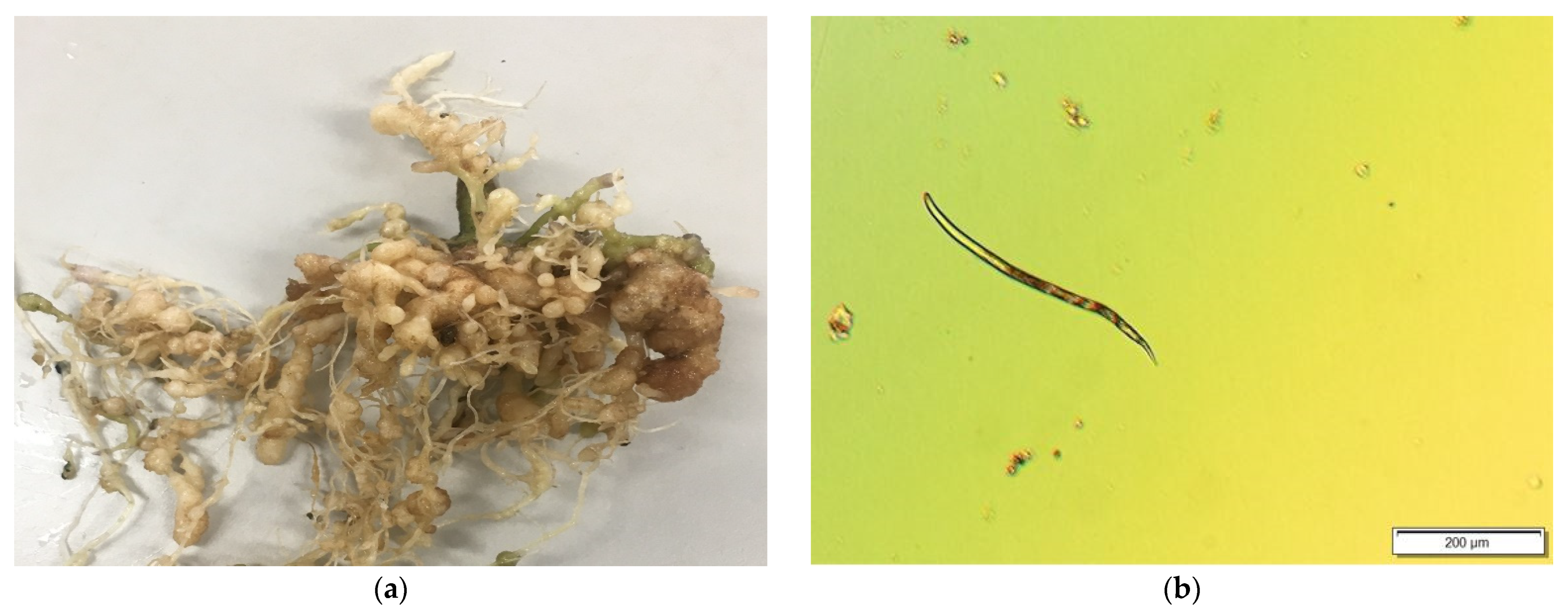
2.1. Soil Sample Preparation and Collection of Roots

Initially, tomato seeds were germinated indoors on a tray containing sand. The soil sample was prepared using a potting mix and sand (ratio of 1:1). The sand was used to avoid ingress of unwanted organisms and to create conditions suitable for sterilization. After four weeks, 70 tomato seedlings were transferred into white 600 mL plastic containers and placed in the greenhouse. The greenhouse was located at 24°54′5″ S, 152°18′45″ E (Central Queensland University Science Laboratory, Bundaberg Campus, Queensland, Australia, and the temperature was 14 ± 3 °C with 12 h light/12 h dark. The plants were inoculated with eggs of RKN (Meloidogyne incognita) five weeks after they were transplanted into the plastic containers. A few plant roots were inspected five weeks after the inoculation for the presence of root galls. The plant roots that had developed galls were deemed ready for nematode extraction

Extraction of nematodes from roots: After collecting the samples, plant stems were cut off and roots were separated. The roots were washed using tap water to remove sand and soil particles. Later, these roots were cut into smaller pieces (1 cm or less) and put into a 0.5% bleach solution (NaOCL) in a container for 5 min. Then, a modified version of Hussey [36] was used to extract RKN from root pieces. The roots were placed on a 135 µm-aperture sieve and stacked on a 25 µm-aperture sieve. The roots were washed with water and the residue was collected in a 25 µm aperture. The sieve with the residue was placed in water for 24 h. On the next day, the J2 sample in the water was used for image acquisition. The eggs of RKN were collected using 150 µm aperture. The residue was collected in the 25 µm aperture sieve and decanted on another 25 micron mini sieve and placed in a container. The sample floated for 24 h so that RKN could migrate down into the water from the sieve whereas soil particles remained on the sieve [37]. Then, the sample filtered from the mini sieve was used to observe RKN on the next day. This sample was termed as J2 from infected roots (JIR) because some of juveniles were found in the egg collection. Some eggs took a longer time to hatch. Juveniles hatched from eggs were retrieved on daily basis. Juveniles hatched from eggs after the egg collection process were termed as J2 from egg mass (JEM). Two samples were prepared for the size assessment: a sample of fresh JIR and another sample of the fresh JEM.

2.2. Image Acquisition

The images of the samples were captured to automate the RKN assessment. Five ml of the sample was placed in a 55 mm diameter petri dish, which was then mounted on the microscope stage. Many automated detection mechanisms have been implemented using a digital camera mounted on a microscope [17,18]. This study employed BX53 microscope with 4× objective lens and mounted digital camera. Images were captured on high contrast, ISO 200 sensitivity settings, with manual focus, and saved at 1600 × 1200 size. The head and tail of RKN were found to be transparent and colourless; hence, an appropriate acquisition setting was required to attain flawless segmentation. This study used a differential interference contrast (DIC) optical illumination technique because high contrast and high spatial resolution can capture the clear edges of RKN [38]. A total of 110 images of JIR and JEM were captured. Further, 570 images of JIR were acquired for investigation.

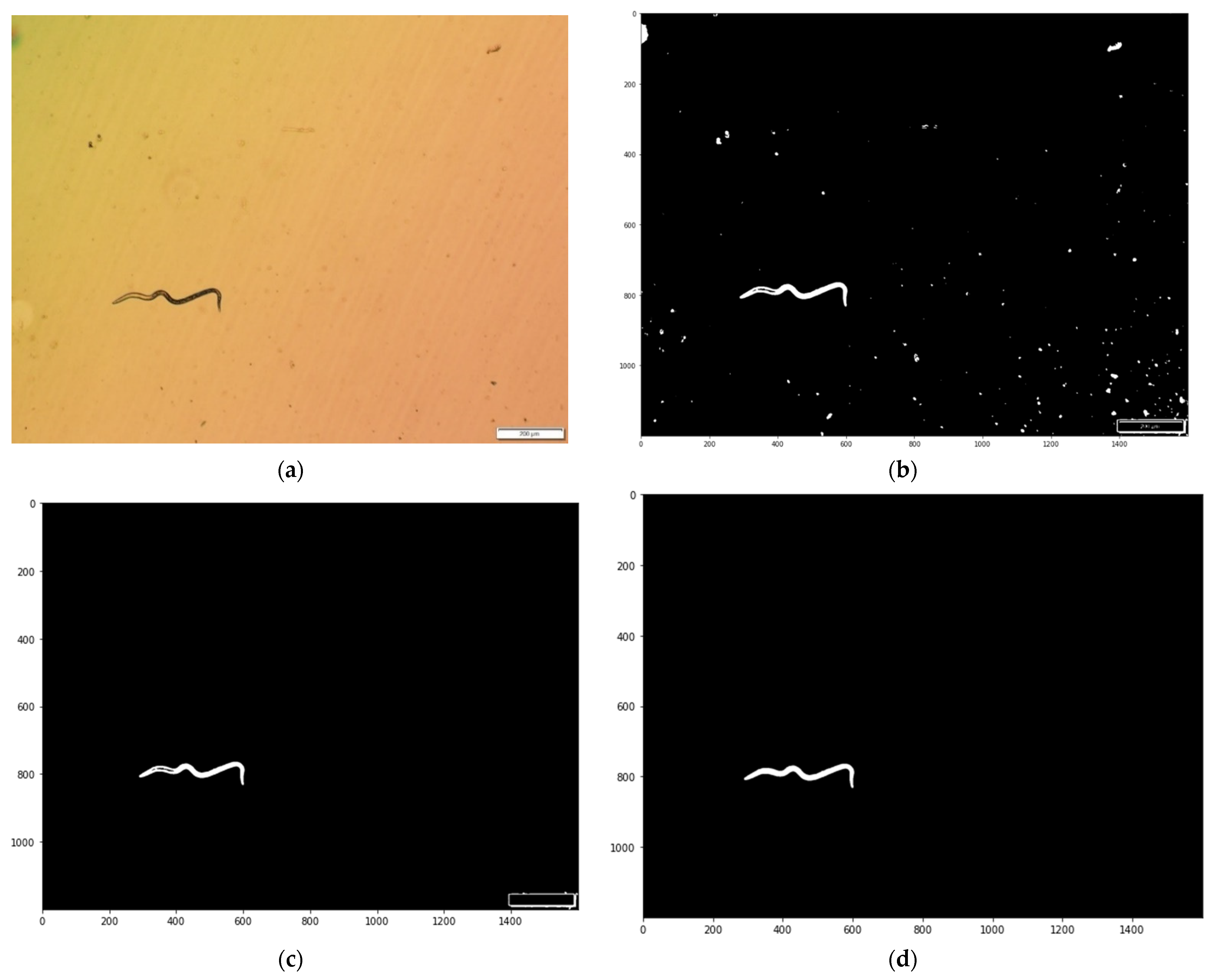
2.3. Image Processing

The images were processed and analysed to detect RKN in the image. First, images were pre-processed to separate noise, and then we applied segmentation. Subsequently, images were purified by removing dust particles before undertaking morphological operation. Ultimately, morphometric measurement of RKN was carried out to calculate size. All these steps were implemented using a new algorithm (Appendix A 

Table A2. Algorithm.

Algorithm

1. Load image (Img (x, y)) 2. Apply Gaussian filter to remove noise, Gaussian (Img (x, y), σ = 1) 3. Convert RGB image to gray, f (x, y) = Gray (Img (x, y)) 4. Apply triangle thresholding (T) to gray image $$Img\left(x,y\right)=\{\begin{array}{c}1,\hspace{0.17em}\hspace{0.17em}if f\left(x,y\right)>T\\ 0,\hspace{0.17em}\hspace{0.17em}if f\left(x,y\right)<T\end{array}$$ 5. Apply morphological small particle removal operation, remove_small_objects (Img (x, y), size = 2000) 6. Apply morphological closing operation to close boundary, morphology. Closing (Img (x, y), size = 5) 7. Fill holes in the image, binary_fill_holes Img (x, y)) 8. Find all contours(c) in the image Img (x, y)) 9. For each contour(c):     if (Minimum Area < contourArea(c) < Maximum Area)      a. Create mask of each contour      b. Compute Width, Length, Ratio and Area      c. if (Minimum Ratio < ratio < Maximum Ratio):        • contourArea(c) = RKN        • Save mask image and measurement      d. else        • contourArea(c) = Dust Particle or Rubbish 10. Save Image

).

2.3.1. Image Pre-Processing

This study used python programming language to process captured images. The images were preprocessed using a Gaussian filter to remove noise. A Gaussian filter is a linear filter that passes lower frequencies and removes normal distribution noise [39].

The one-dimensional Gaussian filter can be expressed as [40]:

$$Gx=\frac{1}{\sqrt{2\pi \sigma }}\mathit{exp}(-x^2/2{\sigma }^2)$$

(1)

where σ is variance of Gaussian filter.

As the input images were in RGB format (Figure 2a), it was necessary to convert them to gray to reduce colour complexity from three layers to single a layer. This reduced computational burden and avoided irrelevant information [41]. The image segmentation techniques were used to discriminate RKN from background soil particles in the image. Thresholding segmentation separates objects from the background [30]. This study implemented triangular thresholding based on the histogram, computed as the line between histogram peak and extreme point of the histogram. The threshold is the point at the longest distance between histogram and the line [42]. The image of RKN segmented using of triangle thresholding (Figure 2b). The segmentation technique can be defined as shown in Equation (2) [43].

$$T=T\left[x,y,P\left(x,y\right),f\left(x,y\right)\right]$$

(2)

where T is threshold value, (x, y) coordinate point of the threshold value p (x, y) and f (x, y) is the point of gray-level image pixel. The threshold of image g (x, y) can be defined as shown in Equation (3).

$$g\left(x,y\right)=\{\begin{array}{c}1, if f\left(x,y\right)>T\\ 0, if f\left(x,y\right)<T\end{array}$$

(3)

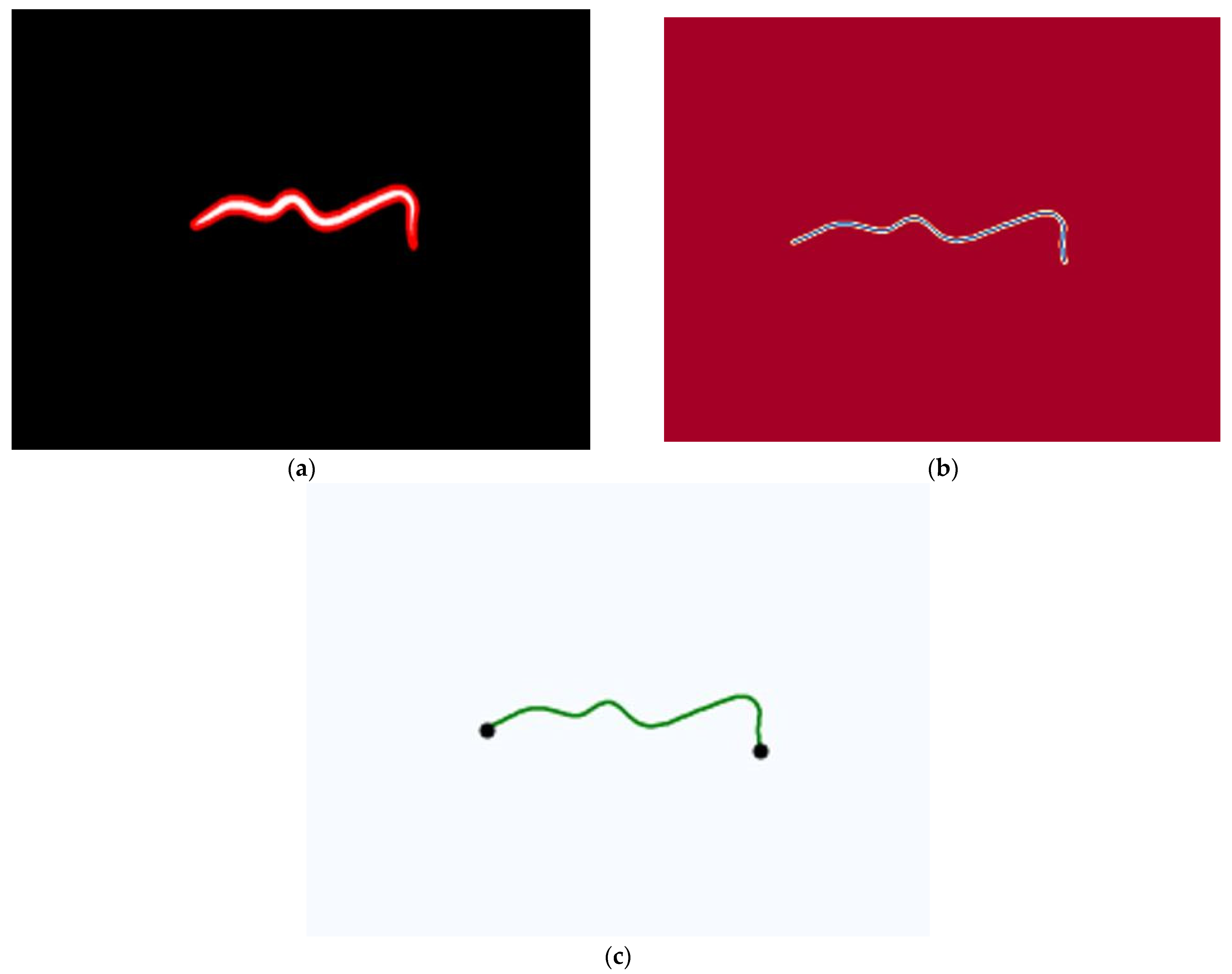
2.3.2. Image Purification

After segmentation of the images, the small soil particles were removed based on their size to reduce unnecessary computation. The particles having area less than the RKN minimum area were eliminated (Figure 3a). The morphological closing operation was performed on the image to restore missing edges. This closing operation was based on a morphological non-linear filter [44]. The closing operation smoothed contours of the image and filled in the thin gulf and small holes. It eliminated missing edges and then filled the holes [45] to obtain complete structures (Figure 3b). Subsequently, the contour of each object in the image was determined. The length, width, and the ratio of length to width were calculated as described in Section 2.3.3. The RKN was detected based on the ratio of length to width, and area. Its value range was specified from the automated measurement.

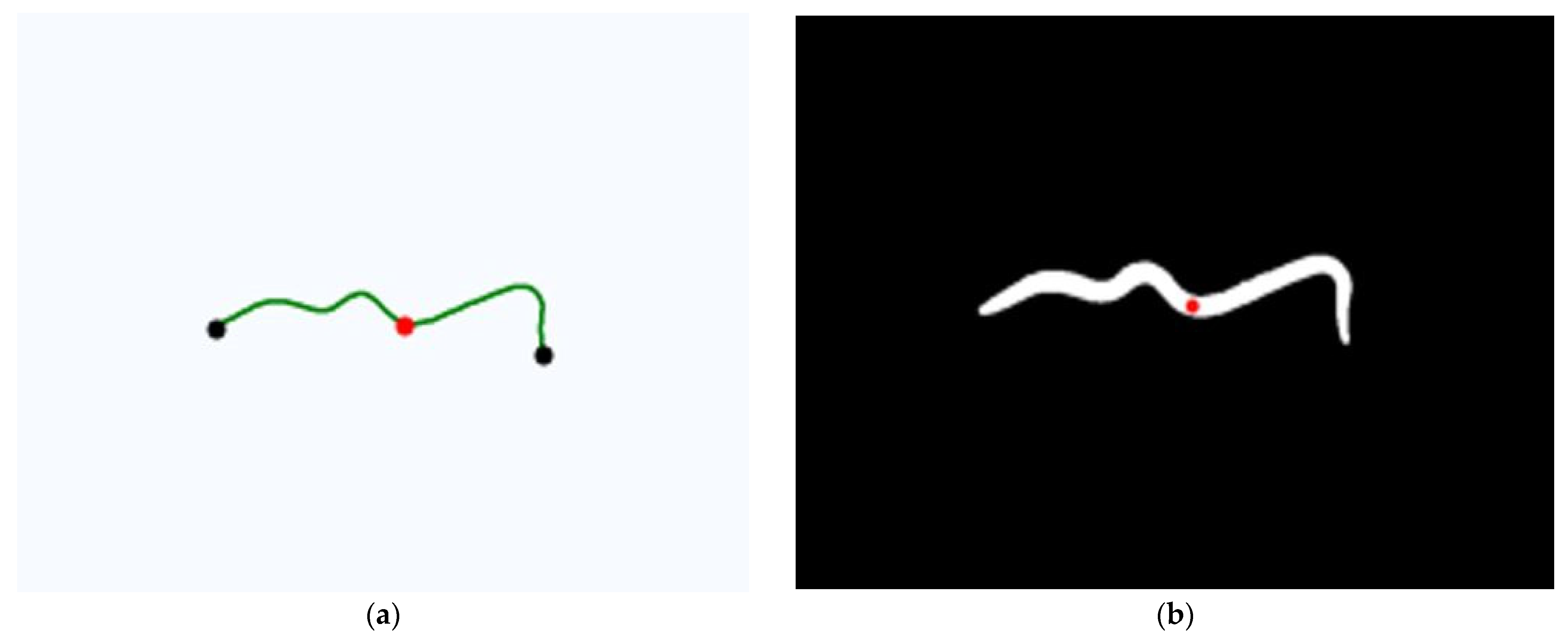
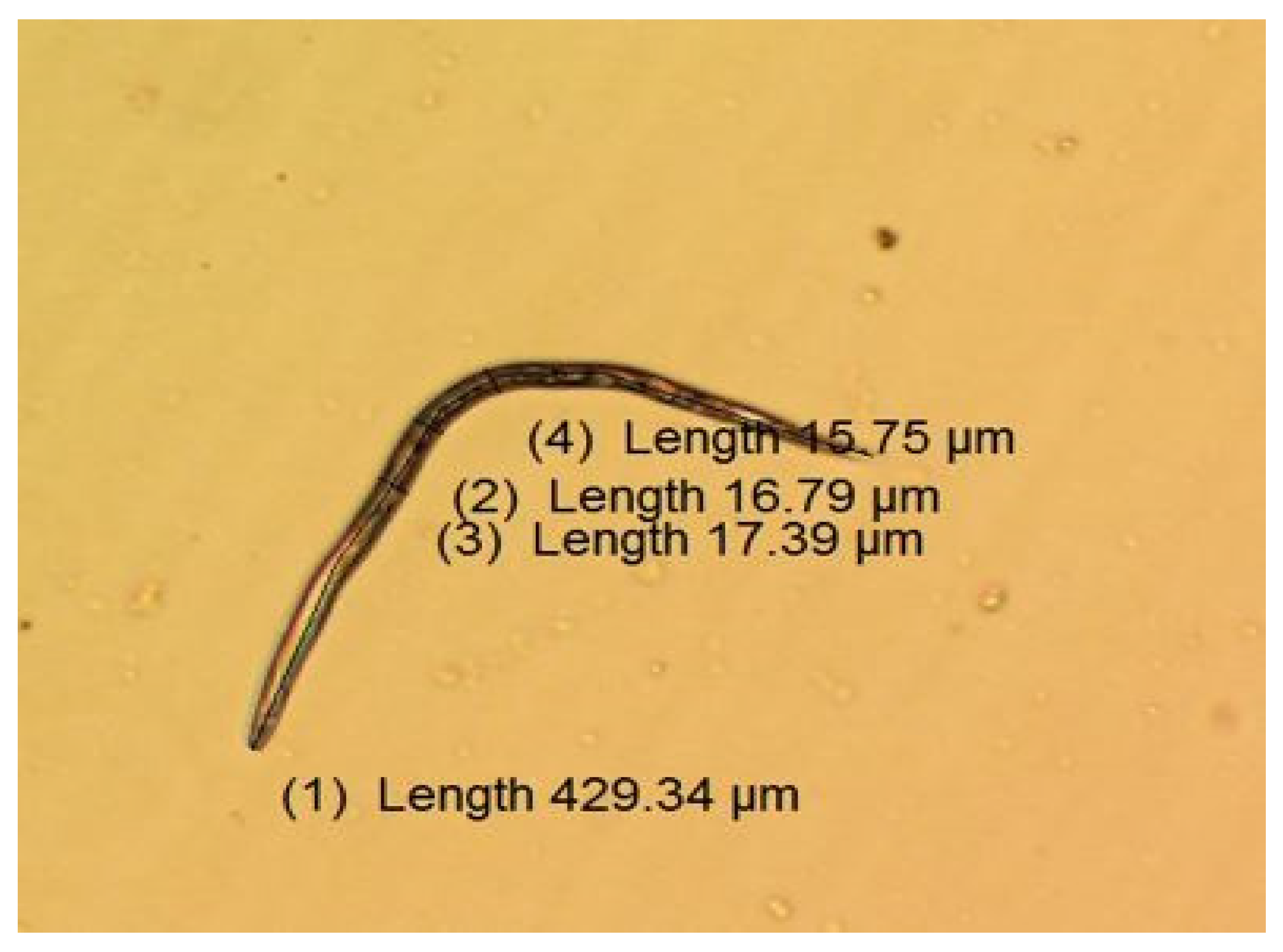
2.3.3. Morphometric Measurement

The length of RKN in the images was computed using three approaches: CA, TS, and SG. In the first approach, the contour of each RKN was detected (Figure 3a). Then, the perimeters of these contours were divided into two halves to obtain the length of RKN. In the second approach, the contour of RKN was converted to a thin structure to remove pixels from the edges until no more pixels could be eliminated without losing structure [46], and half of the thin structure perimeter was computed as length (Figure 3b). In the third method, the RKN in the image was transformed into a skeleton graph using the NetworkX Python package. Skeletons or thin structures are single-pixel representations of the object in the image (Appendix A). The end points of skeleton graphs were detected and the path length of each pair of end points was calculated based on the weight of the graph (Figure 3c). The path with the longest length was used to find the length of RKN. This method excludes unnecessary branches of the skeleton while computing the length of RKN.

The width of RKN was obtained using the medial axis average width. The medial axis of an object is defined as the collection of the point at the centre that has more than one closest point in the boundary or set of centres of the maximum inscribed disk [47]. Medial axis transform is a set of centre and radius pair of disks and is widely used in engineering and computer science. Medial axis transform can be applied to estimate the width of objects since it computes the distance to the boundary from all points of the medial axis. In this study, the width of RKN was estimated using medial axis distance at the middle of the RKN body length. To find the middle point of each RKN body, all the end points of skeleton graphs were detected. Then, the path length of each pair of end points was calculated using NetworkX Python package. Finally, the middle point of the longest path was computed, and the corresponding medial axis distance was used as width at the middle section of the RKN (Figure 4a,b).

3. Evaluation Criteria

The proposed method was evaluated using coefficient of determination (R²), root mean square error (RMSE), and analysis of variance (one way-ANOVA). The RMSE was used to measure prediction error between manual and automated measurement and counting. The R² was used to estimate how good the automated measurement or counting fitted in the regression model. One way-ANOVA was used to measure the statistical significance of group means.

3.1. Measurement Evaluation

The size of RKN was manually measured using Cell Sens software [48]. The length of RKN was measured from the head to tail part (Length (1) in Figure 5). The width of RKN was measured at equal intervals at the middle part of RKN (Length (2), Length (3), Length (4) in Figure 5) because the largest width is found in the middle of the body length (Figure 5) [17]. The average of these widths was computed as the actual width. The ratio was calculated as Length/Width and area of RKN as taken as Length × Width. These measurements were manually entered into a Microsoft Excel worksheet and saved in the CSV file format. The data of manual measurement included length, width, ratio (length/width), and area (length × width). The distribution of these data from JIR and JEM samples was analysed using density plots to find the minimum and maximum ratio and area (Figure 6 and Figure 7). The range of ratio and area used in the algorithm was fixed slightly larger than the maximum and minimum values of the ratio and area measurement. These parameters were used to find the automated measurement and to compare the results.

For automated measurement, the routine computed area of contours using OpenCV which is based on the Green Theorem [49]. The ratio was calculated as the body length to middle width. The automated computation of JIR and JEM found that the area value ranged between 3000–7000 pixels and ratio value ranged between 19–30. The minimum and maximum area of RKN was set to 3000–7000 pixels. Initially, the minimum and maximum ratio was set to 19–30. The range of ratios was increased to enable further investigation. The algorithm was further tested with a ratio range between 15–35, 12–35, 10–35, 8–35, 6–35, and 4–35.

3.2. Coefficient of Determination (R²)

The coefficient of determination is a common statistical approach to measure how effectively predicted value captures variability among true values [50]. The coefficient of determination is used to assess the goodness of regression model fit on observed data [51]. R² provides more facts compared to other evaluation metrics [52]. R² and RMSE are used for evaluating photon counting [53].

R² = 1 − SS_Regression/SS_total

where SS_Regression the sum of square due to regression that is the sum of square of difference between measurement and prediction. SS_total is total sum of square that is the sum of squares of the difference between measurement and their mean.

3.3. Root Mean Square Error (RMSE)

RMSE is defined as the squared root of mean square error. It is appropriate for measuring performance when errors are expected to be normally distributed [54]. RMSE measures accuracy by comparing prediction error of the models [55]. RMSE is used for counting crowds. It measures variation of residuals and is easily interpretable as a unit is the same as the dependent variable. RMSE is defined as

$$\mathrm{RMSE}=\sqrt{1/N{{\displaystyle \sum }}_{i=1}^N({\overline{\mathrm{y}}}_{\mathrm{i}}-{\mathrm{y}}_{\mathrm{i}})}$$

where N is total number of samples, ${\overline{\mathrm{y}}}_{\mathrm{i}}$ is predicted value, and y_i is actual value

3.4. One-Way Analysis of Variance (ANOVA)

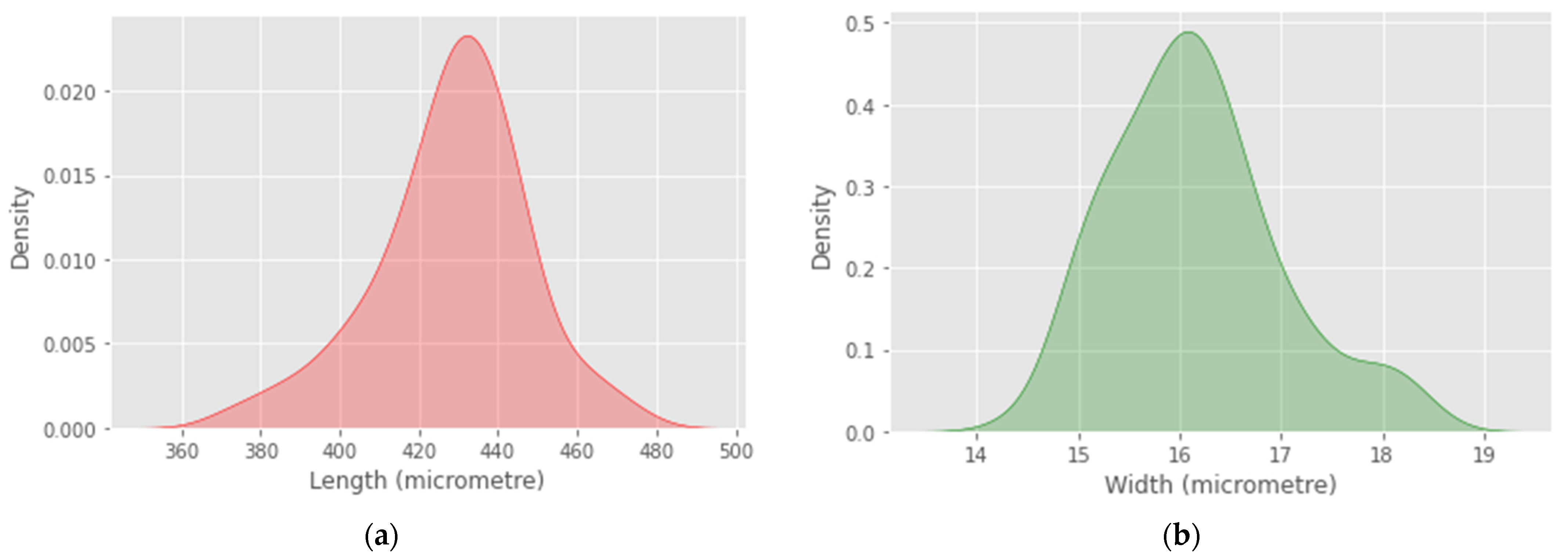
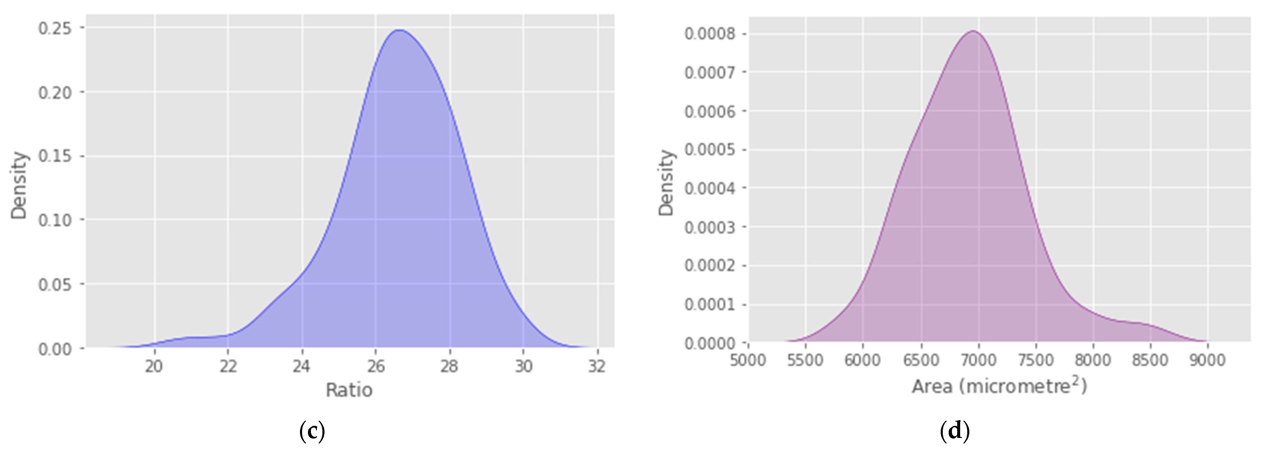
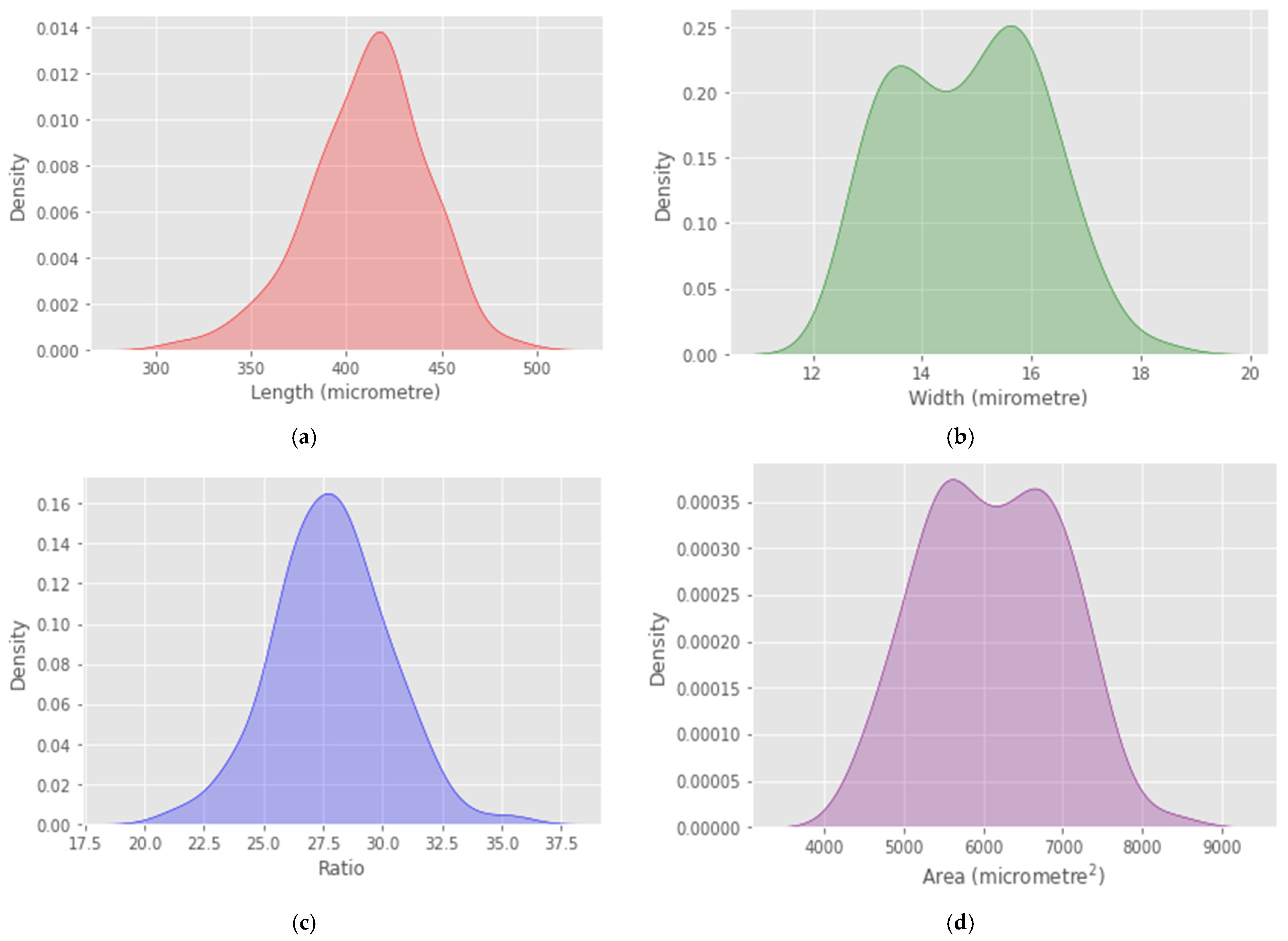
Analysis of variance is the assessment of means difference between two or more groups for statistical analysis. The null hypothesis states all group means are equal [56]. Rejecting the null hypothesis concludes that all group means are not equal [57]. To test the null hypothesis, we compare p-value with a significance level (α = 0.05); if p-value is less than or equal to the significance level then the difference between means is statistically significance. If the p-value is greater than the significance level, there is no statistical significance among group means. The null hypothesis (H1) and the alternative hypothesis (H2) is defined as follows [56]:

Hypothesis 1 (H1).

All means are equal, μ1 = μ2 = μ3.

Hypothesis 2 (H2).

Not all means are equal, μ1 ≠ μ2 or μ1 ≠ μ3 or μ2 ≠ μ3.

4. Results

The result of image analysis was evaluated using R², RMSE, and one way-ANOVA. The result was profound in RKN detection in both samples, the manual and automated length compared based on CA, TS, and SG of JIR (Figure 8). The CA and SG method attained the highest R² = 0.898 (

Table 2. Length comparison of J2 from infected roots (JIR) and J2 from egg masses (JEM).

Method	Sample	R2	RMSE
CA	JIR	0.898	14.237
	JEM	0.881	13.603
TS	JIR	0.875	23.975
	JEM	0.823	22.426
SG	JIR	0.898	24.501
	JEM	0.924	23.832

), whereas the TS method achieved R² = 0.875. Similar results were found from JEM (Figure 9). The SG-based computation achieved R² = 0.924. The CA- based computation attained R² = 0.881 while TS-based computation attained R² = 0.823. The RMSE of CA, TS, and SG was found to be 13.803, 22.426, and 23.832 in the JEM sample and 14.237, 23.975, and 24.501, respectively, in the JIR sample. The width and ratio calculated by the automated method were found to have an insignificant correlation to the manual width and the ratio of length to width. The ratio from manual and automated measurement was also compared using R² and RMSE (

Table 3. Ratio comparison of J2 from infected roots (JIR).

Ratio	R2	RMSE
CA	0.220	2.137
TS	0.227	2.528
SG	0.206	2.590

). The manual width and automated width comparison measurements in both samples were found to be insignificant. The width computation revealed R² = 0.09 with RMSE = 1.15 from JIR and R² = 0.06 with RMSE = 2.482 JEM.

Further, the three methods were used to detect RKN from JEM sample in 517 images consisting of 1953 RKN. The R² assessed to compare manual and automated counting of CA, TS, SG methods were 0.857, 0.835, and 0.828, respectively (

Table 4. Count comparison with ratio variation.

Ratio	Method	R2	RMSE	Misidentified	Undetected
19–30	CA	0.857	0.481	3	97
	TS	0.835	0.520	2	110
	SG	0.828	0.533	3	114
15–35	CA	0.961	0.232	6	20
	TS	0.959	0.236	8	17
	SG	0.961	0.232	6	20
12–35	CA	0.966	0.215	11	9
	TS	0.961	0.232	6	20
	SG	0.967	0.210	8	13
10–35	CA	0.965	0.219	13	8
	TS	0.958	0.240	16	8
	SG	0.973	0.191	7	10
8–35	CA	0.947	0.271	22	8
	TS	0.945	0.278	23	7
	SG	0.969	0.206	11	9
6–35	CA	0.927	0.326	33	6
	TS	0.919	0.346	39	7
	SG	0.961	0.232	17	9
4–35	CA	0.872	0.452	68	6
	TS	0.881	0.435	67	5
	SG	0.949	0.267	27	8

). The RMSE of CA, TS, and SG methods were 0.481, 0.520, and 0.533, respectively. The CA, TS and SG computation methods showed three, two and three misidentifications, respectively. On the other hand, CA method missed 97 RKN. Similarly, TS could not detect 110 RKN, and SG method missed 114 RKN. The one way- ANOVA test performed on count from CA, TS, and SG method found F-statistic = 4.440 and p-value = 0.004. In addition, three methods were investigated with ratio variation from 19–30,15–35, 12–35, 10–35, 8–35, 6–35, and 4–35 (Table 4). The ratio between 10–35 was found to have the lowest number of misidentified and missed RKN. The SG method misidentified seven RKN and ten RKN were not detected, whereas the TS method did not identify sixteen RKN and eight RKN were missed. Similarly, the CA method did not detect eight RKN and misidentified thirteen RKN.

5. Discussion

The manual measurement and counting of nematodes is a common and relatively simple, labour-intensive, and time-consuming process. The manual approach took around 2–3 min to measure the RKN precisely because the head and tail parts of RKN are transparent. On the other hand, the automated method used to count RKN in the images showed the proposed model is a good fit for data with high R². The optimal range of ratio was observed at 10–35 for the detection and counting of RKN. Automated counting and measurement approaches are time-efficient and accurate. This study assessed RKN size of JIR and JEM extracted from tomato plant roots and built a novel algorithm to detect RKN with three distinct approaches to calculate length.

In this study, image analysis techniques were applied to automate the RKN measurement and quantification process. Root-knot nematodes in each image were analysed using computer vision methods. There is no other approach in the literature that has used this method to detect RKN or even other nematodes. The length of RKN is computed as the perimeter of CA, TS, and SG. The SG method was estimated using the NetworkX Python package. The SG method showed the highest correlation in both samples, whereas the TS method achieved the lowest correlation, slightly. The images of JEM had more soil particles than those obtained from JIR because egg collection also includes soil particles. The results observed from JEM also had similar outcomes as JIR. The comparison of RMSE also revealed negligible differences between JIR and JEM. The correlation of skeleton graph-based computation increased to R² = 0.924. The CA method correlation was slightly reduced to R² = 0.881. Similarly, the TS method decreased to R² = 0.823. The decline of correlation in the CA and TS methods is because of the deformation of RKN shape. This shape deformation normally originated from the attachment of small soil particles or microorganisms (fungus) to the RKN body. This changed the original contour, and thus the skeleton structure of the RKN. Hence, inappropriate branches were created in the skeleton structure, which then attached additional endpoints in the graph. The thinning operation reduced the sizes of soil particles and matched RKN size, resulting in a slight reduction in correlation with JEM. The SG method showed the highest correlation in terms of R² in both samples. This method is more robust even in dirty images. The method excludes irrelevant branches of the skeleton while computing the length of the skeleton graph. This finding confirmed that the SG method effectively represents the complex structure of the object and preserves the topologic and geometric properties of RKN more accurately [58]. There was a high correlation between the length of RKN measured by the manual method and that obtained using the machine method. The Naïve Bayes classifier and Linear Discriminant Analysis attained 96.1% and 93.5% accuracy, whereas the SG method achieved 97.3% [23]. Similarly, the detection rate was 87% in [19], whereas the proposed method outperformed it. The fluorescence-based imaging system revealed R² = 0.95, whereas the proposed CA, TS, and SF methods achieved better results than this method [21]. In addition, around 92% of RKN measurement of satisfied length specification written in the taxonomic literature of root-knot incognita. A similar result was found with automated measurement of root-knot incognita. Few root-knot nematodes have slightly higher length than the specification. This might be influenced by duration of time chosen to extract nematodes and the environment provided by the host plant.

On the other hand, a negligible correlation between the manual and automated measurements in the computation of the width and ratio was noted. The correlation was slightly higher than width because the length is proportional to the ratio. It still had negligible correlation. A similar trivial correlation of the width was observed in the assessment of biomass of nematodes [17]. This situation also occurred while studying the automated method to analyse MRI images [59]. In addition to these, width inconsistency may be because cross-sectional values are more susceptible to errors than longitudinal values.

The algorithm was further tested on 517 images which showed an excellent correlation with manual counting. The CA method had the highest correlation between manual and automated counting with R² = 0.857 and RMSE = 0.481; however, three false RKN detected and 97 RKN unrecognized. The TS method discerned two dust particles and 110 RKN missed. Similarly, the SG method missed 114 RKN and three were misidentified. The one-way ANOVA test found F-statistic = 4.440 and p-value = 0.004, which is less than significance level. Thus, the difference between the means of these counting methods is statistically significant. These RKN were disregarded because of self-tangled or overlapped structure due to which length of RKN varies. Thus, the value of the ratio was changed to include these self-tangled RKN.

The algorithm achieved the highest R² and a smaller number of false detections and missed RKN with a ratio range between 10 to 35. These results found that the SG method had the highest correlation and lowest prediction errors as compared to other methods. The SG method showed good performance in highly cluttered images. The skeleton algorithm has been extensively used in shape recognition and analysis, path and motion tracking, character recognition, and medical imaging applications such as stenosis detection, tracking and analysis of the anatomic structure, and object morphology characterization [60]. The Skan Python Library builds skeleton-sized or thinned object graphs and provides branch information from skeleton images [61]. The lengths RKN are computed as the largest length in the skeleton graph network. However, this study implemented a skeleton graph structure to measure length. The thin structure of contour is used to convert graph structure to avoid unnecessary branches. This supported the achievement of the accurate length of the skeleton graph structure. The limitation of the proposed study is that it is based on the measurement of RKN size.

Prior measurement of RKN (manual or automated) is necessary to find the value of morphological parameters. The suspension required to keep in the mini sieve for 24 h, to separate RKN and dust particles. Further, the proposed method could not detect multiple overlapped RKN.

This method is particularly based on the study of M. incognita. Other common RKN species found in Queensland, Australia and infesting tomatoes are M. incognita, M. javanica, M. arenaria, and M. hapla [1]. The algorithm developed in this study detects nematodes in terms of length to width ratio. As the J2 length of these common species is almost similar, the algorithm detects these common species with similar length to width ratios. The approach and specifications used in this study are based on the J2 stage of the RKN. This is the most infectious stage of the RKN [62,63].

6. Conclusions

The proposed method estimates RKN size and enumerates it based on length and width. The length of RKN is computed using three methods. The contour arc (CA), thin structure (TS), and skeleton graph (SG) methods were implemented to automate the measurement of RKN. The skeleton graph structure was the most accurate in detecting RKN. This method can be used for the assessment of the nematode population for rapid management. This study may be used to model and detect the irregular and complex structure of objects. The algorithm can be implemented to count microorganisms with irregular shapes. In addition, the optimal range of ratio was found at 10–35 for detecting RKN in an image. The presented technique can be very useful in discerning and quantifying other nematodes and automating image labeling tasks for machine learning with quality images. Although the method proposed in this study was able to detect and count RKN, it could not detect nematodes attached to large soil particles. Thus, roots must be cleaned properly during sample processing. Future work may investigate effective ways to remove soil particles. Further, different segmentation techniques can be applied to improve object detection.

A perspective study could be on overlapped structure of RKN and use spectral technology to detect RKN and similar microorganisms.

References

1. Department of Agriculture and Fisheries. Root-Knot Nematode. Available online: https://www.daf.qld.gov.au/business-priorities/agriculture/plants/fruit-vegetable/insect-pests/root-knot-nematode (accessed on 20 October 2021).
2. Nicol, J.; Turner, S.; Coyne, D.; den Nijs, L.; Hockland, S.; Maafi, Z.T. Current nematode threats to world agriculture. In Genomics and Molecular Genetics of Plant-Nssematode Interactions; Jones, J., Gheysen, G., Fenoll, C., Eds.; Springer: Berlin/Heidelberg, Germany, 2011; pp. 21–43. [Google Scholar]
3. Elling, A.A. Major emerging problems with minor Meloidogyne species. Phytopathology 2013, 103, 1092–1102. [Google Scholar] [CrossRef] [PubMed] [Green Version]
4. Jones, J.T.; Haegeman, A.; Danchin, E.G.; Gaur, H.S.; Helder, J.; Jones, M.G.; Kikuchi, T.; Manzanilla-López, R.; Palomares-Rius, J.E.; Wesemael, W.M. Top 10 plant-parasitic nematodes in molecular plant pathology. Mol. Plant Pathol. 2013, 14, 946–961. [Google Scholar] [CrossRef] [PubMed]
5. Seid, A.; Fininsa, C.; Mekete, T.; Decraemer, W.; Wesemael, W.M.L. Tomato (Solanum lycopersicum) and root-knot nematodes (Meloidogyne spp.)—A century-old battle. Nematology 2015, 17, 995–1009. [Google Scholar] [CrossRef] [Green Version]
6. Jagdale, G.; Arnold-Smith, L.C. Sampling for Plant-Parasitc Nematodes Identification and Diagnosis. Available online: https://athenaeum.libs.uga.edu/bitstream/handle/10724/34728/NemaSamplingGuideApr2011.pdf?sequence=1 (accessed on 7 April 2021).
7. Vezina, A. Root-Knot Nematodes. Available online: https://www.promusa.org/Root-knot+nematodes (accessed on 28 August 2021).
8. Hunt, D.J.; Handoo, Z.A. Root-Knot Nematodes; Perry, R.N., Moens, M., Starr, J.L., Eds.; CABI: Wallingford, UK, 2009. [Google Scholar]
9. Moens, M.; Perry, R.N.; Starr, J.L. Meloidogyne species—A diverse group of novel and important plant parasites. In Root-Knot Nematodes; Perry, R.N., Moens, M., Starr, J.L., Eds.; CABI: Wallingford, UK, 2009; Volume 1, p. 483. [Google Scholar]
10. Mitkowski, N.A.; Adawi, G.S. Root-knot Nematode. Plant Health Instr. 2003. [Google Scholar] [CrossRef]
11. Eisenback, J.D.; Hunt, D.J. General Morphology In Root-Knot Nematodes; Starr, J.L., Moens, M., Perry, R.N., Eds.; CABI: Wallingford, UK, 2009. [Google Scholar]
12. De Man, J. Die Einheimischen, Frei in der Reinen Erde und im Süssen Wasser Lebende Nematoden; Brill: Leiden, The Netherlands, 1880; Volume 5, pp. 1–104. [Google Scholar]
13. De Man, J.G. Onderzoekingen over Vrij in de Aarde Levende Nematoden; Gravenhage: The Hague, The Netherlands, 1877. [Google Scholar]
14. Chiu, M.T.; Xu, X.; Wei, Y.; Huang, Z.; Schwing, A.; Brunner, R.; Khachatrian, H.; Karapetyan, H.; Dozier, I.; Rose, G.; et al. Agriculture-Vision: A Large Aerial Image Database for Agricultural Pattern Analysis. In Proceedings of the IEEE/CVF Conference on Computer Vision and Pattern Recognition, Seattle, WA, USA, 14–19 June 2020; pp. 2828–2838. [Google Scholar]
15. Gomes, J.F.S.; Leta, F.R. Applications of computer vision techniques in the agriculture and food industry: A review. Eur. Food Res. Technol. 2012, 235, 989–1000. [Google Scholar] [CrossRef]
16. Tian, H.; Wang, T.; Liu, Y.; Qiao, X.; Li, Y. Computer vision technology in agricultural automation—A review. Inf. Process. Agric. 2020, 7, 1–19. [Google Scholar] [CrossRef]
17. Mazurkiewicz, M.; Górska, B.; Jankowska, E.; Włodarska-Kowalczuk, M. Assessment of nematode biomass in marine sediments: A semi-automated image analysis method. Limnol. Oceanogr. Methods 2016, 14, 816–827. [Google Scholar] [CrossRef]
18. Moore, B.T.; Jordan, J.M.; Baugh, L.R. WormSizer: High-throughput analysis of nematode size and shape. PLoS ONE 2013, 8, e57142. [Google Scholar] [CrossRef] [Green Version]
19. Kurtulmuş, F.; Ulu, T.C. Detection of dead entomopathogenic nematodes in microscope images using computer vision. Biosyst. Eng. 2014, 118, 29–38. [Google Scholar] [CrossRef]
20. Puckering, T.; Thompson, J.; Sathyamurthy, S.; Sukumar, S.; Shapira, T.; Ebert, P. Automated Wormscan. F1000Res 2017, 6, 192. [Google Scholar] [CrossRef]
21. Wählby, C.; Kamentsky, L.; Liu, Z.H.; Riklin-Raviv, T.; Conery, A.L.; O’Rourke, E.J.; Sokolnicki, K.L.; Visvikis, O.; Ljosa, V.; Irazoqui, J.E.; et al. An image analysis toolbox for high-throughput C. elegans assays. Nat. Methods 2012, 9, 714–716. [Google Scholar] [CrossRef] [PubMed] [Green Version]
22. Brown, S.; Yeckel, G.; Heinz, R.; Clark, K.; Sleper, D.; Mitchum, M.G. A High-Throughput Automated Technique for Counting Females of Heterodera glycines using a Fluorescence-Based Imaging System. J. Nematol. 2010, 42, 201–206. [Google Scholar]
23. Oscar, G.; Maria, F.A.; Moreno-Vazquez, S. Quantitative evaluation of Heterodera avenae females in soil and root extracts by digital image analysis. Crop. Prot. 2016, 81, 85–91. [Google Scholar] [CrossRef]
24. Vagelas, I.; Pembroke, B.; Gowen, S.R. Techniques for image analysis of movement of juveniles of root-knot nematodes encumbered with Pasteuria penetransspores. Biocontrol. Sci. Technol. 2011, 21, 239–250. [Google Scholar] [CrossRef]
25. Qazi, F.; Khalid, A.; Poddar, A.; Tetienne, J.-P.; Nadarajah, A.; Aburto-Medina, A.; Shahsavari, E.; Shukla, R.; Prawer, S.; Ball, A.S. Real-time detection and identification of nematode eggs genus and species through optical imaging. Sci. Rep. 2020, 10, 7219. [Google Scholar] [CrossRef]
26. Akintayo, A.; Tylka, G.L.; Singh, A.K.; Ganapathysubramanian, B.; Singh, A.; Sarkar, S. A deep learning framework to discern and count microscopic nematode eggs. Sci. Rep. 2018, 8, 9145. [Google Scholar] [CrossRef] [PubMed]
27. Rauf, H.T.; Saleem, B.A.; Lali, M.I.U.; Khan, M.A.; Sharif, M.; Bukhari, S.A.C. A citrus fruits and leaves dataset for detection and classification of citrus diseases through machine learning. Data Brief 2019, 26, 104340. [Google Scholar] [CrossRef] [PubMed]
28. Almadhor, A.; Rauf, H.T.; Lali, M.I.U.; Damaševičius, R.; Alouffi, B.; Alharbi, A. AI-Driven Framework for Recognition of Guava Plant Diseases through Machine Learning from DSLR Camera Sensor Based High Resolution Imagery. Sensors 2021, 21, 3830. [Google Scholar] [CrossRef] [PubMed]
29. Khan, W. Image Segmentation Techniques: A Survey. J. Image Graph. 2014, 166–170. [Google Scholar] [CrossRef] [Green Version]
30. Sahoo, P.K.; Soltani, S.; Wong, A.K.C. A survey of thresholding techniques. Comput. Vis. Graph. Image Process. 1988, 41, 233–260. [Google Scholar] [CrossRef]
31. Netto, A.F.A.A.; Martins, R.N.; de Souza, G.S.A.; Araújo, G.D.M.; de Almeida, S.L.H.; Capelini, V.A. Segmentation of Rgb Images Using Different Vegetation Indices and Thresholding Methods. Nativa 2018, 6, 389–394. [Google Scholar] [CrossRef]
32. Hakim, A.; Mor, Y.; Toker, I.A.; Levine, A.; Neuhof, M.; Markovitz, Y.; Rechavi, O. WorMachine: Machine learning-based phenotypic analysis tool for worms. BMC Biol. 2018, 16, 8. [Google Scholar] [CrossRef] [Green Version]
33. Holladay, B.H.; Willett, D.S.; Stelinski, L.L. High throughput nematode counting with automated image processing. BioControl 2015, 61, 177–183. [Google Scholar] [CrossRef]
34. Tajima, R.; Kato, Y. Comparison of threshold algorithms for automatic image processing of rice roots using freeware ImageJ. Field Crop Res. 2011, 121, 460–463. [Google Scholar] [CrossRef]
35. Patil, S.B.; Bodhe, S.K. Leaf disease severity measurement using image processing. Int. J. Eng. Technol. 2011, 3, 297–301. [Google Scholar]
36. Hussey, R. A comparison of methods of collecting inocula of Meloidogyne spp., including a new technique. Plant Dis. Rep. 1973, 57, 1025–1028. [Google Scholar]
37. Van Bezooijen, J. Methods and Techniques for Nematology; Wageningen University: Wageningen, The Netherlands, 2006. [Google Scholar]
38. Fu, D.; Oh, S.; Choi, W.; Yamauchi, T.; Dorn, A.; Yaqoob, Z.; Dasari, R.R.; Feld, M.S. Quantitative DIC microscopy using an off-axis self-interference approach. Opt. Lett. 2010, 35, 2370–2372. [Google Scholar] [CrossRef] [PubMed] [Green Version]
39. Wang, M.; Zheng, S.; Li, X.; Qin, X. A new image denoising method based on Gaussian filter. In Proceedings of the 2014 International Conference on Information Science, Electronics and Electrical Engineering, Sapporo, Japan, 26–28 April 2014; pp. 163–167. [Google Scholar]
40. Deng, G.; Cahill, L. An adaptive Gaussian filter for noise reduction and edge detection. In Proceedings of the 1993 IEEE Conference Record Nuclear Science Symposium and Medical Imaging Conference, San Francisco, CA, USA, 30 October–6 November 1993; pp. 1615–1619. [Google Scholar]
41. Kanan, C.; Cottrell, G.W. Color-to-grayscale: Does the method matter in image recognition? PLoS ONE 2012, 7, e29740. [Google Scholar]
42. Zack, G.W.; Rogers, W.E.; Latt, S.A. Automatic measurement of sister chromatid exchange frequency. J. Histochem. Cytochem. 1977, 25, 741–753. [Google Scholar] [CrossRef] [PubMed]
43. Al-Amri, S.S.; Kalyankar, N.V. Image segmentation by using threshold techniques. arXiv 2010, arXiv:1005.4020. [Google Scholar]
44. Maragos, P.; Schafer, R. Morphological filters—Part I: Their set-theoretic analysis and relations to linear shift-invariant filters. IEEE Trans. Acoust. Speech Signal Process. 1987, 35, 1153–1169. [Google Scholar] [CrossRef]
45. Maragos, P. Morphological filtering for image enhancement and feature detection. In The Image and Video Processing Handbook; Academic Press: Cambridge, MA, USA, 2005; pp. 135–156. [Google Scholar]
46. Zhang, T.Y.; Suen, C.Y. A fast parallel algorithm for thinning digital patterns. Commun. ACM 1984, 27, 236–239. [Google Scholar] [CrossRef]
47. Choi, H.I.; Choi, S.W.; Moon, H.P. Mathematical theory of medial axis transform. Pac. J. Math. 1997, 181, 57–88. [Google Scholar] [CrossRef]
48. Olympus. cellSens Life Science Imaging Software. Available online: https://investigacion.us.es/docs/web/files/manual_cellsens_en.pdf (accessed on 6 November 2020).
49. Harrison, J.; Norton, A. The Gauss-Green theorem for fractal boundaries. Duke Math. J. 1992, 67, 575–588. [Google Scholar] [CrossRef] [Green Version]
50. Sarkar, S.; Lund, S.P.; Vyzasatya, R.; Vanguri, P.; Elliott, J.T.; Plant, A.L.; Lin-Gibson, S. Evaluating the quality of a cell counting measurement process via a dilution series experimental design. Cytotherapy 2017, 19, 1509–1521. [Google Scholar] [CrossRef] [PubMed]
51. Reisinger, H. The impact of research designs on R2 in linear regression models: An exploratory meta-analysis. J. Empir. Gen. Mark. Sci. 1997, 2, 1–12. [Google Scholar]
52. Chicco, D.; Warrens, M.J.; Jurman, G. The coefficient of determination R-squared is more informative than SMAPE, MAE, MAPE, MSE and RMSE in regression analysis evaluation. PeerJ Comput. Sci. 2021, 7, e623. [Google Scholar] [CrossRef]
53. Si-Mohamed, S.; Bar-Ness, D.; Sigovan, M.; Tatard-Leitman, V.; Cormode, D.P.; Naha, P.C.; Coulon, P.; Rascle, L.; Roessl, E.; Rokni, M. Multicolour imaging with spectral photon-counting CT: A phantom study. Eur. Radiol. Exp. 2018, 2, 34. [Google Scholar] [CrossRef]
54. Chai, T.; Draxler, R.R. Root mean square error (RMSE) or mean absolute error (MAE)?—Arguments against avoiding RMSE in the literature. Geosci. Model Dev. 2014, 7, 1247–1250. [Google Scholar] [CrossRef] [Green Version]
55. Neill, S.P.; Hashemi, M.R. Ocean Modelling for Resource Characterization. In Fundamentals of Ocean Renewable Energy; Neill, S.P., Hashemi, M.R., Eds.; Academic Press: Cambridge, MA, USA, 2018; pp. 193–235. [Google Scholar]
56. Kim, T.K. Understanding one-way ANOVA using conceptual figures. Korean J. Anesthesiol. 2017, 70, 22. [Google Scholar] [CrossRef] [Green Version]
57. Faraway, J.J. Practical Regression and ANOVA Using R; University of Bath: Bath, UK, 2002; Volume 168. [Google Scholar]
58. Saha, P.K.; Borgefors, G.; di Baja, G.S. A survey on skeletonization algorithms and their applications. Pattern Recognit. Lett. 2016, 76, 3–12. [Google Scholar] [CrossRef]
59. Hsu, Y.-Y.; Schuff, N.; Du, A.-T.; Mark, K.; Zhu, X.; Hardin, D.; Weiner, M.W. Comparison of automated and manual MRI volumetry of hippocampus in normal aging and dementia. J. Magn. Reson. Imaging 2002, 16, 305–310. [Google Scholar] [CrossRef] [PubMed]
60. Saha, P.K.; Udupa, J.K. Optimum image thresholding via class uncertainty and region homogeneity. IEEE Trans. Pattern Anal. Mach. Intell. 2001, 23, 689–706. [Google Scholar] [CrossRef]
61. Nunez-Iglesias, J.; Blanch, A.J.; Looker, O.; Dixon, M.W.; Tilley, L. A new Python library to analyse skeleton images confirms malaria parasite remodelling of the red blood cell membrane skeleton. PeerJ 2018, 6, e4312. [Google Scholar] [CrossRef] [Green Version]
62. Curtis, R.H.; Robinson, A.F.; Perry, R.N. Hatch and host location. In Root-Knot Nematodes; Perry, R.N., Moens, M., Starr, J.L., Eds.; CABI: Wallingford, UK, 2009; Volume 1, pp. 139–162. [Google Scholar]
63. Caillaud, M.-C.; Dubreuil, G.; Quentin, M.; Perfus-Barbeoch, L.; Lecomte, P.; de Almeida Engler, J.; Abad, P.; Rosso, M.-N.; Favery, B. Root-knot nematodes manipulate plant cell functions during a compatible interaction. J. Plant Physiol. 2008, 165, 104–113. [Google Scholar] [CrossRef]
Figure 1. (a) Root galls of a tomato plant (b) Juvenile (J2) of root-knot nematode.
Agronomy 11 02372 g001
Figure 2. Image pre-processing and purification (a) Red, Green, and Blue (RGB) image of root-knot nematode (b) Segmentation of Red, Green, and Blue (RGB) image using triangular thresholding (c) Image after removing small particles (d) Image after morphological closing and filling of holes.
Agronomy 11 02372 g002
Figure 3. Morphometric view of RKN (juvenile) (a) Red contour along RKN juvenile edge (b) Thinned contour structure of RKN (juvenile) (c) Skeleton graph structure of RKN (juvenile).
Agronomy 11 02372 g003
Figure 4. (a) Skeleton graph structure of RKN with middle point (b) Binarised image of RKN with middle point.
Agronomy 11 02372 g004
Figure 5. RKN (J2) image with measurement.
Agronomy 11 02372 g005
Figure 6. Manual measurement distribution of J2 from infected roots (JIR) (a) Distribution of length (b) Distribution of width (c) Distribution of ratio (d) Distribution of area.
Agronomy 11 02372 g006aAgronomy 11 02372 g006b
Figure 7. Manual measurement distribution of J2 from egg mass (JEM) (a) Distribution of length (b) Distribution of width (c) Distribution of ratio (d) Distribution of area.
Agronomy 11 02372 g007
Figure 8. Manual and machine length comparison of J2 from infected roots (JIR) (a) contour arc (CA); (b) thin structure (TS); (c) skeleton graph (SG).
Agronomy 11 02372 g008
Figure 9. Manual and machine length comparison of J2 from egg masses (JEM) (a) contour arc (CA); (b) thin structure (TS); (c) skeleton graph (SG).
Agronomy 11 02372 g009