Evaluating Heathland Restoration Belowground Using Different Quality Indices of Soil Chemical and Biological Properties

 , , , , and
Abstract
:1. Introduction
2. Materials and Methods
2.1. Site Description
2.2. Soil Sampling
2.3. Vegetation Survey
2.4. Chemical Variables
2.5. Biological Variables
2.5.1. Soil Microbial Biomass
2.5.2. Community-Level Physiological Profiles
2.5.3. Phospholipid Fatty Acid Analysis
2.5.4. Soil Fauna
2.6. Heathland Restoration Index (HRI)
2.7. Statistical Analysis
3. Results
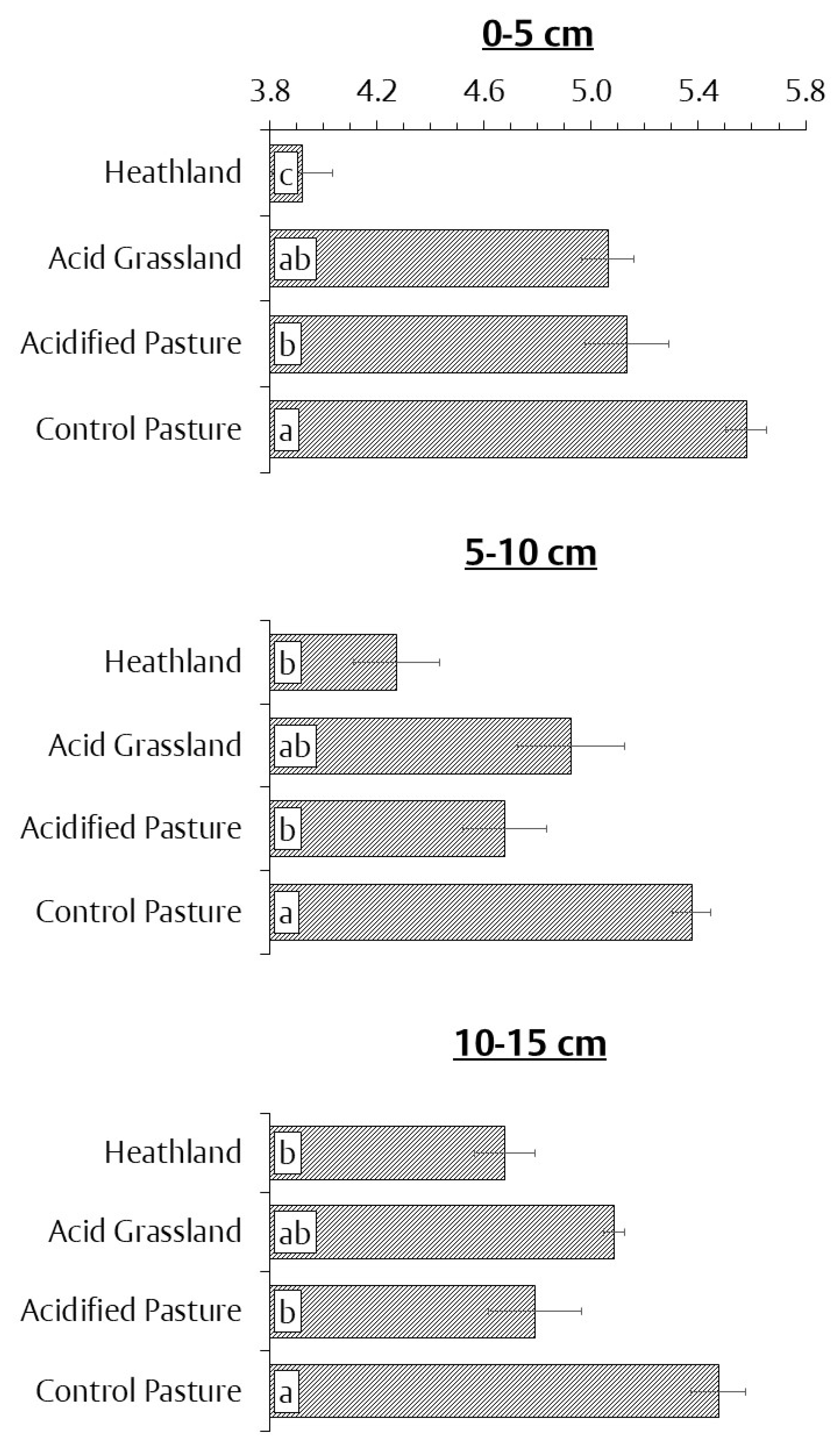
3.1. Soil pH
3.2. Plant Community
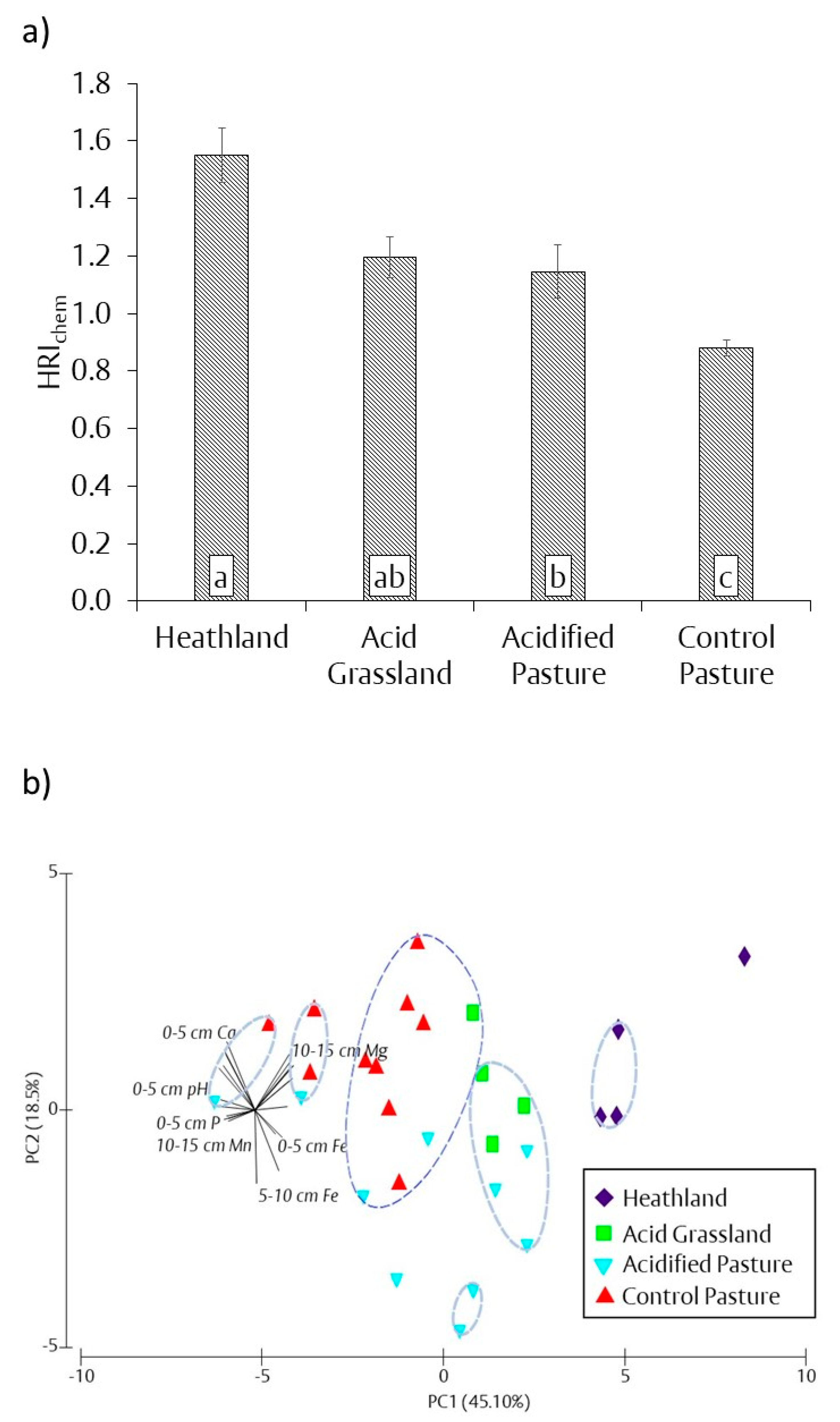
3.3. Chemical Heathland Restoration Index (HRIchem)
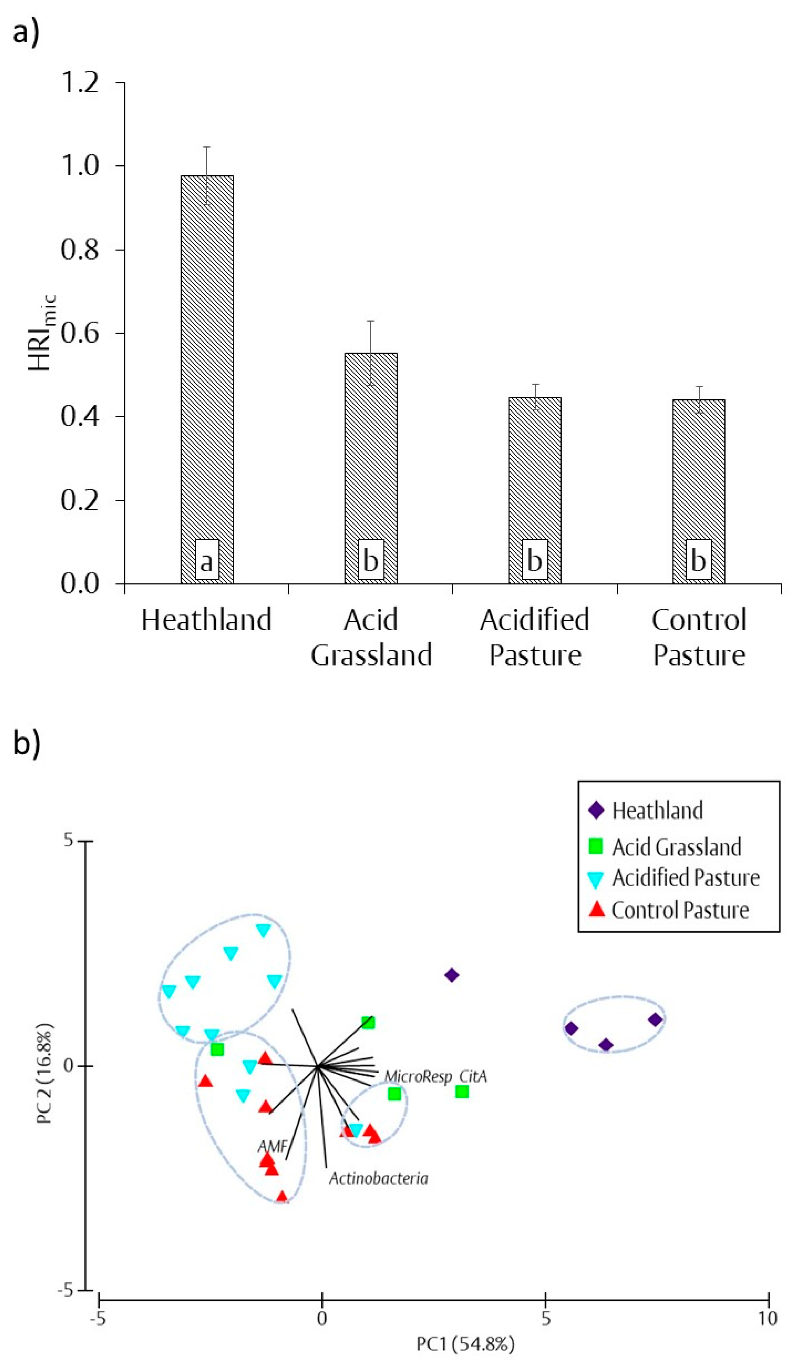
3.4. Microbial Heathland Restoration Index (HRImic)
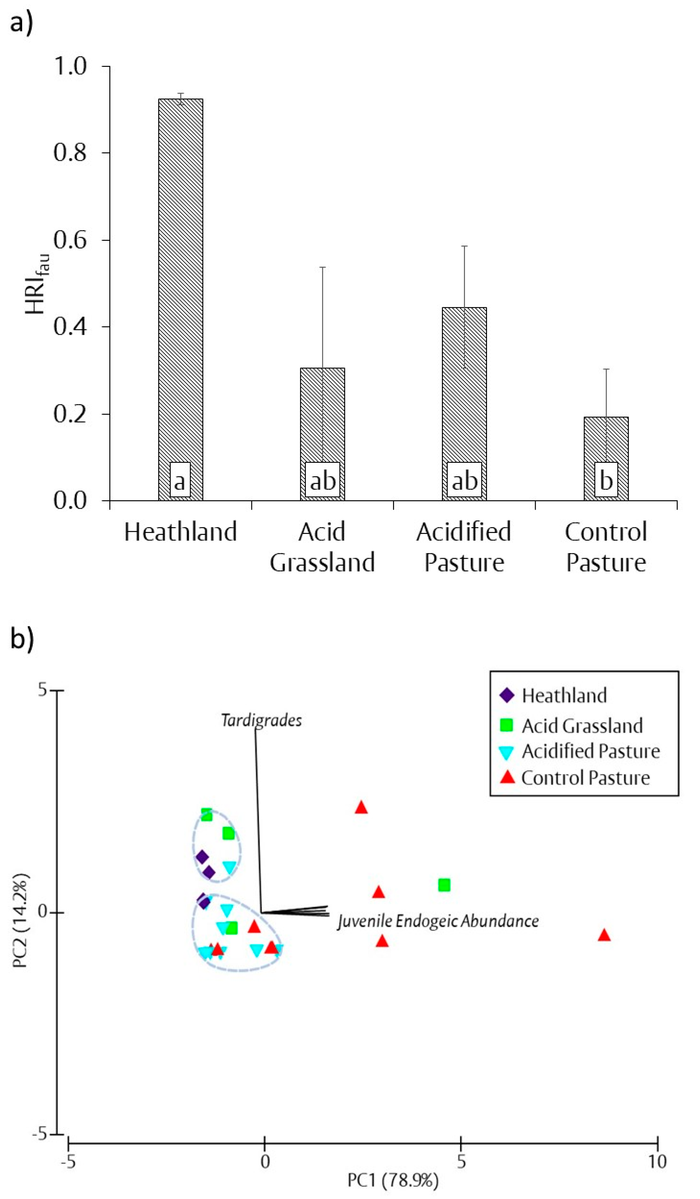
3.5. Soil Fauna Heathland Restoration Index (HRIfau)
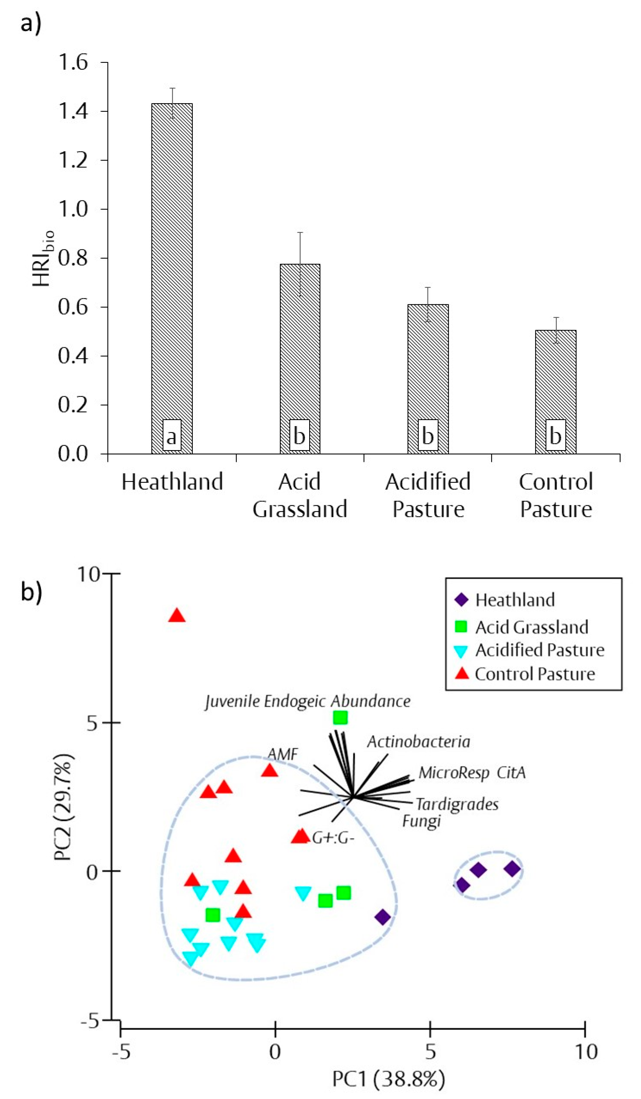
3.6. Biological Heathland Restoration Index (HRIbio)
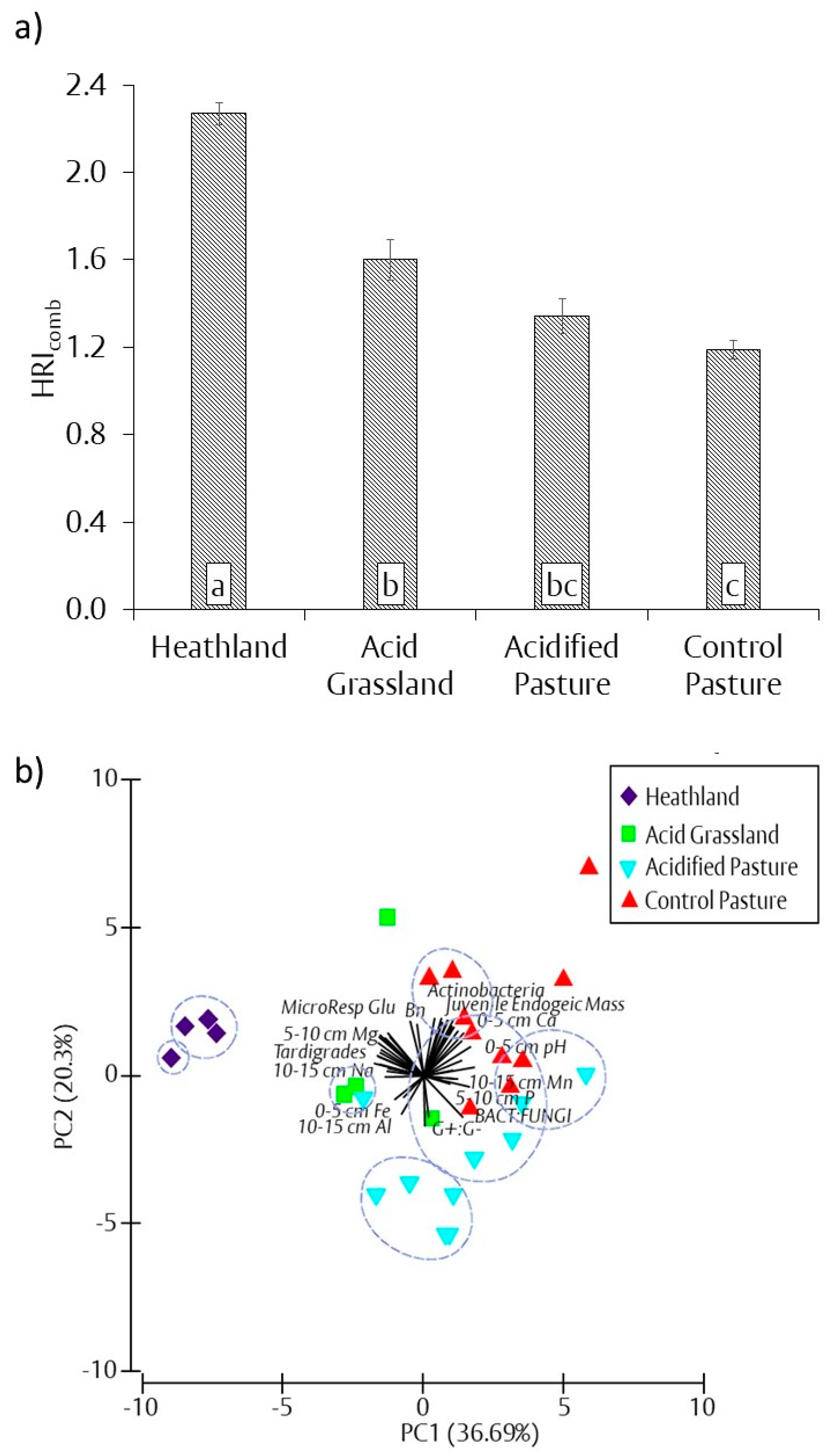
3.7. Combined Chemical and Biological Heathland Restoration Index (HRIcomb)
3.8. Data Summary
4. Discussion
4.1. Aboveground Response to Changes in Soil Chemical Properties
4.2. Belowground Response to Changes in Soil Chemical Properties
4.3. HRI Based on a Minimum Dataset and Linear Scoring System Compared to Analysis of Similarity
5. Conclusions
Author Contributions
Funding
Acknowledgments
Conflicts of Interest
References
- European Commission. Council Directive 92/43/EEC of 21 May 1992 on the conservation of natural habitats and of wild fauna and flora. Off. J. Eur. Union 1992. [CrossRef]
- HMSO. Biodiveristy: The UK Action Plan; HMSO: London, UK, 1994. [Google Scholar]
- UKBAP. UK Biodiversity Action Plan Priority Habitat Descriptions 2008 (Updated 2011); Department of Environment: London, UK, 2011. [Google Scholar]
- Clarke, C.T. Role of soils in determining sites for lowland heathland reconstruction in England. Restor. Ecol. 1997, 5, 256–264. [Google Scholar] [CrossRef]
- Newton, A.C.; Stewart, G.B.; Myers, G.; Diaz, A.; Lake, S.; Bullock, J.M.; Pullin, A.S. Impacts of grazing on lowland heathland in north-west Europe. Biol. Conserv. 2009, 142, 935–947. [Google Scholar] [CrossRef]
- Green, I.; Stockdale, J.; Tibbett, M.; Diaz, A. Heathland restoration on former agricultural land: Effects of artificial acidification on the availability and uptake of toxic metal cations. Water Air. Soil Pollut. 2007, 178, 287–295. [Google Scholar] [CrossRef]
- Mitchell, R.J.; Auld, M.H.D.; Hughes, J.M.; Marrs, R.H. Estimates of nutrient removal during heathland restoration on successional sites in Dorset, southern England. Biol. Conserv. 2000, 95, 233–246. [Google Scholar] [CrossRef]
- Farrell, M.; Healey, J.R.; Godbold, D.L.; Nason, M.A.; Tandy, S.; Jones, D.L. Modification of Fertility of Soil Materials for Restoration of Acid Grassland Habitat. Restor. Ecol. 2011, 19, 509–519. [Google Scholar] [CrossRef]
- Tibbett, M.; Diaz, A. Are sulfurous soil amendments (S0, Fe(II)SO4, Fe(III)SO4) an effective tool in the restoration of heathland and acidic grassland after four decades of rock phosphate fertilization? Restor. Ecol. 2005, 13, 83–91. [Google Scholar] [CrossRef]
- Walker, K.J.; Pywell, R.F.; Warman, E.A.; Fowbert, J.A.; Bhogal, A.; Chambers, B.J. The importance of former land use in determining successful re-creation of lowland heath in southern England. Biol. Conserv. 2004, 116, 289–303. [Google Scholar] [CrossRef]
- Kleijn, D.; Bekker, R.M.; Bobbink, R.; De Graaf, M.C.C.; Roelofs, J.G.M. In search for key biogeochemical factors affecting plant species persistence in heathland and acidic grasslands: A comparison of common and rare species. J. Appl. Ecol. 2008, 45, 680–687. [Google Scholar] [CrossRef]
- Owen, K.M.; Marrs, R.H.; Snow, C.S.R.; Evans, C.E. Soil acidification—The use of sulphur and acidic plant materials to acidify arable soils for the recreation of heathland and acidic grassland at Minsmere, UK. Biol. Conserv. 1999, 87, 105–121. [Google Scholar] [CrossRef]
- Davis, J.; Lewis, S.; Putwain, P. The re-creation of dry heathland and habitat for a nationally threatened butterfly at Prees Heath Common Reserve, Shropshire. Asp. Appl. Biol. 2011, 108, 247–254. [Google Scholar] [CrossRef]
- Lawson, C.S.; Ford, M.A.; Mitchley, J.; Warren, J.M. The establishment of heathland vegetation on ex-arable land: The response of Calluna vulgaris to soil acidification. Biol. Conserv. 2004, 116, 409–416. [Google Scholar] [CrossRef]
- Pywell, R.F.; Webb, N.R.; Putwain, P.D. Soil fertility and its implications for the restoration of heathland on farmland in Southern Britain. Biol. Conserv. 1994, 70, 169–181. [Google Scholar] [CrossRef]
- Raiesi, F. A minimum data set and soil quality index to quantify the effect of land use conversion on soil quality and degradation in native rangelands of upland arid and semiarid regions. Ecol. Indic. 2017, 75, 307–320. [Google Scholar] [CrossRef]
- Masto, R.E.; Chhonkar, P.K.; Singh, D.; Patra, A.K. Alternative soil quality indices for evaluating the effect of intensive cropping, fertilisation and manuring for 31 years in the semi-arid soils of India. Environ. Monit. Assess. 2008, 136, 419–435. [Google Scholar] [CrossRef] [PubMed]
- Romaniuk, R.; Giuffre, L.; Romero, R. A soil quality index to evaluate the vermicompost amendments effects on soil properites. J. Environ. Prot. (Irvine, Calif) 2011, 2, 502–510. [Google Scholar] [CrossRef] [Green Version]
- Biswas, S.; Hazra, G.C.; Purakayastha, T.J.; Saha, N.; Mitran, T.; Roy, S.S.; Basak, N.; Mandal, B. Establishment of critical limits of indicators and indices of soil quality in rice-rice cropping systems under different soil orders. Geoderma 2017, 292, 34–48. [Google Scholar] [CrossRef]
- Andrews, S.S.; Karlen, D.L.; Mitchell, J.P. A comparison of soil quality indexing methods for vegetable production systems in Northern California. Agric. Ecosyst. Environ. 2002, 90, 25–45. [Google Scholar] [CrossRef]
- Mukherjee, A.; Lal, R. Comparison of soil quality index using three methods. PLoS ONE 2014, 9, e105981. [Google Scholar] [CrossRef] [Green Version]
- Tibbett, M.; Gil-Martínez, M.; Fraser, T.; Green, I.D.; Duddigan, S.; De Oliveira, V.H.; Raulund-Rasmussen, K.; Sizmur, T.; Diaz, A. Long-term acidification of pH neutral grasslands affects soil biodiversity, fertility and function in a heathland restoration. Catena 2019, 180, 401–415. [Google Scholar] [CrossRef]
- Diaz, A.; Green, I.; Tibbett, M. Re-creation of heathland on improved pasture using top soil removal and sulphur amendments: Edaphic drivers and impacts on ericoid mycorrhizas. Biol. Conserv. 2008, 141, 1628–1635. [Google Scholar] [CrossRef]
- Fagúndez, J. Heathlands confronting global change: Drivers of biodiversity loss from past to future scenarios. Ann. Bot. 2013, 111, 151–172. [Google Scholar] [CrossRef] [PubMed] [Green Version]
- Pulleman, M.; Creamer, R.; Hamer, U.; Helder, J.; Pelosi, C.; Peres, G.; Rutgers, M. Soil biodiversity, biological indicators and soil ecosystem services-an overview of European approaches. Curr. Opin. Environ. Sustain. 2012, 4, 529–538. [Google Scholar] [CrossRef]
- Paz-Ferreiro, J.; Fu, S. Biological Indices for Soil Quality Evaluation: Perspectives and Limitations. Land Degrad. Dev. 2016, 27. [Google Scholar] [CrossRef]
- Menta, C. Soil Fauna Diversity—Function, Soil Degradation, Biological Indices, Soil Restoration. In Biodiversity Conservation and Utilization in A Diverse World; IntechOpen: London, UK, 2012; pp. 59–94. [Google Scholar]
- Guo, L.; Sun, Z.; Ouyang, Z.; Han, D.; Li, F. A comparison of soil quality evaluation methods for Fluvisol along the lower Yellow River. Catena 2017, 152, 135–143. [Google Scholar] [CrossRef]
- International Organization for Standardization (ISO). ISO18400-104:Soil Quality—Sampling—Part 104: Strategies; International Organization for Standardization: Geneva, Switzerland, 2018. [Google Scholar]
- Rodwell, J.S. (Ed.) Mires and Heaths. In British Plant Communities; Cambridge University Press: Cambridge, UK, 1998; Volume 2. [Google Scholar]
- Rodwell, J.S. (Ed.) Grasslands and Montane Communities. In British Plant Communities; Cambridge University Press: Cambridge, UK, 1998; Volume 3. [Google Scholar]
- Rowell, D.L. Soil Science: Methods & Applications; Taylor & Francis: London, UK, 1994. [Google Scholar]
- Stuanes, A.O.; Ogner, G.; Opem, M. Ammonium nitrate as extractant for soil exchangeable cations, exchangeable acidity and aluminum. Commun. Soil Sci. Plant Anal. 1984, 15, 773–778. [Google Scholar] [CrossRef]
- Sørensen, N.K.; Bülow-Olsen, A. Metode 14. Fosofortallet Pt. Plantedirektoratet. In Flles Arb. Jordbundsanalyser; Landbrugsministeriet: Lyngby, Denmark, 1994; pp. 1–4. [Google Scholar]
- Schloter, M.; Dilly, O.; Munch, J.C. Indicators for evaluating soil quality. Agric. Ecosyst. Environ. 2003, 98, 255–262. [Google Scholar] [CrossRef]
- Vance, E.D.; Brookes, P.C.; Jenkinson, D.S. An extraction method for measuring soil microbial biomass, C. Soil Biol. Biochem. 1987, 19, 703–707. [Google Scholar] [CrossRef]
- Brookes, P.C.; Powlson, D.S.; Jenkinson, D.S. Measurement of microbial biomass phosphorus in soil. Soil Biol. Biochem. 1982, 14, 319–329. [Google Scholar] [CrossRef]
- Hedley, M.J.; Stewart, J.W.B. Method to measure microbial phosphate in soils. Soil Biol. Biochem. 1982, 14, 377–385. [Google Scholar] [CrossRef]
- Wu, J.; Joergensen, R.G.; Pommerening, B.; Chaussod, R.; Brookes, P.C. Measurement of soil microbial biomass C by fumigation-extraction-an automated procedure. Soil Biol. Biochem. 1990, 22, 1167–1169. [Google Scholar] [CrossRef]
- Jenkinson, D.S.; Brookes, P.C.; Powlson, D.S. Measuring soil microbial biomass. Soil Biol. Biochem. 2004, 36, 5–7. [Google Scholar] [CrossRef]
- Griffiths, B.S.; Spilles, A.; Bonkowski, M. C:N:P stoichiometry and nutrient limitation of the soil microbial biomass in a grazed grassland site under experimental P limitation or excess. Ecol. Process 2012, 1, 1–11. [Google Scholar] [CrossRef] [Green Version]
- Chapman, S.J.; Campbell, C.D.; Artz, R.R.E. Assessing CLPPs using MicroResp™—A comparison with biolog and multi-SIR. J. Soils Sediments 2007, 7, 406–410. [Google Scholar] [CrossRef]
- Creamer, R.E.; Stone, D.; Berry, P.; Kuiper, I. Measuring respiration profiles of soil microbial communities across Europe using MicroResp™ method. Appl. Soil Ecol. 2016, 97, 36–43. [Google Scholar] [CrossRef]
- Campbell, C.D.; Chapman, S.J.; Cameron, C.M.; Davidson, M.S.; Potts, J.M. A rapid microtiter plate method to measure carbon dioxide evolved from carbon substrate amendments so as to determine the physiological profiles of soil microbial communities by using whole soil. Appl. Environ. Microbiol. 2003, 69, 3593–3599. [Google Scholar] [CrossRef] [Green Version]
- Bligh, E.G.; Dyer, W.J. A rapid method of total lipid extraction and purification. Can. J. Biochem. Physiol. 1959, 37, 911–917. [Google Scholar] [CrossRef] [Green Version]
- Frostegård, A.; Bååth, E. The use of phospholipid fatty acid analysis to estimate bacterial and fungal biomass in soil. Biol. Fertil. Soils 1996, 22, 59–65. [Google Scholar] [CrossRef]
- Tunlid, A.; White, D.C. Biochemical analysis of biomass, community structure, nutritional status, and metabolic activity of microbial communities in soil. In Soil Biochemistry; Stotzky, G., Bollag, J.M., Eds.; Marcel Dekker Inc.: New York, NY, USA, 1992; Volume 7, pp. 229–262. [Google Scholar]
- Bååth, E. The use of neutral lipid fatty acids to indicate the physiological conditions of soil fungi. Microb. Ecol. 2003, 45, 373–383. [Google Scholar] [CrossRef]
- Bååth, E.; Anderson, T.H. Comparison of soil fungal/bacterial ratios in a pH gradient using physiological and PLFA-based techniques. Soil Biol. Biochem. 2003, 35, 955–963. [Google Scholar] [CrossRef]
- Kaur, A.; Chaudhary, A.; Kaur, A.; Choudhary, R.; Kaushik, R. Phospholipid fatty acid—A bioindicator of environment monitoring and assessment in soil ecosystem. Curr. Sci. 2005, 89, 1103–1112. [Google Scholar]
- Zelles, L. Identification of single cultured micro-organisms based on their whole-community fatty acid profiles, using an extended extraction procedure. Chemosphere 1999, 39, 665–682. [Google Scholar] [CrossRef]
- De Deyn, G.B.; Quirk, H.; Oakley, S.; Ostle, N.; Bardgett, R.D. Rapid transfer of photosynthetic carbon through the plant-soil system in differently managed species-rich grasslands. Biogeosciences 2011, 8, 1131–1139. [Google Scholar] [CrossRef] [Green Version]
- Pankhurst, L.J.; Whitby, C.; Pawlett, M.; Larcombe, L.D.; McKew, B.; Deacon, L.J.; Morgan, S.L.; Villa, R.; Drew, G.H.; Tyrrel, S.; et al. Temporal and spatial changes in the microbial bioaerosol communities in green-waste composting. FEMS Microbiol. Ecol. 2012, 79, 229–239. [Google Scholar] [CrossRef] [PubMed] [Green Version]
- Harwood, J.L.; Russell, N.J. Lipids in Plants and Microbes; George Allen & Unwin Ltd.: London, UK, 1984. [Google Scholar]
- Zogg, G.P.; Zak, D.B.; Ringelberg, N.W.; MacDonald, N.W.; Pregitzer, K.S.; White, D.C. Compositional and functional shifts in microbial communities due to soil warming. Soil Sci. Soc. Am. J. 1997, 61, 475–481. [Google Scholar] [CrossRef] [Green Version]
- Parkes, R.J.; Taylor, J. The relationship between fatty acid distributions and bacterial respiratory types in contemporary marine sediments. Estuar. Coast. Shelf. Sci. 1983, 16. [Google Scholar] [CrossRef]
- O’Leary, W.M.; Wilkinson, S.G. Gram-positive bacteria. In Microbial Lipids; Ratledge, C., Wilkinson, S.G., Eds.; Academic Press Ltd.: London, UK, 1988; Volume 1, pp. 117–185. [Google Scholar]
- Wilkinson, S.G. Gram-negative bacteria. In Microbial Lipids; Ratledge, C., Wilkinson, S.G., Eds.; Academic Press Ltd.: London, UK, 1988; Volume 1, pp. 299–457. [Google Scholar]
- Olsson, P.A. Signature fatty acids provide tools for determination of the distribution and interaction of mycorrhizal fungi. FEMS Microbiol. Ecol. 1999, 29, 303–310. [Google Scholar] [CrossRef]
- Federle, T.W. Microbial distribution in soil—New techniques. In Perspectives in Microbial Ecology; Megusar, F., Gantar, M., Eds.; Slovene Society for Microbiology: Ljubljana, Slovenia, 1986; pp. 493–498. [Google Scholar]
- Vestal, J.R.; White, D.C. Lipid analysis in microbial ecology: Quantitative approaches to the study of microbial communities. Biogeoscience 1989, 39, 535–541. [Google Scholar] [CrossRef]
- Frostegard, A.; Tunlid, A.; Baath, E. Phospholipid fatty acid composition, biomass, and activity of microbial communities from two soil types experimentally exposed to different heavy metals. Appl. Environ. Microbiol. 1993, 59, 3605–3617. [Google Scholar] [CrossRef] [Green Version]
- Pankhurst, C.E.; Yu, S.; Hawke, B.G.; Harch, B.D. Capacity of fatty acid profiles and substrate utilization patterns to describe differences in soil microbial communities associated with increased salinity or alkalinity at three locations in South Australia. Biol. Fertil. Soils 2001, 33, 204–217. [Google Scholar] [CrossRef]
- Lechevalier, M.P. Lipids in bacterial taxonomy: A taxonomists view. Crit. Rev. Microbiol. 1977, 5, 109–210. [Google Scholar] [CrossRef] [PubMed]
- Kroppenstedt, R.M. Fatty acid and menaquinone analysis of actinomycetes and related organisms. In Chemical Methods Bacteria System; Goodfellow, M., Minnikin, D.E., Eds.; Elsevier Science & Technology Books: London, UK, 1985; pp. 173–199. [Google Scholar]
- Sherlock, E. Key to the Earthworms of Britain and Ireland; Field Studies Council: Shrewsbury, UK, 2012. [Google Scholar]
- Yeates, G.W. Nematodes as soil indicators: Functional and biodiversity aspects. Biol. Fertil. Soils 2003, 37, 199–210. [Google Scholar] [CrossRef]
- Yeates, G.W.; Bongers, T.; De Goede, R.G.M.; Freckman, D.W.; Georgieva, S.S. Feeding Habits in Soil Nematode Families and Genera-An Outline for Soil Ecologists. J. Nematol. 1993, 25, 315–331. [Google Scholar] [PubMed]
- Riesch, F.; Stroh, H.G.; Tonn, B.; Isselstein, J. Soil pH and phosphorus drive species composition and richness in semi-natural heathlands and grasslands unaffected by twentieth-century agricultural intensification. Plant Ecol. Divers. 2018, 11, 239–253. [Google Scholar] [CrossRef]
- Manning, P.; Putwain, P.D.; Webb, N.R. The role of soil phosphorus sorption characteristics in the functioning and stability of lowland heath ecosystems. Biogeochemistry 2006, 81, 205–217. [Google Scholar] [CrossRef]
- Green, I.; Evans, D.; Diaz, A. Modifying soil chemistry to enhance heathland recreation: A use for sulphur captured during oil refining. Int. J. Plant Soil Sci. 2015, 6, 272–282. [Google Scholar] [CrossRef] [Green Version]
- Owen, K.M.; Marrs, R.H. The use of mixtures of sulfur and bracken litter to reduce pH of former arable soils and control ruderal species. Restor. Ecol. 2001, 9, 397–409. [Google Scholar] [CrossRef]
- Roem, W.J.; Klees, H.; Berendse, F. Effects of nutrient addition and acidification on plant species diversity and seed germination in heathland. J. Appl. Ecol. 2002, 39, 937–948. [Google Scholar] [CrossRef]
- Harris, J. Soil microbial communities and restoration ecology: Facilitators or followers? Science 2009, 325, 573–574. [Google Scholar] [CrossRef]
- Vogels, J.J.; Verberk, W.C.E.P.; Lamers, L.P.M.; Siepel, H. Can changes in soil biochemistry and plant stoichiometry explain loss of animal diversity of heathlands? Biol. Conserv. 2017, 212, 432–447. [Google Scholar] [CrossRef]
- Radujković, D.; van Diggelen, R.; Bobbink, R.; Weijters, M.; Harris, J.; Pawlett, M.; Vicca, S.; Verbruggen, E. Initial soil community drives heathland fungal community trajectory over multiple years through altered plant–soil interactions. New Phytol. 2020, 225, 2140–2151. [Google Scholar] [CrossRef] [PubMed]
- De Graaf, M.C.C.; Verbeek, P.J.M.; Bobbink, R.; Roelofs, J.G.M. Restoration of species-rich dry heaths: The importance of appropriate soil conditions. Acta. Bot. Neerl. 1998, 47, 89–111. [Google Scholar]
- Hart, S.C.; DeLuca, T.H.; Newman, G.S.; MacKenzie, M.D.; Boyle, S.I. Post-fire vegetative dynamics as drivers of microbial community structure and function in forest soils. For. Ecol. Manag. 2005, 220, 166–184. [Google Scholar] [CrossRef]
- Orozco-Aceves, M.; Standish, R.J.; Tibbett, M. Soil conditioning and plant-soil feedbacks in a modified forest ecosystem are soil-context dependent. Plant Soil 2015, 390, 183–194. [Google Scholar] [CrossRef]
- Orozco-Aceves, M.; Standish, R.J.; Tibbett, M. Long-term conditioning of soil by plantation eucalypts and pines does not affect growth of the native jarrah tree. For. Ecol. Manag. 2015, 338, 92–99. [Google Scholar] [CrossRef]
- Van der Bij, A.U.; Weijters, M.J.; Bobbink, R.; Harris, J.A.; Pawlett, M.; Ritz, K. Facilitating ecosystem assembly: Plant-soil interactions as a restoration tool. Biol. Conserv. 2018, 220, 272–279. [Google Scholar] [CrossRef]
- Kardol, P.; Wardle, D.A. How understanding aboveground-belowground linkages can assist restoration ecology. Trends Ecol. Evol. 2010, 25, 670–679. [Google Scholar] [CrossRef]
- Lane, M.; Hanley, M.E.; Lunt, P.; Knight, M.E.; Braungardt, C.B.; Ellis, J.S. Chronosequence of former kaolinite open cast mines suggests active intervention is required for the restoration of Atlantic heathland. Restor. Ecol. 2020, 28, 661–667. [Google Scholar] [CrossRef]


| Microbial Group | Signature PLFAs or Biomarkers | References |
|---|---|---|
| Total bacteria | 15:0, 15:0i, 15:0ai, 16:0i, 17:0i, 17:0ai, 16:1 ω7c, 17:0c, 19:0c | [47,54,55] |
| Gram-positive bacteria | 15:0i, 15:0ai, 16:0i, 17:0i, 17:0ai | [56,57] |
| Gram-negative bacteria | 16:1ω7c, 17:0c, 19:0c | [51,58] |
| Arbuscular mycorrhizal fungi | 16:1ω5 | [59] |
| Ectomycorrhizal fungi | 18:2ω6,9 | [46,59,60,61,62,63] |
| Actinobacteria | 18:0 (10Me) | [64,65] |
| Chemical HRI (HRIchem) | Soil Micro- and Macrofauna HRI (HRIfau) | Soil Microbes HRI (HRImic) | Biological HRI (HRIbio) | Combined HRI (HRIcomb) |
|---|---|---|---|---|
| 0-5 cm: Al; Ca; Fe; K; | Earthworm Abundance and Mass: | Total Bacteria Abundance | All variables listed in HRIfau and HRImic | All variables listed in HRIchem and HRIbio |
| Mg; Mn; Na; | Total (juvenile and adult; all ecological groups) | G+:G- | together | together |
| P; pH | Adult (all ecological groups) | Total Actinobacteria Abundance | ||
| Juvenile (all ecological groups) | Total Fungi Abundance | 34 Variables | 58 variables | |
| 5-10 cm: Al; Ca; Fe; K; | Total epigeic (juvenile and adult) | Total Arbuscular Mycorrhizal Fungi Abundance | ||
| Mg; Mn; Na; | Adult epigeic | Bacteria:Fungi | 7 Variables in minimum dataset: | 15 variables in the minimum dataset |
| P; pH | Juvenile epigeic | Microbial Biomass C, N and P | ||
| Total endogeic (juvenile and adult) | Gram positive bacteria: Gram negative bacteria ratio (G+:G-) | G+:G | ||
| 10-15 cm: Al; Ca; Fe; | Adult endogeic | Microbial Respiration (MicroResp™) | Total Actinobacteria abundance | Total Actinobacteria abundance |
| K; Mg; Mn; | Juvenile endogeic | α-Ketoglutaric acid | Total Fungi Abundance | Bacteria:Fungi |
| Na; P; pH | Total anecic (juvenile and adult) | L-Alanine | Total Arbuscular Mycorrhizal Fungi | Microresp α-D-Glucose |
| Adult anecic | Citric acid | Microresp Citric Acid | Microbial Biomass N | |
| Juvenile anecic | ɣ-Aminobutyric acid | Juvenile Endogeic Abundance | Juvenile Endogeic Mass | |
| 24 Variables | Nematode Abundance: | α-D-Glucose | Total Tardigrade Abundance | Total Tardigrade Abundance |
| Total (all functional groups) | L-Malic acid | 0–5 cm pH | ||
| 7 * Variables in | Plant Parasite | Water | 0–5 cm Ca | |
| minimum dataset | Bacterial Feeder | 0–5 cm Fe | ||
| Fungal Feeder | 14 Variables | 5–10 cm Mg | ||
| Predator | 5–10 cm P | |||
| Omnivore | 3 * Variables in minimum dataset | 10–15 cm Al | ||
| Total Rotifer Abundance | 10–15 cm Mn | |||
| Total Tardigrade Abundance | 10–15 cm Na | |||
| 24 Variables | ||||
| 2 * Variables in minimum dataset |
| ANOSIM Pair-Wise Test p-Value | |||
|---|---|---|---|
| Heathland | Acid Grassland | Acidified Pasture | |
| Heathland | - | - | - |
| Acid Grassland | 0.029 | - | - |
| Acidified Pasture | 0.004 | 0.378 | - |
| Control Pasture | 0.002 | 0.021 | 0.002 |
| ANOSIM Pair-Wise Test p-Value | |||
|---|---|---|---|
| Heathland | Acid Grassland | Acidified Pasture | |
| Heathland | - | - | - |
| Acid Grassland | 0.057 | - | - |
| Acidified Pasture | 0.003 | 0.013 | - |
| Control Pasture | 0.001 | 0.004 | 0.002 |
| ANOSIM Pair-Wise Test p-Value | |||
|---|---|---|---|
| Heathland | Acid Grassland | Acidified Pasture | |
| Heathland | - | - | - |
| Acid Grassland | 0.086 | - | - |
| Acidified Pasture | 0.068 | 0.016 | - |
| Control Pasture | 0.243 | 0.229 | 0.017 |
| ANOSIM Pair-Wise Test p-Value | |||
|---|---|---|---|
| Heathland | Acid Grassland | Acidified Pasture | |
| Heathland | - | - | - |
| Acid Grassland | 0.057 | - | - |
| Acidified Pasture | 0.001 | 0.006 | - |
| Control Pasture | 0.003 | 0.084 | 0.001 |
| ANOSIM Pair-Wise Test p-Value | |||
|---|---|---|---|
| Heathland | Acid Grassland | Acidified Pasture | |
| Heathland | - | - | - |
| Acid Grassland | 0.029 | - | - |
| Acidified Pasture | 0.001 | 0.048 | - |
| Control Pasture | 0.001 | 0.060 | 0.001 |
 resulted in a significant difference in treatments according to one-way ANOVA and Tukey’s post hoc testing (p < 0.05). See part a of Figure 3, Figure 4, Figure 5, Figure 6 and Figure 7 for full results. ** Analysis of similarity pair-wise comparisons marked with a
  resulted in a significant difference in treatments based on Euclidean matrix of similarity (p < 0.05).
resulted in a significant difference in treatments according to one-way ANOVA and Tukey’s post hoc testing (p < 0.05). See part a of Figure 3, Figure 4, Figure 5, Figure 6 and Figure 7 for full results. ** Analysis of similarity pair-wise comparisons marked with a resulted in a significant difference in treatments based on Euclidean matrix of similarity (p < 0.05).
resulted in a significant difference in treatments based on Euclidean matrix of similarity (p < 0.05).
resulted in a significant difference in treatments according to one-way ANOVA and Tukey’s post hoc testing (p < 0.05). See part a of Figure 3, Figure 4, Figure 5, Figure 6 and Figure 7 for full results. ** Analysis of similarity pair-wise comparisons marked with a resulted in a significant difference in treatments based on Euclidean matrix of similarity (p < 0.05).Significant Difference in Pair-wise Comparison? (  if p < 0.05) if p < 0.05) | ||||
|---|---|---|---|---|
| Heathland Restoration Index * | Analysis of Similarity ** | |||
| Acidified Pasture vs. Control Pasture | HRIchem |  | ANOSIMchem |  |
| HRImic | ANOSIMmic |  | ||
| HRIfau | ANOSIMfau |  | ||
| HRIbio | ANOSIMbio |  | ||
| HRIcomb | ANOSIMcomb |  | ||
| Acidified Pasture vs. Heathland | HRIchem |  | ANOSIMchem |  |
| HRImic |  | ANOSIMmic |  | |
| HRIfau | ANOSIMfau | |||
| HRIbio |  | ANOSIMbio |  | |
| HRIcomb |  | ANOSIMcomb |  | |
© 2020 by the authors. Licensee MDPI, Basel, Switzerland. This article is an open access article distributed under the terms and conditions of the Creative Commons Attribution (CC BY) license (http://creativecommons.org/licenses/by/4.0/).
Share and Cite
Duddigan, S.; Gil-Martínez, M.; Fraser, T.; Green, I.; Diaz, A.; Sizmur, T.; Pawlett, M.; Raulund-Rasmussen, K.; Tibbett, M. Evaluating Heathland Restoration Belowground Using Different Quality Indices of Soil Chemical and Biological Properties. Agronomy 2020, 10, 1140. https://doi.org/10.3390/agronomy10081140
Duddigan S, Gil-Martínez M, Fraser T, Green I, Diaz A, Sizmur T, Pawlett M, Raulund-Rasmussen K, Tibbett M. Evaluating Heathland Restoration Belowground Using Different Quality Indices of Soil Chemical and Biological Properties. Agronomy. 2020; 10(8):1140. https://doi.org/10.3390/agronomy10081140
Chicago/Turabian StyleDuddigan, Sarah, Marta Gil-Martínez, Tandra Fraser, Iain Green, Anita Diaz, Tom Sizmur, Mark Pawlett, Karsten Raulund-Rasmussen, and Mark Tibbett. 2020. "Evaluating Heathland Restoration Belowground Using Different Quality Indices of Soil Chemical and Biological Properties" Agronomy 10, no. 8: 1140. https://doi.org/10.3390/agronomy10081140