Evaluation of In-Season Management Zones from High-Resolution Soil and Plant Sensors

Abstract

The adoption of precision agriculture has the potential to increase the environmental sustainability of cropping systems as well as farmers’ income. Farmers in transition to precision agriculture need low-input and effective protocols to delineate homogenous management zones to optimize their actions without past knowledge e.g., yield maps. Different approaches have been developed so far, based on the analysis of the within-field variability in crop and soil properties, but procedures were rarely suited for operational conditions. We identified here a low-inputs protocol to map management zones from soil electrical conductivity and/or crop vegetation indices, using a winter wheat field in northern Italy as a pilot case. The reliability of the alternative data sources was evaluated at three crop development stages using a yield map as reference. Red-edge and NIR (NDRE) bands were the most reliable data sources for management zones identification, with 62%, 68%, and 74% of correct classifications at early tillering, stem elongation, and late booting, respectively. Our work identifies a minimum dataset for accurate management zones’ definition and highlights that in-season monitoring based on the red-edge band was able to reliably identify management zones already at early tillering, despite minor differences in crop growth.

1. Introduction

The intensification of agricultural systems led to the excessive use of irrigation water, fertilizers, and other agrochemicals, with detrimental effects on environmental sustainability and farmers’ profitability [1]. Standard management practices in conventional agriculture entail consistent application of water and agrochemicals, disregarding the within-field variability of crop status and needs [2]. Precision agriculture (PA) aims at improving the resources use efficiency to maximize yield and reduce production costs, through the optimization of the timing and the supply of agrochemicals [3]. The assessment of the within-field variability of soil and vegetation properties is the basis of PA because it allows modulating farmer inputs release according to the actual crop requirements [2]. A key concept in PA is the variable-rate application, based either on application maps or on real-time sensors [4]. Examples of the latter are tractor-mounted data acquisition and processing systems used to optimize nitrogen fertilization [5,6] and weed management [7].

Map-based techniques are used to define management zones (MZs) characterized by homogeneous yield-limiting factors [8], allowing a site-specific application of agrochemicals [9]. The first methodology used in MZs definition consisted of manual samplings to determine soil properties and crop yield [9,10,11]. This approach was replaced by proximal sensors to measure apparent soil electrical conductivity (ECa), a proxy of multiple physical and chemical soil properties [12]. Then, the multispectral response of vegetation acquired by satellites or by aerial vehicles has been progressively adopted in MZs definition [8]. After the soil and/or crop sensing has been performed, statistical analyses are used [13] to integrate soil properties and spectral crop data [8,14,15]. The most used statistical methods are k-means clustering, fuzzy clustering, neural network models, classification trees, and principal components analysis [16,17]. All these methods have been used with different input variables, including soil and crop properties [18] as well as crop yield [19], without any reference approach or data source widely recognized [20]. Moreover, the timing of field surveys and the number of MZs are often set according to the specific MZs mapping method, rather than driven by agronomic indications [17]. Therefore, there is the need of identifying effective and low-input procedures for MZs mapping among the plethora of existing methodologies and data sources, especially in contexts where farmers are transitioning to precision agriculture, with no ex ante knowledge of the within-field variability. This is the case of wheat systems in northern Italy, where the adoption of precision agriculture has just begun despite its possible benefits in safeguarding environmental suitability while maximizing crop yields.

This study aims at defining a low-input methodology for MZs mapping based on high-resolution soil and crop sensors (EMI sensor and airborne digital camera), which can be adopted by farmers in the first year of adoption of precision agriculture when yield maps are not available. Alternative sources of information recorded during the wheat growing season were evaluated by multivariate data analysis and then used for MZs mapping. The resulting maps were analyzed to identify the most useful period and data source for the field survey to optimize wheat management. The performances of the different methods of MZs mapping were evaluated according to their accuracy, reliability, and discrimination ability in reproducing actual yield. The agronomic meaning of the resulting MZs was finally validated via an experimental trial set up to study the crop response to different nitrogen levels in each MZ.

2. Materials and Methods

Figure 1 shows the workflow of our study, which is articulated in three steps: soil, vegetation, and yield data acquisition and processing (Section 2.2), and data analysis, where (i) multivariate analysis of the different sources was performed, (ii) MZs map derived by different data sources were evaluated, and (iii) the experimental field data were analyzed (Section 2.3).

A soil survey was performed before winter wheat sowing with an electromagnetic multi-frequency electromagnetic induction (EMI) sensor to measure soil electrical conductivity, considered as a proxy for texture and organic matter (Section 2.2.1). Then, vegetation monitoring has been carried out in three wheat development stages (early tillering, BBCH 25; beginning of stem elongation, BBCH 31; late booting stage, BBCH 45) [21], using a multispectral camera mounted on a unmanned aerial vehicle (UAV), and simple and multi-temporal vegetation indices were calculated (Section 2.2.2). At harvest, a yield map was acquired (Section 2.2.4) and used as a reference to evaluate the accuracy of the alternative sources for MZs mapping.

Multivariate analysis was performed to highlight the contribution of soil and vegetation data on MZs definition (Section 2.3.1) and to select the best predictors of yield. Then, alternative MZs were drawn via k-means fuzzy clustering (Section 2.3.2). These maps were compared with the reference yield map via contingency tables (Section 2.3.3).

In order to evaluate the agronomical value of the identified MZs, a field trial (Section 2.3.4) was carried out (Section 2.2.3), to study the impact of MZs together with nitrogen fertilization levels on crop growth.

2.1. Site Description and Crop Management

The MZs mapping was performed in a winter wheat (Triticum aestivum, var. Basmati) field of 11.3 ha located in Sant’Angelo Lodigiano (Lodi), Italy (45°13’19.6644’’ N, 9°25’42.7548’’ E, altitude 73 m asl) at Cascina Belfuggito, owned by Morando Bolognini Foundation. Wheat was sown on 10th November 2015, fertilizations were performed on 13th February 2016 (ammonium nitrate, 52 kg N ha⁻¹), and on 18th March 2016 (urea, 92 kg N ha⁻¹); wheat was harvested on 28th June 2016.

Minimum and maximum daily air temperatures in 2015–2016 growing season were in line with the climatic norm (1993–2016, Figure S1), and were not limiting for wheat development. Precipitations in the early crop establishment phase were lower than the average (November–January: 29 mm vs. 213 mm), whereas February, May, and June were characterized by larger precipitations than the averages (145, 121, and 71 mm vs. 51, 77, and 54 mm), leading to cumulated values similar to the climatic norm (441 mm vs. 523 mm) (Figure S2).

2.2. In-Season Data Acquisition and Processing

2.2.1. Soil Monitoring and Mapping

The geophysical sensor Profiler EMP400 (Geophysical Survey Systems, Inc., Nashua, NH, USA) was used to measure soil properties. This sensor is based on electromagnetic induction. It measures ECa at a frequency ranging from 1 to 16 kHz, to explore increasing soil depths. The ECa measurements taken at 15 kHz were considered here, with a vertical orientation of dipoles, corresponding to about 1 m of soil depth of exploration, according to maximum root depth of winter wheat. The survey was carried out at the end of January 2016, when the soil water content was close to field capacity.

The ECa measurements were interpolated by ordinary kriging (Figure S4) using the software GStat [22]. The experimental variogram was calculated, and the parameters of the variogram model were selected and validated. All the ECa data were interpolated on a 1 m grid, then resampled at 5 m to allow comparing soil MZs maps with the other maps.

2.2.2. Monitoring and Mapping the Within-Field Crop Variability

Two surveys were carried out with a multispectral camera (MicaSense RedEdge digital camera; MicaSense, Inc., Seattle, WA, USA) mounted on a UAV to acquire crop data to characterize the crop spatial variability. The multispectral camera acquires reflectance in five discrete bands: blue band (B), centered at 475 nm; green band (G), centered at 560 nm; red band (R), centered at 668 nm; red-edge band (RE), centered at 717 nm; near-infrared band (NIR), centered at 840 nm. The camera was mounted on a coaxial octocopter UAV platform, with a maximum take-off mass of 12 kg and equipped with a GNSS (Global Navigation Satellite System) NEO-M8N (u-blox, Thalwil, Switzerland).

Image acquisition was carried out in three wheat development stages: early tillering (eTl), beginning of stem elongation (StEl), and late boot stage (lB). The field surveys were performed at 120 m altitude at low flight speed (8 m s⁻¹). The flight plan guaranteed 80% of forward and sideward overlapped, as needed for the mosaicking process. Before and after each flight, images of a white reference panel of known reflectance were acquired, allowing the radiometric calibration of the images collected by the camera. All the images were uploaded to the MicaSense Atlas cloud, a service for data pre-processing and production of orthoimage, i.e., a geo-referenced single 5-band 16-bit image containing the reflectance values expressed as digital numbers. The orthoimage had a spatial resolution of 8.23 cm, then it was resampled at 5 m grid using the QGIS software (version 3.4, Madeira). The grid dimension of 5 m, was chosen as a compromise between the very high resolution of the digital cameras used and the operative grid of agricultural machinery used for field operations. Moreover, the 5 m grid allowed processing data in a time suitable for operational condition.

Different normalized difference vegetation indices (

Table 1. Definition, acronyms, and equations of the vegetation indices used in the study. Cumulative vegetation index (cumVI) was calculated for each vegetation index present in the table (VI) at three wheat development stages (1 = early tillering, 2 = stem elongation, and 3 = late booting).

Definition	Vegetation Index	Equation
Normalized difference vegetation index	NDVI	(NIR−R)/(NIR+R)
Green normalized difference vegetation index	GNDVI	(NIR−G)/(NIR+G)
Normalized difference red-edge	NDRE	(NIR−B)/(NIR+B)
Cumulative vegetation index	cumVI	$\sqrt{{\mathrm{VI}}_1^2+{\mathrm{VI}}_2^2+{\mathrm{VI}}_3^2}$

) were calculated using QGIS software (version 3.4, Madeira) from the multispectral data, to obtain the vegetation maps used for MZs definition. Three indices were considered: the normalized difference vegetation index (NDVI), the green normalized difference vegetation index (GNDVI), and the normalized difference red-edge index (NDRE). The NDVI is the most widely used index to map crop vigor. The GNDVI and NDRE are known to better reflect the leaf chlorophyll content than NDVI, which is more affected by canopy structural changes. Finally, the cumulative vegetation indices [23] were calculated to test the impact of subsequent surveys on MZs mapping performances.

2.2.3. Monitoring Crop Growth Conditions: Crop Response to Nitrogen

Crop response to N fertilization was evaluated in three zones within the field (Figure S3), by setting up a completely randomized block design with three replicates and three fertilization levels (0, 72, and 144 kg ha⁻¹, identified as N0, N1, and N2, respectively). The three zones were selected according to the preliminary analysis of soil ECa map (Figure S4) and visual assessment of Google aerial images. Fertilizers were hand-spread on the experimental plots (5 × 7 m): 36% of the total rate was applied as ammonium nitrate on 13th February 2016 (BBCH 23) and the remaining 64% was applied as urea on 18th March 2016 (BBCH 25). Wheat plants grown in 0.5 m² were cut above the collar in correspondence to the UAV-surveys and at harvest, to determine aboveground biomass (AGB) dry matter (DM) (t DM ha⁻¹) and N uptake (kg N ha⁻¹). The samples were oven-dried at 105 °C to determine dry weight and ground with a rotary-knife mill equipped with a sieve of 4 mm mesh; subsequently, a part was ground with a ZM 100 centrifugal mill equipped with a sieve of 0.2 mm mesh (Retsch Gmbh & Co., Haan, Germany). The total N of samples was determined by dry combustion using ThermoQuest NA1500 elemental analyzer (Carlo Erba).

2.2.4. Yield Monitoring

The crop was harvested on 28th June 2016 with a Claas Lexion 570 (CLAAS KGaA mbH, Harsewinkel, Germany) harvester equipped with sensors for yield mapping. Harvested grains were collected in a wagon and weighted, to correct the yield data acquired through the harvester.

The yield map consisted of a data layer containing the geographical coordinates of points and the associated yield measurements from the harvester sensor. The vector of points was transformed into a vector of polygons by the Voronoi tessellation implemented in QGIS, and the resulting map was then resampled at a 5 m grid.

2.3. Data Analysis

2.3.1. Multivariate Data Analysis

Principal component analysis (PCA) was performed to identify patterns of similarity in the spatial variability of soil and crop data and to identify the most meaningful source of information. The input variables of PCA were the five bands recorded at each UAV flight (B, R, G, RE, and NIR bands) and the ECa values all with the same weight; yield data, development stages, and Y-MZs were not used to compute principal components (PCs) but their coordinates in the PCs space were calculated after the analysis (supplementary variables). An agglomerative hierarchical clustering on PCs was then performed (Euclidean metrics and Ward’s minimum variance method were set to build the tree). Each cluster was described by the mean values of the original variables (ECa, B, R, RE, and NIR bands). Moreover, each cluster was qualitatively described taking into account both spatial and temporal variability, i.e., labeling pixels depending on wheat development stages and the three yield-based MZs (low, medium, and high productivity). For each supplementary variable, a v-test was calculated to quantify its presence in the clusters [24]. The sign of the v-statistic indicated over- and under-representation (positive and negative, respectively) of the category in the cluster. The PCA and hierarchical clustering on PCs were performed using FactoMineR R package [24] in R 3.6.2 environment [25].

2.3.2. Management Zones Definition

Management zone analyst software [26] was used to perform k-means fuzzy clustering to identify MZs. The k-means algorithm is based on the minimization of the sum of squared Euclidean distances of all data points from the cluster barycenter, through an iterative process that assigns data points to clusters until a minimum error is reached. The following clustering parameters were specified: maximum number of iterations = 300, convergence criterion = 0.0001, minimum number of clusters = 2, maximum number of clusters = 4. Fuzzy k-means further uses a weighting exponent to control partial memberships to the cluster, which was set to 1.3 [27]. The optimal number of classes was chosen according to the default method from the software. The results of MZA clustering were the predictor-based MZs maps, based on soil or crop properties: ECa-based MZs, indicated as soil-MZ; NDVI-, NDRE-, and GNDVI-based MZs in the three development stages, indicated as [VI]-MZ, where VI is the vegetation index (e.g., NDVI-MZs). The yield-based MZs map (Y-MZs) was produced by MZA clustering and considered as the reference map.

2.3.3. Site-Specific Accuracy Assessment of the Delineated MZs

The similarity of each predictor-based MZs map with the Y-MZs map was evaluated via contingency tables [28]. Two statistics were calculated: the proportion of correct classification (PCC), i.e., the number of grid cells correctly assigned to the different MZs divided by the total number of cells, and the Heidke skill scores (HSS), which measures the accuracy of the classification without considering the fraction of cells which would be correctly classified due to random chance (Equation (1)) [28]:

$$HSS=\frac{{\sum }_{i=1}^{I}p(prM{Z}_i,yM{Z}_{i)-}{\sum }_{i=1}^{I}p\left(prM{Z}_i\right)p\left(yM{Z}_i\right)}{1-{\sum }_{i=1}^{I}p\left(prM{Z}_i\right)p\left(yM{Z}_i\right)}\times 100,$$

(1)

where p(prMZ_i, yMZ_i) is the joint distribution of predictor-based MZs and Y-MZs, p(prMZ_i) is the marginal distribution of predictor-based MZs classification, and p(yMZ_i) is the marginal distribution of Y-MZs classification, for each of the I couples of predictor-based MZs and yield-based MZs classes.

Each multi-category contingency table, resulting from the comparison between the different MZs maps and Y-MZs, was reduced to dichotomous tables (Figure 2).

Six statistics for each MZs map were calculated from the dichotomous tables (for the definition of a, b, c, d, refer to Figure 2): (1) Critical success index (CSI = a/(a + b + c), with optimum at 1), the proportion of correct classifications after removing incorrect classifications; (2) Bias (BIAS = (a + b)/(a + c), with optimum at 1), the ratio of the predictor-based MZ_i and the Y-MZ_i; (3) False alarm ratio (FAR = b/(a + b), with optimum at 0), the proportion of predictor-based MZ_i that did not correspond to the same Y-MZi; (4) Probability of false detection (F = b/(b + d), with optimum at 0), the ratio of false alarms in reproducing Y-MZ_i; (5) Hit rate (H = a/(a + c), with optimum at 1), the ratio of correctly classified MZ; (6) Proportion of correct classification (PCC = (a + d)/(a + b + c + d), with optimum at 1). The contingency tables were analyzed with MATLAB (version 2014b; MathWorks, Natick, MA, USA).

2.3.4. Agronomic Evaluation

The accompany plot trial was designed in order to understand the causes of variability of crop growth and yield in the MZs during the whole growing season. The effects of the zone and N fertilization on wheat yield and N uptake were assessed by a split-plot ANOVA model. The between-subject factor “zone” was considered fixed with three levels (correspondent to the yield-based Y-MZ1, Y-MZ2, and Y-MZ3); subjects (blocks) within each zone were random, and the within-subject factor “N fertilizer” was fixed with three levels (0, 72, and 144 kg N ha⁻¹). Planned orthogonal contrasts were used to assess the linear and quadratic trends in AGB and N uptake in response to N fertilizer and to assess the differences between zones (zone 1 vs. zone 2 and 3, and zone 2 vs. zone 3) as well as the interaction between factors. ANOVA was executed with the GLM procedure in SPSS Version 26.0.0.1 (IBM Inc., Armonk, NY; contrasts were calculated with the LMATRIX and MMATRIX commands. The effects of factors and their interactions were considered significant at p = 0.05.

3. Results

3.1. Multivariate Data Analysis

The results of PCA and hierarchical clustering applied to the principal components are shown in Figure 3.

The first two principal components (PC) accounted for 83% of the total variance and were selected to summarize the data. The PC1 explained 63% of the total variance and had a strong positive correlation with B, G, R, RE bands (r > 0.95, p < 0.05). As shown in Figure 3b, spectral crop properties at eTl and StEl were similar, whereas at lB, generally higher reflectance in the five bands was recorded. The second principal component (PC2) explained 20% of the total variance and was positively correlated with NIR (r = 0.78, p < 0.05) and with ECa (r = 0.60, p < 0.05) and negatively correlated to the R band (r = −0.43, p < 0.05). As shown in Figure 3a, PC1 and PC2 show a gradient of separation of pixels belonging to Y-MZ1 from pixels in Y-MZ2 and Y-MZ3. Yield values had a strong negative correlation with crop reflectance in the R band (r = −0.57, p < 0.05) and positive correlation with the ECa and NIR band (r = 0.23 and 0.21, respectively, p < 0.05). This suggested that Y-MZ1 could be identified by both ECa and by red-based vegetation indices with the NIR component. The angle between yield and NIR suggested that indices with the NIR component could be able to identify different yield levels within the field, irrespective of the visible band chosen (Figure 3c). The visible bands B, G, and RE carried the same information, indeed.

The results of the hierarchical clustering are presented in Figure 3d, while the description of clusters through qualitative and quantitative variables are reported in Tables S1 and S2. The main difference between clusters 1 and 2 is the wheat development stages at sampling time. Data in cluster 1 were characterized by the lowest reflectance values in all the collected bands, corresponding to lB field surveys (100% of the data in cluster 1 were collected at lB) and to high yield MZs (Table S1). Cluster 2 was mainly composed of data acquired at the StEl stage (60%). This cluster was characterized by high reflectance values in the NIR and RE bands (Figure 3c,d), corresponding to high vegetation. Cluster 3 was mainly composed of data belonging to Y-MZ1 (low yield, 44%), with 64% (p < 0.05) of data collected at eTL. Spectral data collected in Y-MZ1 were characterized by high reflectance values of visible bands, in particular of R band, suggesting a stunted crop growth. Cluster 3 was characterized by high values in the visible bands and low values in the NIR band, leading to a clear distinction from the other clusters already at early wheat development. Furthermore, the mean ECa value in cluster 3 was 1.8 mS m⁻¹, very similar to the mean value of reference Y-MZ1 (1.1 mS m⁻¹), much lower compared to the average ECa of the field (2.8 mS m⁻¹, Table S2).

3.2. MZs Maps

Figure 4 shows the results of MZs mapping with different data sources, i.e., yield, NDVI at different development stages, cumulative NDVI, and ECa. The NDVI values are used as representative of the other vegetation indices since the results were very similar.

The Y-MZs map identified three MZs: Y-MZ1 was characterized by lower wheat yield (average 4.5 t DM ha⁻¹) than Y-MZ2 and Y-MZ3, which produced on average 7.0 and 9.0 t DM ha⁻¹, respectively. The mean value of ECa was very variable (CV in the range 45−105%) and mainly differed in Y-MZ1 vs. Y-MZ2 and Y-MZ3 (mean values: 1.7 vs. 1.9 mS m⁻¹), while the NDVI, averaged across surveys, increased from MZ1 (0.76) to MZ2 (0.87) and MZ3 (0.93), indicating marked variability of crop vigor within the field. The three soil-MZs based on the ECa map were characterized by very different ECa values (average 1.1, 2.8, and 4.7 mS m⁻¹ for MZ1-3, respectively) and large CV. However, the yield variability among soil-MZs was much lower than in the Y-MZs map, ranging from 6.8 t DM ha⁻¹ in soil-MZ1 to 7.8 t DM ha⁻¹ in soil-MZ2 and soil-MZ3. Moreover, the average NDVI along wheat development in soil-MZ1 (0.87) was slightly lower than in soil-MZ2 and soil-MZ3, which obtained the same value (0.90). The NDVI-MZs at different development stages were more similar to the Y-MZs, both considering yield values and their spatial variability (Figure 4). At lB, the NDVI-MZ1 had the lowest NDVI (0.68) with the largest variability (CV = 10%) and led to lower yield (4.4 t DM ha⁻¹) compared to NDVI-MZ2 (6.7 t DM ha⁻¹) and NDVI-MZ3 (8.4 t DM ha⁻¹). The NDVI values in NDVI-MZ2 slightly decreased after StEl (mean NDVI were 0.85, 0.90, and 0.87 at eTl, StEl, and lB, respectively), indicating some limitation to wheat growth. The extension of NDVI-MZ3 decreased during wheat development, and the corresponding values of the NDVI values were high and constant (0.90, 0.94, and 0.94 at eTl, StEl, and lB stages, respectively). The cumulative vegetation index (cumNDVI) was calculated as a single index summarizing the temporal variation of each pixel. The cumNDVI increased according to yield (mean cumNDVI was 1.3, 1.5, and 1.6 in cumNDVI-MZ1, cumNDVI-MZ2, and cumNDVI-MZ3, respectively). However, the area of NDVI-MZ2 increased from StEl to lB stages (2.3 vs. 3.1 ha), and the area of NDVI-MZ3 decreased (6.9 vs. 5.7 ha), in agreement with the Y-MZs map, while the extension of cumNDVI-MZ3 was overestimated (6.3 ha vs. 4.1 ha of yield map), probably because cumNDVI did not allow discriminating changes in crop vigor.

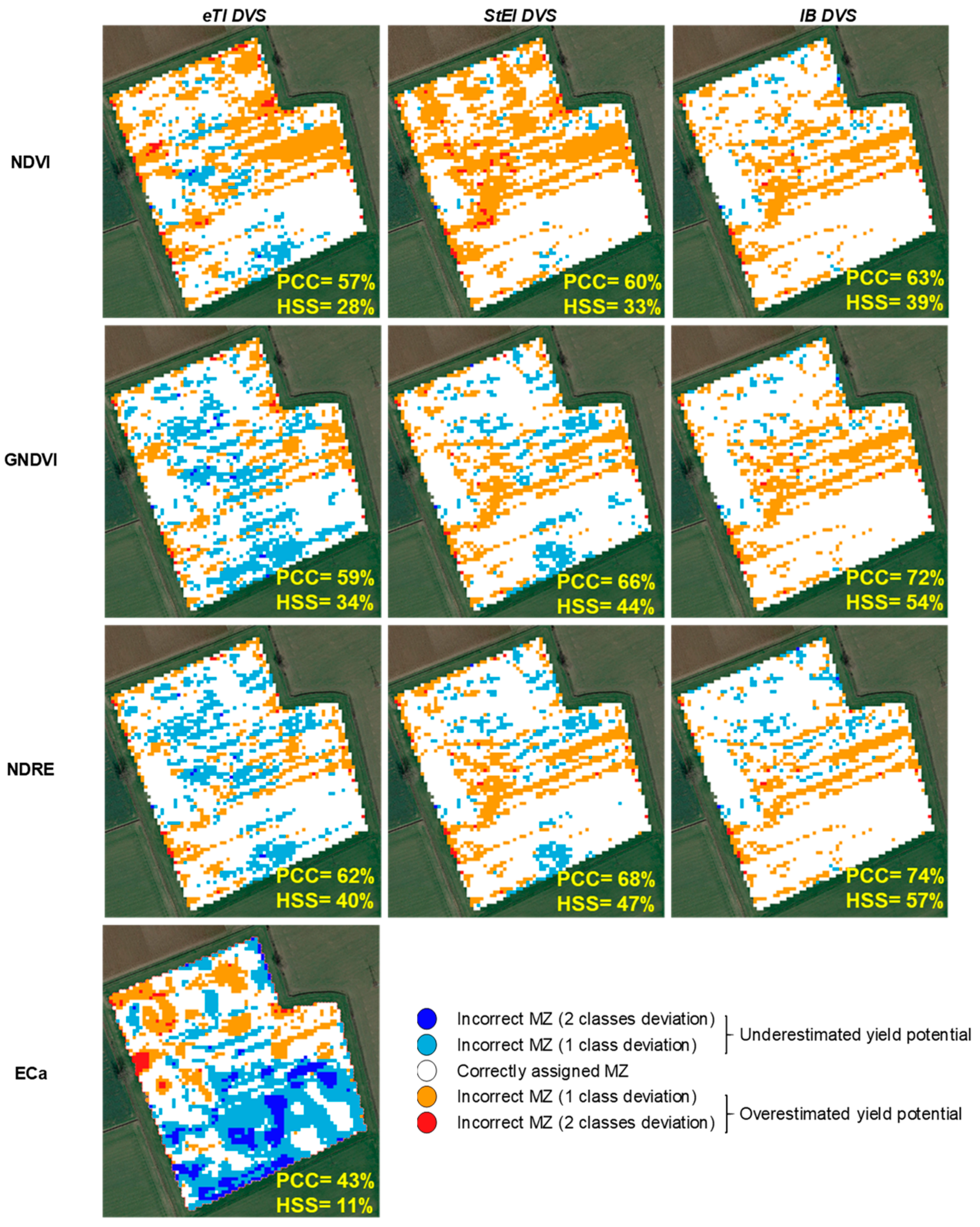
3.3. Site-Specific Accuracy of MZs Mapping

A graphical representation of the accuracy of MZs mapping is presented in Figure 5, and the evaluation metrics are reported in

Table 2. Critical success index (CSI), BIAS, false alarm ratio (FAR), hit rate (H), probability of false detection (F), and the proportion of correct classification (PCC) were calculated separately for soil and vegetation indices, for MZs and development stage (before planting; early tillering, eTl; stem elongation, StEl; late booting, lB).

INDEX	MZ	STAGE	CSI	BIAS	FAR	H	F	PCC
ECA	1	Before Planting	0.27	1.94	0.68	0.62	0.21	0.77
	2		0.34	1.11	0.52	0.53	0.47	0.53
	3		0.19	0.57	0.56	0.25	0.22	0.56
NDVI	1	eTl	0.28	0.54	0.38	0.33	0.03	0.88
		StEl	0.37	0.47	0.16	0.40	0.01	0.91
		lB	0.49	0.59	0.11	0.53	0.01	0.93
	2	eTl	0.33	0.76	0.43	0.43	0.27	0.60
		StEl	0.31	0.61	0.38	0.38	0.19	0.62
		lB	0.31	0.51	0.29	0.36	0.12	0.65
	3	eTl	0.49	1.42	0.44	0.80	0.43	0.66
		StEl	0.53	1.60	0.44	0.90	0.49	0.67
		lB	0.56	1.68	0.43	0.96	0.50	0.69
GNDVI	1	eTl	0.36	1.04	0.48	0.54	0.08	0.87
		StEl	0.50	0.81	0.25	0.60	0.03	0.92
		lB	0.56	0.77	0.17	0.64	0.02	0.93
	2	eTl	0.39	0.92	0.42	0.54	0.32	0.62
		StEl	0.43	0.81	0.33	0.54	0.22	0.67
		lB	0.48	0.72	0.22	0.56	0.13	0.73
	3	eTl	0.48	1.07	0.37	0.68	0.27	0.70
		StEl	0.56	1.27	0.36	0.81	0.32	0.74
		lB	0.63	1.38	0.33	0.92	0.32	0.78
NDRE	1	eTl	0.41	1.31	0.49	0.67	0.10	0.87
		StEl	0.52	0.91	0.28	0.65	0.04	0.92
		lB	0.57	0.93	0.25	0.70	0.04	0.93
	2	eTl	0.43	1.00	0.40	0.60	0.32	0.64
		StEl	0.46	0.87	0.32	0.59	0.23	0.69
		lB	0.52	0.78	0.22	0.61	0.14	0.75
	3	eTl	0.50	0.90	0.29	0.64	0.18	0.74
		StEl	0.56	1.18	0.33	0.78	0.27	0.75
		lB	0.65	1.26	0.30	0.89	0.26	0.80

Statistics in bold font are discussed in the main text.

. Vegetation indices-based maps showed the highest agreement with the Y-MZs map (Figure 5), particularly for the indices based on the G and RE bands (GNDVI and NDRE, respectively), which obtained the highest PCC and HSS scores (Figure 5).

At eTl, GNDVI- and NDRE-MZs maps misclassified grain yield areas in 11% and 19% of the total number of pixels, respectively. On the contrary, the NDVI-MZs map led to a constant yield overestimation throughout the growing season, with 32% (eTl) and 35% (StEl, lB) of pixels leading to 1 or 2 classes mismatch with respect to the Y-MZs map, mostly localized in Y-MZ2. All the vegetation indices obtained better performances at increasing development stages (PCC = 63%, 72%, and 74%; HSS = 39%, 54%, and 57% for NDVI, GNDVI, and NDRE, respectively). Nonetheless, the overestimation of high yield areas increased along with wheat development stages. These errors were concentrated in the transition areas among MZs. Soil-MZs map was characterized by the lowest PCC (43%) and HSS (11%) and by a large number of pixels corresponding to yield underestimation (41%), associated to 1 class (9%) or 2 classes (32%) misclassification. The highest misclassification levels belonged to areas of the field with the highest yield.

The soil-MZs map was characterized by higher accuracy in identifying Y-MZ1 than Y-MZ2 and Y-MZ3 (H value = 0.62), even with overestimation (BIAS = 1.94) in 60% of the pixels (Table 2). The three vegetation indices NDVI, GNDVI, and NDRE led to similar performances in reproducing the Y-MZs map, with higher accuracy (CSI and PCC), reliability (FAR), and discrimination ability (H and F) at increasing development stages (Table 2). At the lB stage, the percentage of correct MZ attribution was high for all indices (PCC > 0.65, CSI > 0.48), whereas NDVI-MZs map failed to identify Y-MZ2 (CSI=0.31) at the StEl stage. Coherently, FAR values decreased during the growing season, indicating lower errors towards crop maturity. The accuracy of the soil and vegetation maps was high in Y-MZ1 (i.e., lowest yield) even at early crop stages (Figure 5, Table 2). The NDVI had lower performances than the other indices, especially considering FAR (0.38 vs. 0.48 and 0.49 for GNDVI and NDRE, respectively) and F (0.03 vs. 0.08 and 0.10 for GNDVI and NDRE, respectively), except at the eTL stage. Moreover, NDVI had the highest BIAS, relative to the MZ3 at late development stages (1.68), probably due to a saturation effect. The NDRE had slightly better performances than GNDVI in MZs definition, with higher discrimination ability. The Y-MZ2 (medium yield) had the highest misclassification rate across soil and vegetation indices.

3.4. Agronomic Evaluation

The areas of the field dedicated to the experimental plots were representative of the identified Y-MZs. The field trial showed that the response of AGB and N uptake to N fertilization, when averaged across the three zones, was positive and significant (p < 0.05) at all development stages (Figure 6 and Figure S5; Tables S3 and S4).

Starting from StEl, AGB and N uptake averaged across N levels were significantly lower in Y-MZ1 than in the other zones (p < 0.05). Finally, from booting onwards, the interaction between N level and management zone was significant (p < 0.05). The response of both dependent variables (AGB and N uptake) to N fertilizer was more flat in Y-MZ1 compared to the other zones. Differences between Y-MZ2 and Y-MZ3 emerged only at harvest, when N uptake in Y-MZ3 was significantly higher (p < 0.05). Therefore, average AGB at harvest in Y-MZ1 was about 70% less than in the other zones (5 vs. 16 t DM ha⁻¹, respectively), while average N uptake was 73 kg N ha⁻¹ in Y-MZ1, 166 kg N ha⁻¹ in Y-MZ2, and 206 kg N ha⁻¹ in Y-MZ3. The plots receiving the same N rate of the whole field (N2; 144 kg N ha⁻¹) led to the following average yields: 2.2, 7.8, and 8.9 t ha⁻¹ in Y-MZ1, Y-MZ2, and Y-MZ3, respectively. The apparent recovery of applied N averaged 29% in Y-MZ1 and 68% in Y-MZ2 and Y-MZ3.

4. Discussion

4.1. Multivariate Analysis

The results showed that Y-MZ1 was the most recognizable area according to any source of information. The clustering carried out on the principal components confirmed that the largest contributors were the lowest ECa values and high reflectance values in the red region of the spectrum, irrespective of the monitoring stage. On the other hand, the relative size of Y-MZ2 and Y-MZ3 differed among development stages. Nonetheless, cluster analysis allowed discovering that NIR and red-edge reflectance values played a major contribution to the definition of Y-MZ2 and Y-MZ3 (Table S2). Our results confirmed the robustness of the red-edge index (NDRE) in the identification of crop status and consequently of MZs, in agreement with previous studies [29,30]. On the contrary, ECa played a minor role in the identification of Y-MZ2 and Y-MZ3 confirming that soil properties were not the only drivers of within-field variability. The crop spectral properties confirmed to be more informative for MZs identification at late wheat development [31,32], especially considering Y-MZ2 and Y-MZ3, even if they were statistically different for N uptake only at harvest. Spectral data acquired during the season allowed differentiating zones with less pronounced agronomic differences, that otherwise would have been uniformly managed.

4.2. Soil-Based MZs Map

The soil-MZs map obtained the highest portion of correct classification of Y-MZ1 (PCC= 0.77), indicating distinct soil properties with respect to the other field zones. The soil texture in Y-MZ1 (lowest yield) was sandy loam (sand = 77%, clay = 11%), whereas in Y-MZ2 and Y-MZ3 was loam (sand = 46%, clay = 17%) and sandy loam (sand = 55%, clay = 14%), respectively. In addition, Y-MZ1 had a lower organic matter content (1.0%) compared to 1.4% and 1.7% measured in Y-MZ2 and Y-MZ3, respectively. The apparent recovery of N in Y-MZ1 was very low (29%), suggesting high N losses or N accumulation in soil, whereas in Y-MZ2 and Y-MZ3, it was in line with previous experiments conducted under similar pedoclimatic conditions [33]. The Y-MZ1 was characterized by limited increases in AGB and N uptake in response to N fertilization (<75 kg N ha⁻¹). Therefore, the main yield-limiting factors in Y-MZ1 (Figure 6) were probably related to the low soil N supply to the crop, the high risk of nitrate leaching due to a coarse texture, and the low soil water content, in turn leading to water stress and reduced crop N availability. The low N availability, likely due to low soil N supply and late winter leaching (Figure S2), could have affected crop growth in Y-MZ1, in addition to water stress during April (stem elongation and booting), when precipitations were scarce (Figure S2).

This study confirmed that the sole consideration of soil properties in MZs mapping is not sufficient [32] and it could rather have led to the erroneous definition of Y-MZ2 and Y-MZ3. The difference in yield between Y-MZ2 and Y-MZ3 was probably caused by the interaction of soil properties with agricultural management factors, not accounted by soil survey. This is proved by the fact that soil-MZs classified correctly only 25% of Y-MZ3 with marked yield underestimation (BIAS = 0.57). Moreover, the soil-MZs map showed large spatial variability within the field that was not reflected by Y-MZs (Figure 4). This suggested that the effect of soil properties on grain yield was partially masked by management and meteorological factors, in agreement with other studies [8,34].

4.3. Vegetation-Based MZs Map

According to literature, the effects of local agronomic management and weather variability can be captured by vegetation indices [32], which in our study were more reliable than soil data for in-season MZs definition. The accuracy of VI-MZs maps increased along with wheat development, confirming that in-season monitoring allowed capturing the dynamics of crop growth, up to yield formation [9]. However, despite the site-specific accuracy of the VI-MZs maps increased, also the yield overestimation increased (Figure 5). This indicates a saturation effect common to all the vegetation indices, which occurs when vegetation is still growing while the indices had already reached their maximum value [35]. This situation emerged since StEl in large areas of the field (35%, 20%, and 23% of the total field area for NDVI, GNDVI, and NDRE, respectively), which were erroneously transitioned from Y-MZ2 to Y-MZ3 because of high values of the vegetation indices. According to literature, our results confirmed that the red-based vegetation index (NDVI) was more affected by saturation than GNDVI and NDRE [36].

The cumulative vegetation indices probably suffered by saturation effect at earlier crop monitoring and did not lead to better results than the simple indices, according to Wang et al. (2014) [37] but in contrast to other studies [25,38]. It could be explained by the less sensitivity to crop growth dynamics due to a carry-over effect of the information of previous surveys [25]. One of the main evidence of our study is that AGB values and the crop N response were statistically different among Y-MZs from late booting, whereas vegetation indices were able to correctly reproduce Y-MZs since early wheat development. As a consequence, a minimum dataset for reliable MZs map definition can be defined as one vegetation index (RE-based, G-based, and even R-based at very early crop stages) collected between early tillering and stem elongation, which are also two key stages for wheat N side-dress fertilization.

5. Conclusions

Italian farmers are experiencing a transition from standard to precision agriculture and need simple and low-input procedures to support the shift of paradigm. This study evaluated the reliability of alternative data sources acquired by high-resolution soil and crop sensors when no past knowledge of the within-field variability is available. We demonstrated that soil-based maps were not able to reproduce the actual yield levels, whereas crop monitoring led to high accuracy, reliability, and discrimination ability in MZs mapping. The optimal source of information and timing of field survey were identified to allow a low-input and effective yield mapping of winter cereals: RE-based indices with a NIR component (coming from aerial or satellite surveys) collected from early tillering to stem elongation, which can be processed with simple statistical methods and open-source software could identify Y-MZs. Finally, despite the stability of MZs could be improved during the years with new yield maps, low-input, in-season crop monitoring demonstrated to be able to effectively support farmer management since early crop stages identifying MZs that could be effectively managed with different N rates. In fact, from an agronomical point of view, the identification of Y-MZ1, using the proposed procedure integrated with the results of the plot trial for the evaluation of N rates, suggested to reduce N fertilization in Y-MZ1 by about 50% with clear economic and environmental benefits. However, identified Y-MZ2 and Y-MZ3 that produced close but statistically different yields (7 and 9 t DM ha⁻¹, respectively) would require a long-term evaluation to clearly identify the possibility of adopting different fertilization strategies.

References

1. Ramankutty, N.; Mehrabi, Z.; Waha, K.; Jarvis, L.; Kremen, C.; Herrero, M.; Rieseberg, L.H. Trends in global agricultural land use: Implications for environmental health and food security. Annu. Rev. Plant Biol. 2018, 69, 789–815. [Google Scholar] [CrossRef] [PubMed] [Green Version]
2. Taylor, J.; Whelan, B. A General Introduction to Precision Agriculture; Australian Center for Precision Agriculture. 2005. Available online: http://www.agriprecisione.it/wp-content/uploads/2010/11/general_introduction_to_precision_agriculture.pdf (accessed on 29 July 2020).
3. Lemaire, G.; Jeuffroy, M.-H.; Gastal, F. Diagnosis tool for plant and crop N status in vegetative stage: Theory and practices for crop N management. Eur. J. Agron. 2008, 28, 614–624. [Google Scholar] [CrossRef]
4. Grisso, R.D.; Alley, M.M.; Thomason, W.E.; Holshouser, D.L.; Roberson, G.T. Precision Farming Tools: Variable-Rate Application. 2011. Available online: https://vtechworks.lib.vt.edu/bitstream/handle/10919/47448/442-505_PDF.pdf (accessed on 29 July 2020).
5. Holland, K.H.; Schepers, J.S. Derivation of a variable rate nitrogen application model for in-season fertilization of corn. Agron. J. 2010, 102, 1415–1424. [Google Scholar] [CrossRef]
6. Solie, J.B.; Monroe, A.D.; Raun, W.R.; Stone, M.L. Generalized algorithm for variable-rate nitrogen application in cereal grains. Agron. J. 2012, 104, 378–387. [Google Scholar] [CrossRef] [Green Version]
7. Dammer, K.-H.; Wartenberg, G. Sensor-based weed detection and application of variable herbicide rates in real time. Crop. Prot. 2007, 26, 270–277. [Google Scholar] [CrossRef]
8. Nawar, S.; Corstanje, R.; Halcro, G.; Mulla, D.; Mouazen, A.M. Delineation of soil management zones for variable-rate fertilization. Adv. Agron. 2017, 143, 175–245. [Google Scholar] [CrossRef]
9. Long, D.S.; Carlson, G.R.; De Gloria, S.D. Quality of field management maps. Site Specif. Manag. Agric. Syst. 1995, 251–271. [Google Scholar] [CrossRef]
10. Mulla, D.J. Using geostatistics and GIS to manage spatial patterns in soil fertility. In Automated Agriculture for the 21st Century; Kranzler, G., Ed.; ASAE: Niles, MI, USA, 1991; pp. 336–345. [Google Scholar]
11. Stewart, C.M.; McBratney, A.B.; Skerritt, J.H. Site-specific durum wheat quality and its relationship to soil properties in a single field in northern New South Wales. Precis. Agric. 2002, 3, 155–168. [Google Scholar] [CrossRef]
12. Shaner, D.L.; Khosla, R.; Brodahl, M.K.; Buchleiter, G.W.; Farahani, H.J. How well does zone sampling based on soil electrical conductivity maps represent soil variability? Agron. J. 2008, 100, 1472–1480. [Google Scholar] [CrossRef] [Green Version]
13. Schenatto, K.; Souza, E.G.; Bazzi, C.L.; Bier, V.A.; Betzek, N.M.; Gavioli, A. Data interpolation in the definition of management zones. Acta Sci. Technol. 2016, 38, 31–40. [Google Scholar] [CrossRef] [Green Version]
14. Casa, R.; Pelosi, F.; Pascucci, S.; Fontana, F.; Castaldi, F.; Pignatti, S.; Pepe, M. Early stage variable rate nitrogen fertilization of silage maize driven by multi-temporal clustering of archive satellite data. Adv. Anim. Biosci. 2017, 8, 288–292. [Google Scholar] [CrossRef]
15. Ortuani, B.; Sona, G.; Ronchetti, G.; Mayer, A.; Facchi, A. Integrating geophysical and multispectral data to delineate homogeneous management zones within a vineyard in Northern Italy. Sensors 2019, 19, 3974. [Google Scholar] [CrossRef] [PubMed] [Green Version]
16. Rampant, P.; Abuzar, M. Geophysical tools and digital elevation models: Tools for understanding crop yield and soil variability. Proceedings of SuperSoil 2004: 3rd Australian New Zealand Soils Conference, Sydney, Australia, 5–9 December 2004; University of Sydney: Sydney, Australia, 2004; pp. 1–9. [Google Scholar]
17. Pascucci, S.; Carfora, M.; Palombo, A.; Pignatti, S.; Casa, R.; Pepe, M.; Castaldi, F. A comparison between standard and functional clustering methodologies: Application to agricultural fields for yield pattern assessment. Remote Sens. 2018, 10, 585. [Google Scholar] [CrossRef] [Green Version]
18. De Benedetto, D.; Castrignano, A.; Diacono, M.; Rinaldi, M.; Ruggieri, S.; Tamborrino, R. Field partition by proximal and remote sensing data fusion. Biosyst. Eng. 2013, 114, 372–383. [Google Scholar] [CrossRef]
19. Khosla, R.; Inman, D.; Westfall, D.G.; Reich, R.M.; Frasier, M.; Mzuku, M.; Koch, B.; Hornung, A. A synthesis of multi-disciplinary research in precision agriculture: Site-specific management zones in the semi-arid western Great Plains of the USA. Precis. Agric. 2008, 9, 85–100. [Google Scholar] [CrossRef]
20. Guastaferro, F.; Castrignanò, A.; De Benedetto, D.; Sollitto, D.; Troccoli, A.; Cafarelli, B. A comparison of different algorithms for the delineation of management zones. Precis. Agric. 2010, 11, 600–620. [Google Scholar] [CrossRef]
21. Lancashire, P.D.; Bleiholder, H.; Boom, T.; van den Langelüddeke, P.; Stauss, R.; Weber, E.; Witzenberger, A. A uniform decimal code for growth stages of crops and weeds. Ann. Appl. Biol. 1991, 119, 561–601. [Google Scholar] [CrossRef]
22. Pebesma, E.; Heuvelink, G. Spatio-temporal interpolation using gstat. RFID J. 2016, 8, 204–218. [Google Scholar]
23. Ricotta, C.; Avena, G.; De Palma, A. Mapping and monitoring net primary productivity with AVHRR NDVI time-series: Statistical equivalence of cumulative vegetation indices. ISPRS J. Photogramm. Remote Sens. 1999, 54, 325–331. [Google Scholar] [CrossRef]
24. Lê, S.; Josse, J.; Husson, F. FactoMineR: An R package for multivariate analysis. J. Stat. Softw. 2008, 25, 1–18. [Google Scholar] [CrossRef] [Green Version]
25. R Development Core Team. R: A Language and Environment for Statistical Computing; R Foundation for Statistical Computing: Vienna, Austria, 2008; ISBN 3-900051-07-0. Available online: http://www.r-project.org (accessed on 29 July 2020).
26. Fridgen, J.J.; Kitchen, N.R.; Sudduth, K.A.; Drummond, S.T.; Wiebold, W.J.; Fraisse, C.W. Management zone analyst (MZA). Agron. J. 2004, 96, 100–108. [Google Scholar] [CrossRef]
27. Martínez-Casasnovas, J.A.; Arnó, J. Use of farmer knowledge in the delineation of potential management zones in precision agriculture: A case study in maize (Zea mays L.). Agriculture 2018, 8, 84. [Google Scholar]
28. Wilks, D.S. Statistical Methods in the Atmospheric Sciences; Elsevier: Amsterdam, The Netherlands; Academic Press: Amsterdam, The Netherlands, 2011. [Google Scholar]
29. Tavakoli, H.; Mohtasebi, S.S.; Alimardani, R.; Gebbers, R. Evaluation of different sensing approaches concerning to non-destructive estimation of leaf area index (LAI) for winter wheat. Int. J. Smart Sens. Intell. Syst. 2014, 7, 337–359. [Google Scholar]
30. Corti, M.; Cavalli, D.; Cabassi, G.; Gallina, P.M.; Bechini, L. Does remote and proximal optical sensing successfully estimate maize variables? A review. Eur. J. Agron. 2018, 99, 37–50. [Google Scholar] [CrossRef]
31. Marino, S.; Alvino, A. Detection of homogeneous wheat areas using multi-temporal UAS images and ground truth data analyzed by cluster analysis. Eur. J. Remote Sens. 2018, 51, 266–275. [Google Scholar] [CrossRef] [Green Version]
32. Maestrini, B.; Basso, B. Predicting spatial patterns of within-field crop yield variability. Field Crop. Res. 2018, 219, 106–112. [Google Scholar] [CrossRef]
33. Cavalli, D.; Cabassi, G.; Borrelli, L.; Geromel, G.; Bechini, L.; Degano, L.; Marino Gallina, P. Nitrogen fertilizer replacement value of undigested liquid cattle manure and digestates. Eur. J. Agron. 2016, 73, 34–41. [Google Scholar] [CrossRef]
34. Schepers, A.R.; Shanahan, J.F.; Liebig, M.A.; Schepers, J.S.; Johnson, S.H.; Luchiari, A. Appropriateness of management zones for characterizing spatial variability of soil properties and irrigated corn yields across years. Agron. J. 2004, 96, 195–203. [Google Scholar] [CrossRef] [Green Version]
35. Xia, T.; Miao, Y.; Wu, D.; Shao, H.; Khosla, R.; Mi, G. Active optical sensing of spring maize for in-season diagnosis of nitrogen status based on nitrogen nutrition index. Remote Sens. 2016, 8, 605. [Google Scholar] [CrossRef] [Green Version]
36. Scotford, I.M.; Miller, P.C.H. Applications of spectral reflectance techniques in Northern European cereal production: A review. Biosyst. Eng. 2005, 90, 235–250. [Google Scholar] [CrossRef]
37. Wang, L.; Tian, Y.; Yao, X.; Zhu, Y.; Cao, W. Predicting grain yield and protein content in wheat by fusing multi-sensor and multi-temporal remote-sensing images. Field Crop. Res. 2014, 164, 178–188. [Google Scholar] [CrossRef]
38. Zhou, X.; Zheng, H.B.; Xu, X.Q.; He, J.Y.; Ge, X.K.; Yao, X.; Cheng, T.; Zhu, Y.; Cao, W.X.; Tian, Y.C. Predicting grain yield in rice using multi-temporal vegetation indices from UAV-based multispectral and digital imagery. ISPRS J. Photogramm. Remote Sens. 2017, 130, 246–255. [Google Scholar] [CrossRef]
Figure 1. Schematic representation of the activities carried out in the study. * EMI = electromagnetic induction; UAV = unmanned aerial vehicle; ECa: apparent electrical conductivity; MZ: management zone.
Agronomy 10 01124 g001
Figure 2. Example of 3-classes contingency matrix and its reduction to one table for each class (dichotomous tables).
Agronomy 10 01124 g002
Figure 3. Results of principal component analysis (PCA). PCA score plots of individuals (pixels) showing the pixels in the first two principal components space marked according to (a) the yield-based management zones, and (b) the development stages at the time of crop monitoring (DVS: 1, 2, and 3 corresponded to eTl, StEl, and lB). (c) PCA plot of the original variables projected into the first two principal components space. (d) PC score-plot showing the three extracted clusters.
Agronomy 10 01124 g003
Figure 4. Management zone (MZ) maps resulting from yield data; NDVI measured at early tillering stage (eTl), stem elongation stage (StEl), late booting stage (lB); cumulative NDVI (cumNDVI); ECa. For each map and MZ, the mean value and the coefficient of variation (CV) of the predictor is reported, as well as the average yield and the covered area.
Agronomy 10 01124 g004
Figure 5. Graphical representation of the differences between the reference yield-based MZs map and the MZs maps based on vegetation indices acquired at three different development stages (NDVI, GNDVI, and NDRE), and ECa. For each map, the proportion of correct classification (PCC) MZs attribution, and the Heidke skill score (HSS) are reported.
Agronomy 10 01124 g005
Figure 6. Mean N uptake values from the field trial presented separately by the time of monitoring survey, by nitrogen level (N0 = 0 kg N ha−1; N72 = 72 kg N ha−1; N144 =144 kg N ha−1) and by field zone (1, 2, and 3 representatives of low MZ1, medium MZ2, and high MZ3 grain yield, respectively). Error bars represent the standard error of the mean.
Agronomy 10 01124 g006