Article

Investigating Sentinel 2 Multispectral Imagery Efficiency in Describing Spectral Response of Vineyards Covered with Plastic Sheets

by
Enrico Borgogno-Mondino
1,
Laura de Palma
2,* and
Vittorino Novello
1
1
Department of Agricultural, Forestry and Food Sciences, University of Turin, I-10095 Turin, Italy
2
Department of Sciences of Agriculture, Food, Natural Resources and Engineering, University of Foggia, 25-71121 Foggia, Italy
*
Author to whom correspondence should be addressed.
Agronomy 2020, 10(12), 1909; https://doi.org/10.3390/agronomy10121909
Submission received: 4 November 2020 / Revised: 28 November 2020 / Accepted: 30 November 2020 / Published: 2 December 2020

Abstract

:
The protection of vineyards with overhead plastic covers is a technique largely applied in table grape growing. As with other crops, remote sensing of vegetation spectral reflectance is a useful tool for improving management even for table grape viticulture. The remote sensing of the spectral signals emitted by vegetation of covered vineyards is currently an open field of investigation, given the intrinsic nature of plastic sheets that can have a strong impact on the reflection from the underlying vegetation. Baring these premises in mind, the aim of the present work was to run preliminary tests on table grape vineyards covered with polyethylene sheets, using Copernicus Sentinel 2 (Level 2A product) free optical data, and compare their spectral response with that of similar uncovered vineyards to assess if a reliable spectral signal is detectable through the plastic cover. Vine phenology, air temperature and shoot growth, were monitored during the 2016 growing cycle. Twenty-four Copernicus Sentinel 2 (S2, Level 2A product) images were used to investigate if, in spite of plastic sheets, vine phenology can be similarly described with and without plastic covers. For this purpose, time series of S2 at-the-ground reflectance calibrated bands and correspondent normalized difference vegetation index (NDVI), modified soil-adjusted vegetation index, version two (MSAVI2) and normalized difference water index (NDWI) spectral indices were obtained and analyzed, comparing the responses of two covered vineyards with different plastic sheets in respect of two uncovered ones. Results demonstrated that no significant limitation (for both bands and spectral indices) was introduced by plastic sheets while monitoring spectral behavior of covered vineyards.

1. Introduction

Grapes are one of the most commonly consumed fruits worldwide (77.8 million tons were harvested in 2018), with grapevine cultivation being widely spread across the five continents (7.4 million hectares in 2018). Additionally, table grape production has doubled in the last twenty years to currently represent 35% of total world grape production [1].
The protection of vineyards with plastic covers is a widespread technique in several grapevine growing regions, especially in those where table grapes are produced: it is aimed at preserving both vegetation and grapes from external agents and/or conditioning the microclimate to extend the harvest period by advancing or delaying grape harvest [2]. Generally speaking, crop covers may exert positive effects such as enforcing the production system [3], increasing the rate of plant growth and development [4] and inducing a significant improvement in fruit quality [5,6]. Plastic sheets are known to interact with the incoming sun radiation changing its intensity and quality as it passes through them. Changes in solar radiation directly affect the physiology and morphology of plants [7,8] as a function of cover spectroradiometric properties such as light-dispersive capacity and wavelength selectivity [4,9]. Sheets (or nets) for crop protection against weather, diseases, virus-vector insects and birds are used as stand-alone coverings or jointly with crop support trellises. Despite the advantages that covers can provide, their use also has disadvantages. From a landscape point of view, they certainly degrade the aesthetical features of the rural landscape, introducing large-scale artefacts that alter the original view of countryside. Secondly, large quantities of plastic sheets have to be frequently removed and substituted, impacting the plastic waste cycle; finally, they represent a potential source of environmental pollution that could dramatically affect the local agro-ecosystem in case of abandonment or uncontrolled combustion [10].
Natural variability of plant and field conditions, as well as erratic application of cultural practices, influence quantity and quality of crop production. Mapping of cultivated plots helps crop management by monitoring plant growth [11], enhancing the precision of input deliveries, and possibly forecasting the yield quality and quantity trends.
Among the currently available environmental analysis tools, remote sensing techniques can be applied to detect and map plastic-covered vineyards with the aim of supporting/addressing appropriate policies for a better planning and managing of viticultural practices. Within this context, an important issue is to point out if—and how—plastic covering can affect remote sensing-based analysis. Some studies report preliminary results suggesting that plastic sheets are not a problem for satellite or airborne recognition [12,13]. Nonetheless, the remote sensing of spectral signals emitted by vegetation covered with plastic materials is currently an open field of investigation, given the intrinsic nature of plastic covers, especially as concerns their close-to-specular reflecting behavior, that can have a strong impact on the detection of reflectance signals. They interact with the process of radiative transfer from vegetation to surrounding environment, introducing further and unknown factors possibly also related to the lighting conditions. Therefore, plastic sheets are expected to change the transmission and absorption signals and generate reflection artifacts. In this context, when trying to monitor/study crop behavior by remote sensing, a multi-temporal approach must be used [14]. Medium resolution satellite imagery has already proved to be effective at the vineyard level to describe shoot vigor, vine and soil water status, and their seasonality. This is an important issue to focus on since, this type of images being often free, the entire process could be economic enough to be consistent with costs and incomes of ordinary farming company [15,16].
With these premises, the aim of the present work was to run preliminary tests on table grape vineyard plots covered with polyethylene sheets using Copernicus Sentinel 2 (S2, Level 2A product) free optical data (European Space Agency, European Union), and compare their spectral response with that of similar uncovered vineyards in order to test whether, through overhead plastic sheets that protect vineyard canopy, reliable spectral signals can be detected.

2. Materials and Methods

2.1. Study Area and Test Vineyards

Two adjacent 1 hectare table grape vineyards (5 year old) realized with same plant materials (cv. Victoria/1103 P) in South Italy (Apulia Region, BT Province, Laporta farm, Figure 1) were used as references to represent covered vineyards. They were covered from 10 March to the end of October 2016, using two types of plastic sheets characterized by different spectroradiometric properties [17]. Coverlys agrotextile (Beaulieu Technical Textiles, Comines-Warneton, Belgium) and Serrosol film (Serroplast, Rutigliano, BA, Italy) were used to cover the two vineyards named as vineyard C and vineyard S, respectively. Both sheets were made of polyethylene with some additives, were transparent to solar radiation and had a thickness of 200 μm. Two uncovered vineyards (hereinafter called V1, V2) of about 1 ha each, having the same age, were selected in the nearby area at a distance of 1.67 km apart in a straight line, and were assumed to represent ordinary local uncovered vineyards. All vineyards were trained to tendone trellis with same vine distance (2.4 × 2.4 m). The vines received viticultural practices normally applied in the growing area; moreover, in the covered vineyards, the cane and shoot number per vine was uniformed by winter and summer pruning.

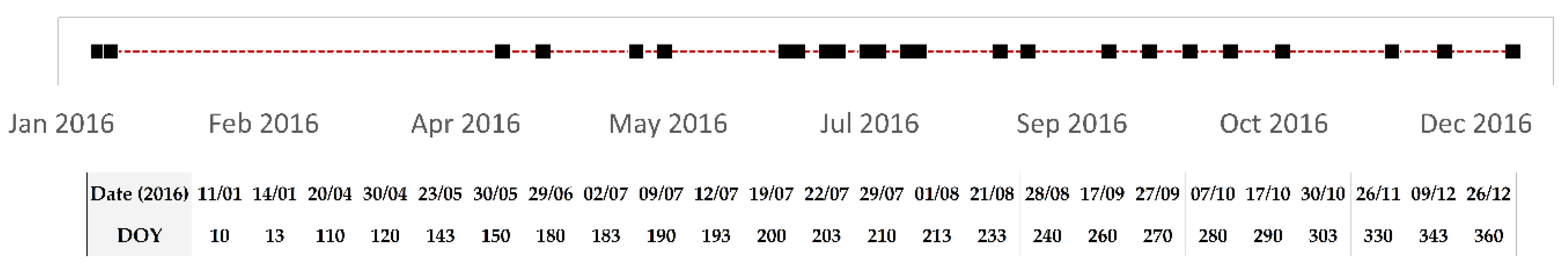
2.2. Available Satellite Data

Twenty-four Copernicus Sentinel-2 Level 1C images were obtained from Google Earth Engine [18]. L1C product consists of a 100 km2 tile orthoprojected in the WGS84 UTM 33N system and calibrated in TOA (top-of-atmosphere) reflectance. Main features of Sentinel 2 (S2) data are reported in Table 1. Dates of acquisition are reported in the table associated to Figure 2. Only images with no clouds over the vineyards of interest where considered for the 2016 growing season, namely 24 out of the 36 images available in the reference period.
S2 L1C data were preventively converted to BOA (bottom-of-atmosphere) format by the Sen2Cor procedure available in the free SNAP software (ESA, European Union).

2.3. Available Ground Data

Air temperature was continuously recorded, at 2 m height above ground level, within C and S covered vineyards and in open air. ECH2O sensors equipped with data loggers (Decagon Devices Inc., Pullman, WA, USA) were used for this purpose. Air temperature data were used to compute the correspondent growing degree days (GDD) in the period 1 April 2016–30 July 2016 (grape harvest) according to Winkler Equation (1) [19]:
G D D ( t ) =   i = 0 t ( T m ( i ) 10 ° ) i    
where t is the number of days from the starting date of GDD calculation (1 April), Tm is the local air daily mean temperature (°C) and 10 °C is the reference base temperature for grapevine.
Weekly, vine phenology was monitored and reported to the BBCH (Biologische Bundesantalt, Bundessortenamt and Chemische Industrie) scale according to Lorenz and collaborators [20], and length of primary shoot of covered vines was measured, from bud break to fruit set, at all nodes of two canes sampled on 10 vines per plot.

2.4. Testing Spectral Differences: Bands and Indices

For this study, only bands 2–8, 8a, 11 and 12 were considered, being the most suitable and used ones for horticultural purposes from both spectral and geometrical point of view [21]. Bands 1, 9 and 10, having a coarser geometric resolution (60 m) were not considered since mainly designed for atmosphere characterization and being geometrically not consistent with vineyard sizes.
Three spectral vegetation indices were initially selected: the normalized difference vegetation index (NDVI, Equation (2)), the modified soil-adjusted vegetation index, version 2 (MSAVI2, Equation (3)) and the normalized difference water index (NDWI, Equation (4)):
NDVI = ( ρ b 8 ρ b 4 ) ( ρ b 8 + ρ b 4 )
MSAVI 2 = [ 2 × ρ b 8 + 1 ( 2 × ρ b 8 + 1 ) 2 8 × ( ρ b 8 ρ b 4 ) ] 2
NDWI = ( ρ b 8 ρ b 11 ) ( ρ b 8 + ρ b 11 )
where ρ b 8 , ρ b 4 and ρ b 12 are the at-the-ground reflectance of band 8, band 4 and band 12, respectively.
NDVI is widely adopted to describe vegetation phenology along the growing season, being correlated with biomass development and plant health status [22]. MSAVI2, is an alternative vegetation index, with respect to NDVI, that is generally considered more suitable when the monitored vegetation alternates with a not-vegetated background [23]; this is exactly the situation that occurs in table grape vineyards from bud-break until shoots overlay the trellis roof. Both the indices range between −1 and +1, moving towards higher values when biomass content of pixel increases. MSAVI2 is said to minimize spectral effects of soil when the monitored vegetation is discontinuous (vineyards, orchards, starting phases of crops). If monitored at pixel (or plot) level along time, NDVI and MSAVI2 are good predictors of phenology. Unexpected anomalies along the profile could suggest problems related to the ordinary development of vines. Additionally, spatial distribution of NDVI/MSAVI2 at the same date permits to compare the status of different vineyards (or parts of the same vineyard) allowing a better focused management strategy. NDWI is used to describe vegetation water content. Similarly to NDVI and MSAVI2, it ranges between −1 and +1. The higher the value, the higher the water content. If interpreted along a time series at the pixel (or plot) level to detect water content changes, it must be preventively assured that no significant change in biomass occurs within the explored period (i.e., NDVI or MSAVI2 do not change significantly) [24]. Differently, its spatial distribution at a certain date makes it possible to compare the water content status of different vineyards (or parts of the same vineyard).
Complementarity of NDVI and MSAVI2 was preventively analyzed to explore if and how they could somehow describe different the properties of the vegetative behavior of vines. Comparison was achieved by scatterplot construction, and concerned both mean and standard deviation values as computed at plot level (4 vineyards) along the entire observation period (24 images). Since a strong correlation was found, a 2nd order polynomial function was selected to fit existing relationship.
The second step concerned the extraction and comparison of the spatially averaged temporal profiles of bands and NDVI/NDWI from each of the four vineyards. Spatial distribution of reflectance within each vineyard was also investigated. The coefficient of variation (CV) (Equation (5)) was accordingly computed for each plot and for each date:
CV j ( t ) = σ j i ( t ) μ j i ( t ) × 100
where μ j i ( t ) and σ j i (t) are the mean and standard deviation values of the i-th band/spectral index for the j-th vineyard; t is the date of acquisition.
To verify if inter-vineyard spectral differences were significant, the Wilcoxon rank-sum approach was adopted. It tests the hypothesis that two sample populations X and Y have the same median of distribution against the hypothesis. The result is the nearly-normal test statistic Z and the one-tailed probability of obtaining a value of the absolute value of Z or greater.

2.5. Biophysical Effects of Differences: NDVI Versus GDD

To investigate the persistence of the biophysical meaning of NDVI under plastic films, the well-known relationship between NDVI and GDD [19] was tested for the 4 vineyards. It is worth reminding that such a relationship is well modeled by a second order polynomial, according to Equation (6) [25,26]:
NDVI ( t ) = a × GDD 2 ( t ) + b × GDD ( t ) + c
where a, b and c are the coefficients to be estimated by the ordinary least squares according to satellite (NDVI) and ground (GDD) data. Once the model of Equation (6) was calibrated, the following phenological parameters were obtained:
GDD max = B 2 A
NDVI max = C B 2 4 A
where GDDmax is the GDD value of the day when the maximum NDVI (NDVImax) is reached along the season.
A further relationship was then calibrated and modelled relating GDD to DOY according to Equation (9).
DOY = a × GDD b
where a and b are the coefficients to be estimated by the ordinary least squares.
Only 12 of the available images proved to be useful for model calibration, given the starting and ending dates of the GDD computation from ground data (from 1 April 2016 to 2 August 2016).

3. Results and Discussion

The correlation between NDVI and MSAVI2 was found to be very high both in terms of mean values (R2 > 0.99 at p < 0.001) and standard deviations (R2 = 0.86, p < 0.001). Consequently, in spite of the expected benefits reported in the literature [23], MSAVI2 did not provide any additional information in respect to NDVI (Figure 3). The former was thus not considered for further evaluations.

3.1. Temporal Trends of Vegetation Reflectances/Indices (Mean Values)

With respect to the main goal of this work, concerning the exploration of the contribution of plastic films to spectral information obtainable from covered vineyards, a first analysis was conducted generating, at the vineyard level, time trends of bands and vegetation index (Figure 4 and Figure 6).
The two covered vineyards showed very similar profiles for all the bands and indices. Vineyard C exhibited a slight tendency for a higher reflectance in the visible wavelength range, which is mostly related to the plant pigments. However, this trend was more evident for measurements taken from DOY 240, i.e., when vine shoots were no longer growing and wood maturation occurs (BBCH 90), to DOY 303, i.e., when leaves were discoloring (BBCH 92); therefore, the observed differences could be possibly due to factors other than the evolution of the vine canopy, such as a dissimilar growth of weeds on the soil. NDVI and NDWI showed a tendency for higher values in S vineyard, especially from DOY 143, that corresponded to the beginning of berry set (BBCH 71), i.e., when the growth of the vine shoots normally starts to decline, to DOY 260 (BBCH 90). This trend is corroborated by that of primary shoot growth, which showed a slightly higher rates in vineyard S than in vineyard C (Figure 5). Either primary or secondary shoot length have been proved to be well correlated with total leaf area per shoot as well as with fresh and dry shoot leaf mass [27]; since, in the present study, vine growing conditions and shoot number per vine of covered vineyards had been uniformed, it is reasonable to assume that difference in primary shoot length was indicative of differences in leaf area and leaf mass. Hence, information provided by the two indices seemed more realistic than those provided by single spectral bands. Moreover, NDVI and NDWI profiles indicate a noticeable presence of biomass even at the beginning and at the end of the season, i.e., when vines are still dormant and when they are shedding or have lost their leaves: this spectral response could be possibly related to an invasive grass growth in periods when cultural practices are suspended.
Spectral bands and indices of the two uncovered vineyards also showed quite similar profiles. V1 exhibited a slight tendency for a higher reflectance especially in the visible part of the spectrum (Figure 6). Comparing bands/indices temporal profiles of S and C covered vineyards (Figure 4) with those of V1 and V2 uncovered ones (Figure 6), a major presence of biomass can be noted in V1 and V2 before bud-breaking (at the first two dates of measurements); moreover, at the end of the season, V1 and V2 NDVI profiles showed a wider plateau, resisting until the end of October (DOY 280). Differently, S and C vineyards reduced most of their reflectance at the end of August (DOY 240). No other relevant difference can be observed in the profile shape nor in the reflectance values.
Overall, the similarity of the spectral profiles detected in the two vineyards covered with different types of plastic sheets, the small profile diversity of covered and uncovered vineyards, and the explainability of the observed differences suggest that the plastic covers had a low impact on S2 collected data.
Significance of profile differences was tested for according to the Wilcoxon rank-sum test and Pearson’s R coefficient computation. Results are reported in Table 2. No statistically significant difference (at p < 0.05) was found between temporal profiles of S and C covered vineyards, for all the bands. R values confirmed a significant similarity between temporal profiles of all the bands. Differences between S covered vineyard and V1 and V2 uncovered ones were significant for almost all the bands in both the cases, with the exception of bands 7, 8, 8a in the comparison with V1.
Differences between C covered vineyard and V1 and V2 uncovered ones were significant for visible (b2–b4) and short wavelength infrared (SWIR) (b11, b12) bands. Bands b2 and b11 showed the highest degree of difference, that was marked and significant in the comparisons C vs. V1 and C vs. V2. Bands closer to the near infrared (NIR) region showed the lowest differences (see at C vs. V1 and S vs. V2). However, even most of the significant differences seemed to not be strong enough to move R values out of the correlation area or to considerably affect spectral indices. Indices seemed to absorb most of band differences, proving to be robust analysis tools for investigating vineyard spectral behavior regardless of the presence of plastic covers.

3.2. Temporal Trends of Spatial Variability of Reflectances/Indices within Vineyards

The above discussed results demonstrated that no statistically significant difference could be recognized when monitoring the average spectra behavior of covered and uncovered vineyards; nevertheless, a definitive conclusion about the role of plastic sheets requires that spatial variability of spectral properties within vineyards is also tested. Consequently, with reference to CV (Equation (5)), the temporal profiles along the year were generated for all the vineyards, and statistical significance of differences tested by the Wilcoxon rank-sum test and Pearson’s R coefficient. Trends are reported in Figure 7 and Figure 8; test statistics are reported in Table 3.
Concerning intra-vineyard spatial distribution of reflectance within S and C covered vineyards (Figure 7), the yearly trends showed that: (a) in the visible range, b4 (red) appeared to express the highest intra-vineyard variability for both S and C (up to 30%). The time pattern was slightly different in the two vineyards; (b) a reduced, and almost constant, variability affected NIR/red edge bands (5–10%) with a springer exception probably due to time series filtering problems; (c) SWIR bands (b11 and b12) appeared to be highly varying within the vineyards, with a prevalence of b12. Again, S and C showed similar but not equal time pattern; (d) spectral indices (NDVI and NDWI) similarly showed a high intra-vineyard variability with no significant seasonal behavior if not at the beginning and at the end of the season.
These results could be related to the fact that at the beginning of the season vine canopies are not still developed while in the last part of the season they start to decline. Oppositely, quite stable values were found in the central part of the season, when vine canopies are already expanded and covere the vineyard trellis; in general, S vineyard proved to be more heterogeneous in terms of both CV value and seasonality.
Concerning intra-vineyard spatial distribution of reflectance within V1 and V2 uncovered vineyards (Figure 8), it was found that: (a) in the visible range, b4 (red) appeared to express the highest intra-vineyard variability for both vineyards. Nevertheless, V2 showed the highest variability (up to 40%). The time pattern was slightly different in the two vineyards; (b) a reduced, but not timely constant, variability affected NIR/red edge bands with no springer exception in this case; in this spectral range, b8a showed the highest CV values; (c) SWIR bands (b11 and b12) appeared to be highly varying only in V2. Variability of b12 was confirmed to prevail on that of b11; (d) spectral indices (NDVI and NDWI) showed a high intra-vineyard variability with no significant seasonal behavior.
Concluding, it can be said that common general tendencies were found for both covered and uncovered vineyards. The logic of these results and the similarity of the trends observed between covered and uncovered vineyards lead us to consider that the spectral response, as detected through plastic coverings, was quite reliable.

3.3. GDD vs. NDVI Viticultural Meaning

In order to further investigate if spectral signals from covered vineyards could generate reliable information on vine behavior, the well-known relationship between NDVI and GDD was tested and calibrated for all the monitored vineyards. Results are shown in Figure 9 and Table 4 and Table 5. A second order polynomial relationship was found for all the vineyards, with high coefficient of determination values (R2). All NDVI vs. GDD curves were representative of a leaf canopy that grows up in its surface and biomass up to a certain date and then decreases relatively slowly, as it normally happens during the vine’s annual biological cycle. Hence, the NDVI-GDD relationship seems to indicate that the spectral signals detected though the plastic sheets were reliable. The estimated parameters (Table 4) were different for the four vineyards and were used to assess some peculiar points along the function, namely the GDDmax that is the GDD value at the maximum NDVI, and NDVImax that is the maximum NDVI itself. GDDmax was then used to derive the DOY when NDVImax occurred, by Equation (9).
According to Table 5 all vineyards reached a different NDVImax value (depending on their leaf biomass) with different energetic feeds (GDD), that for covered vineyards appeared to be significantly higher. Despite this, the DOY—when the maximum was reached—was comparable for all the vineyards: the maximum difference was only 5 days (V1 vs. S). Therefore, from the comparison between covered and uncovered vineyards, NDVI remote sensing by S2 seemed to be able to realistically evaluate the peak of vegetative growth through plastic covers that protect vineyards.

4. Conclusions

This research, using the optical data provided by Copernicus Sentinel 2, aimed to verify whether the crop spectral signals are really able to pass through the plastic sheets that protect vineyards, and to test the efficiency of the related images in describing the spectral responses of vegetation. Thirteen spectral bands and three vegetation indices were considered in this study, and several tests were applied. Comparing the normalized difference vegetation index (the most commonly used to obtain information on the biophysical properties of vegetation) and the modified soil-adjusted vegetation index (which is considered more suitable for investigating crops in which there are alternate strips with and without vegetation), the latter did not appear to be capable of more extensive or more precise information than the former.
The results of all assays applied in this research to compare covered and uncovered vineyards in terms of spectral and vegetative behavior indicated that crop reflectance signals can be detected through plastic sheets and that Sentinel 2 imagery is efficient in describing spectral responses. Indices seemed more realistic than single bands for assessing the vegetative evolution trends of vine canopies during the growing season. NDVI was confirmed as a good predictor of vegetation dynamics. As it is known that GDD accumulation has a close relationship with plant canopy expansion [28,29], the high correlation found in the present study between NDVI and GDD values in both open and covered vineyards indicates that, even in the latter, NDVI can be used to monitor dynamics related to plant growth and development, e.g., soil water availability and crop coefficients for the estimation of crop evapotranspiration [28,30]. These considerations formulated for the study area have the potential to be applied to other regions interested in vine protected cultivation. The experiment showed that reliable spectral signals can be detected through plastic sheets used to protect the canopy of vineyards as well as other crops. Nevertheless, longer and deeper trials and more case studies are required to confirm and corroborate these findings.

Author Contributions

Data curation and methodology implementation, E.B.-M.; methodology, V.N.; ground data collection, writing—review and editing, L.d.P. All authors have contributed equally and have read and agreed to the published version of the manuscript.

Funding

This research has not received any kind of funding.

Conflicts of Interest

The authors declare no conflict of interest.

References

  1. Roca, P. State of the Vitiviniculture World Market. 42nd Word Congress of Vine & Wine. Geneva. Available online: http://www.oiv.int/ (accessed on 15 July 2019).
  2. Novello, V.; de Palma, L. Growing Grapes Under Cover. Acta Hortic. 2008, 353–362. [Google Scholar] [CrossRef]
  3. Ilić, Z.; Milenković, L.; Đurovka, M.; Kapoulas, N. The effect of color shade nets on the greenhouse climate and pepper yield. In Proceedings of the 46th Croatian and 6th International Symposium on Agriculture, Opatija, Croatia, 14–18 February 2011; pp. 529–532. [Google Scholar]
  4. Kittas, C.; Rigakis, N.; Katsoulas, N.; Bartzanas, T. Influence of shading screens on microclimate, growth and productivity of tomato. Acta Hortic. 2009, 97–102. [Google Scholar] [CrossRef]
  5. Pedro Júnior, M.J.; Hernandes, J.L.; de Rolim, G.S. Sistema de condução em Y com e sem cobertura plástica: Microclima, produção, qualidade do cacho e ocorrência de doenças fúngicas na videira “Niagara Rosada”. Bragantia 2011, 70, 228–233. [Google Scholar] [CrossRef] [Green Version]
  6. Novello, V.; de Palma, L.; Tarricone, L. Influence of cane girdling and plastic covering on leaf gas exchange, water potential and viticultural performance of table grape cv. Matilde. Vitis 1999, 38, 51–54. [Google Scholar]
  7. Heuvel, J.E.V.; Proctor, J.T.A.; Fisher, K.H.; Sullivan, J.A. Shading Affects Morphology, Dry-matter Partitioning, and Photosynthetic Response of Greenhouse-grown ‘Chardonnay’ Grapevines. HortScience 2004, 39, 65–70. [Google Scholar] [CrossRef] [Green Version]
  8. Novello, V.; de Palma, L.; Tarricone, L.; Vox, G. Effects of different plastic sheet coverings on microclimate and berry ripening of table grape cv Matilde. Int. Sci. Vigne Vin 2000, 34, 49–55. [Google Scholar] [CrossRef] [Green Version]
  9. Vox, G.; Schettini, E.; Scarascia Mugnozza, G.; Tarricone, L.; de Palma, L. Covering Plastic Films for Vineyard Protected Cultivation. Acta Hort. 2014, 1037, 897–904. [Google Scholar] [CrossRef]
  10. Scarascia-Mugnozza, G.; Sica, C.; Russo, G. Plastic Materials in European Agriculture: Actual Use and Perspectives. J. Agric. Eng. 2011, 42, 15–28. [Google Scholar] [CrossRef]
  11. Borgogno-Mondino, E.; Novello, V.; Lessio, A.; de Palma, L. Describing the spatio-temporal variability of vines and soil by satellite-based spectral indices: A case study in Apulia (South Italy). Int. J. Appl. Earth Obs. Geoinf. 2018, 68, 42–50. [Google Scholar] [CrossRef]
  12. Tarantino, E.; Figorito, B. Mapping Rural Areas with Widespread Plastic Covered Vineyards Using True Color Aerial Data. Remote Sens. 2012, 4, 1913–1928. [Google Scholar] [CrossRef] [Green Version]
  13. Novelli, A.; Tarantino, E. The contribution of Landsat 8 TIRS sensor data to the identification of plastic covered vineyards. In Proceedings of the Third International Conference on Remote Sensing and Geoinformation of the Environment (RSCy2015), Paphos, Cyprus, 16–19 March 2015; International Society for Optics and Photonics; Volume 9535, p. 95351E. [Google Scholar]
  14. Lessio, A.; Fissore, V.; Borgogno-Mondino, E. Preliminary Tests and Results Concerning Integration of Sentinel-2 and Landsat-8 OLI for Crop Monitoring. J. Imaging 2017, 3, 49. [Google Scholar] [CrossRef] [Green Version]
  15. Borgogno-Mondino, E.; Lessio, A.; Tarricone, L.; Novello, V.; de Palma, L. A comparison between multispectral aerial and satellite imagery in precision viticulture. Precision Agric. 2017. [Google Scholar] [CrossRef]
  16. Borgogno-Mondino, E.; Lessio, A. A FFT-Based Approach to Explore Periodicity of Vines/Soil Properties in Vineyard from Time Series of Satellite-Derived Spectral Indices. In Proceedings of the IGARSS 2018—2018 IEEE International Geoscience and Remote Sensing Symposium, Valencia, Spain, 22–27 July 2018; pp. 9078–9081. [Google Scholar]
  17. De Palma, L.; Limosani, P.; Vox, G.; Schettini, E.; Antoniciello, D.; Laporta, F.; Brossé, V.; Novello, V. Technical properties of new agrotextile fabrics improving vineyard microclimate, table grape yield and quality. Acta Hortic. 2020, 1276. [Google Scholar] [CrossRef]
  18. Gorelick, N.; Hancher, M.; Dixon, M.; Ilyushchenko, S.; Thau, D.; Moore, R. Google Earth Engine: Planetary-scale geospatial analysis for everyone. Remote Sens. Environ. 2017, 202, 18–27. [Google Scholar] [CrossRef]
  19. McMaster, G.S.; Wilhelm, W.W. Growing degree-days: One equation, two interpretations. Agric. For. Meteorol. 1997, 87, 291–300. [Google Scholar] [CrossRef] [Green Version]
  20. Lorenz, D.; Eichorn, D.; Bleiholder, H.; Klose, R.; Meier, U.; Weber, E. Phänologische Entwicklungsstadien der Weinrebe (Vitis vinifer L. ssp. vinifera). Codierung und Beschreibung nach der erweiterten BBCH-Skala. Enol. Vitic. Sci. 1994, 49, 66–70. [Google Scholar]
  21. Vanino, S.; Nino, P.; De Michele, C.; Falanga Bolognesi, S.; D’Urso, G.; Di Bene, C.; Pennelli, B.; Vuolo, F.; Farina, R.; Pulighe, G.; et al. Capability of Sentinel-2 data for estimating maximum evapotranspiration and irrigation requirements for tomato crop in Central Italy. Remote Sens. Environ. 2018, 2015, 452–470. [Google Scholar] [CrossRef]
  22. Bannari, A.; Morin, D.; Bonn, F.; Huete, A.R. A review of vegetation indices. Remote Sens. Rev. 1995, 13, 95–120. [Google Scholar] [CrossRef]
  23. Qi, J.; Chehbouni, A.; Huete, A.R.; Kerr, Y.H.; Sorooshian, S. A modified soil adjusted vegetation index. Remote Sens. Environ. 1994, 48, 119–126. [Google Scholar] [CrossRef]
  24. Gao, B. NDWI—A normalized difference water index for remote sensing of vegetation liquid water from space. Remote Sens. Environ. 1996, 58, 257–266. [Google Scholar] [CrossRef]
  25. Walker, J.J.; de Beurs, K.M.; Henebry, G.M. Land surface phenology along urban to rural gradients in the U.S. Great Plains. Remote Sens. Environ. 2015, 165, 42–52. [Google Scholar] [CrossRef]
  26. De Beurs, K.M.; Henebry, G.M. Land surface phenology, climatic variation, and institutional change: Analyzing agricultural land cover change in Kazakhstan. Remote Sens. Environ. 2004, 89, 497–509. [Google Scholar] [CrossRef]
  27. Costanza, P.; Tisseyre, B.; Hunter, J.J.; Deloire, A. Shoot Development and Non-Destructive Determination of Grapevine (Vitis vinifera L.) Leaf Area. S. Afr. J. Enol. Vitic. 2004, 25, 43–47. [Google Scholar] [CrossRef]
  28. Williams, L.E.; Ayars, J.E. Grapevine water use and the crop coefficient are linear functions of the shaded area measured beneath the canopy. Agric. For. Meteorol. 2005, 132, 201–211. [Google Scholar] [CrossRef]
  29. Williams, L.E. Interaction of applied water amounts and leaf removal in the fruiting zone on grapevine water relations and productivity of Merlot. Irrig. Sci. 2012, 30, 363–375. [Google Scholar] [CrossRef]
  30. Ramos, M.C.; Martínez-Casasnovas, J.A. Effects of precipitation patterns and temperature trends on soil water available for vineyards in a Mediterranean climate area. Agric. Water Manag. 2010, 97, 1495–1505. [Google Scholar] [CrossRef]
Figure 1. Test vineyards located in Apulia (SE Italy) close to Foggia area (S and C: vineyards covered with two types of plastic sheets; V1 and V2: uncovered vineyards).
Agronomy 10 01909 g001
Figure 2. Acquisition dates of S2 L1C images used in this study. Reported timeline shows image availability along the year. Missing dates correspond to cloudy days. Dates are also associated to the DOY (day of the year) indicating the number of days from 1 January 2016.
Agronomy 10 01909 g002
Figure 3. Comparison between NDVI and MSAVI2 mean values (a) and standard deviations (b). All data computed for each of the 4 vineyards were jointly considered. Vegetation spectral properties described by the two indices were not different. Normalized difference vegetation index (NDVI); modified soil-adjusted vegetation index, version two (MSAVI2).
Agronomy 10 01909 g003
Figure 4. At-vineyard level averaged spectral response (reflectance and indices) of S and C covered vineyards along the year (2016). Values were computed at plot level for each date for all the considered S2 bands and for NDVI and NDWI indices. Spectral profiles of the two vineyards were quite similar. Figures (a,c,e) refer to vineyard S and show temporal trends of visible, NIR and SWIR bands, respectively. Similarly, figures (b,d,f) refer to vineyard C and show temporal trends of visible, NIR and SWIR bands, respectively. Figure (g,h) show temporal trends of spectral indices (NDVI, NDWI) for vineyard S and C respectively.
Agronomy 10 01909 g004
Figure 5. Growth of primary shoot in the covered vineyards C (green line) and S (red line) (bars represent standard errors of measurements). After the third week of April, the shoot growth rate in vineyard S began to increase modestly but significantly faster, indicating a slight trend towards a greater vigor and expansion of the vine canopy.
Agronomy 10 01909 g005
Figure 6. At-vineyard level averaged spectral response (reflectance and indices) of V1 and V2 uncovered vineyards along the year (2016). Values were computed at plot level for each date for all the considered S2 bands and for NDVI and NDWI indices. Spectral profiles of the two vineyards were quite similar. Figures (a,c,e) refer to vineyard V1 and show temporal trends of visible, NIR and SWIR bands, respectively. Similarly, figures (b,d,f) refer to vineyard V2 and show temporal trends of visible, NIR and SWIR bands, respectively. Figure (g,h) show temporal trends of spectral indices (NDVI, NDWI) for vineyard V2 and V1 respectively.
Agronomy 10 01909 g006
Figure 7. Coefficients of variation (CV) of covered vineyards (S and C) along the year (2016). CV concerns spatial distribution of band/index values within the vineyard. Values were computed at plot level for each date for all the considered S2 bands and for NDVI and NDWI indices. Figures (a,c,e) refer to vineyard S and show temporal trends of visible, NIR and SWIR bands, respectively. Similarly, figures (b,d,f) refer to vineyard C and show temporal trends of visible, NIR and SWIR bands, respectively. Figure (g,h) show temporal trends of spectral indices (NDVI, NDWI) for vineyard S and C respectively.
Agronomy 10 01909 g007
Figure 8. Coefficients of variation (CV) of uncovered vineyards (V1 and V2) along the year (2016). CV concerns spatial distribution of band/index values within the vineyard. Values were computed at plot level for each date for all the considered S2 bands and for NDVI and NDWI indices. Figures (a,c,e) refer to vineyard V1 and show temporal trends of visible, NIR and SWIR bands, respectively. Similarly, figures (b,d,f) refer to vineyard V2 and show temporal trends of visible, NIR and SWIR bands, respectively. Figure (g,h) show temporal trends of spectral indices (NDVI, NDWI) for vineyard V1 and V2 respectively.
Agronomy 10 01909 g008
Figure 9. (a) NDVI versus growing degree days (GDD). (b) DOY versus GDD. In all the vineyards the two parameters were highly correlated and showed the same type of relationship (2nd order polynomial).
Agronomy 10 01909 g009
Table 1. S2 MSI (multi spectral instrument) data technical features (WL = wavelength; GDS = spatial resolution; RE = red edge, NIR = near infrared; SWIR = short wavelength infrared).
Spectral BandCenter WL (nm)Band Width (nm)GSD (m)
b1 (aerosol)4432060
b2 (blue)4906510
b3 (green)5603510
b4 (red)6653010
b5 (RE)7051520
b6 (RE)7401520
b7 (RE)7832020
b8 (NIR)84211510
b8a (NIR plateau)8852020
b9 (water vapor)9452060
b10 (cirrus cloud)13803060
b11 (SWIR)16109020
b12 (SWIR)219018020
Table 2. Statistic parameters used to test similarity of temporal profiles of vineyards mean spectral responses (bands and indices). Significance of differences among profiles was tested by Wilcoxon rank-sum approach (Z statistic with correspondent probability p (Z)) applied to all possible vineyard pairs. Similarity of temporal profiles was also tested by Pearson’s correlation (R with correspondent probability p (Z)). Underlined numbers indicate significant differences and correlation at p < 0.05.
BandVineyard PairZp (Z)Rp (R)BandVineyard PairZp (Z)Rp (R)
b2S-C−1.350.0880.450.026b2C-V1−1.200.1160.040.846
b3S-C−1.180.1200.580.003b3C-V1−1.970.0240.360.084
b4S-C−1.070.1420.590.002b4C-V1−1.750.0400.410.044
b5S-C−0.360.3590.660.000b5C-V1−1.770.0380.450.028
b6S-C−0.900.1850.910.000b6C-V1−1.970.0240.620.001
b7S-C−0.970.1660.940.000b7C-V1−1.460.0720.680.000
b8S-C−0.720.2350.930.000b8C-V1−1.280.1010.650.001
b8aS-C−0.720.2350.950.000b8aC-V1−1.240.1080.690.000
b11S-C−0.900.1850.920.000b11C-V1−2.430.0070.410.046
b12S-C−0.870.1930.850.000b12C-V1−2.380.0090.330.114
NDVIS-C0.040.4840.740.000NDVIC-V1−0.370.3550.830.000
NDWIS-C−0.600.2750.690.000NDWIC-V10.510.3070.570.004
b2S-V1−2.980.0010.520.010b2C-V2−0.860.196−0.190.372
b3S-V1−3.800.0000.620.001b3C-V2−1.710.0440.170.428
b4S-V1−3.010.0010.660.000b4C-V2−1.260.104−0.110.613
b5S-V1−2.750.0030.600.002b5C-V2−0.790.2140.330.114
b6S-V1−2.540.0060.680.000b6C-V2−1.210.1140.790.000
b7S-V1−2.250.0120.750.000b7C-V2−0.870.1930.880.000
b8S-V1−2.210.0140.740.000b8C-V2−0.660.2550.880.000
b8aS-V1−2.000.0230.760.000b8aC-V2−0.640.2610.880.000
b11S-V1−2.280.0110.570.003b11C-V2−1.600.0550.480.017
b12S-V1−2.140.0160.440.033b12C-V2−2.080.0190.260.212
NDVIS-V1−0.120.4510.920.000NDVIC-V20.700.2420.570.004
NDWIS-V1−0.400.3440.880.000NDWIC-V20.870.1930.370.077
b2S-V2−2.210.0140.400.055b2V1-V2−2.440.0070.900.000
b3S-V2−3.030.0010.620.001b3V1-V2−3.730.0000.910.000
b4S-V2−2.470.0070.420.039b4V1-V2−2.900.0020.570.004
b5S-V2−2.120.0170.680.000b5V1-V2−2.840.0020.790.000
b6S-V2−1.920.0280.870.000b6V1-V2−3.200.0010.920.000
b7S-V2−1.610.0540.920.000b7V1-V2−2.780.0030.910.000
b8S-V2−1.480.0690.930.000b8V1-V2−2.700.0030.890.000
b8aS-V2−1.340.0900.900.000b8aV1-V2−2.560.0050.920.000
b11S-V2−2.400.0080.690.000b11V1-V2−2.990.0010.830.000
b12S-V2−2.020.0220.460.025b12V1-V2−3.300.0000.690.000
NDVIS-V20.740.2290.890.000NDVIV1-V20.660.2550.830.000
NDWIS-V20.140.4430.690.000NDWIV1-V20.880.1900.730.000
Table 3. Statistic parameters used to test similarity of temporal profiles of standard deviation of bands and indices (computed for each vineyard and date). Significance of differences among profiles was tested by Wilcoxon rank-sum approach (Z statistic with correspondent probability p (Z)). Similarity of profile shapes was also tested by Pearson’s correlation (R with correspondent probability p (Z)). Underlined numbers indicate significant differences and correlation at p < 0.05.
BandVineyard PairZp (Z)Rp (R)BandVineyard PairZp (Z)Rp (R)
b2S-C0.430.3330.810.000b2C-V10.080.4670.540.007
b3S-C0.000.5000.710.000b3C-V1−0.490.3100.340.103
b4S-C−0.450.3250.600.002b4C-V1−1.570.0590.480.017
b5S-C−0.290.3860.600.002b5C-V1−2.250.0120.430.038
b6S-C0.100.4590.630.001b6C-V1−0.950.1710.060.774
b7S-C−0.760.2230.760.000b7C-V1−1.110.1330.070.728
b8S-C−1.030.1510.770.000b8C-V1−1.420.0770.230.288
b8aS-C−0.470.3180.710.000b8aC-V1−1.810.0350.370.071
b11S-C−2.890.0020.640.001b11C-V1−2.230.0130.460.023
b12S-C−2.540.0060.650.001b12C-V1−1.940.0260.670.000
NDVIS-C0.540.2960.560.004NDVIC-V1−0.740.2290.660.000
NDWIS-C−0.780.2170.890.000NDWIC-V10.680.248−0.020.920
b2S-V10.800.2110.440.033b2C-V2−0.990.1610.480.017
b3S-V10.640.2610.310.141b3C-V2−1.280.1010.550.006
b4S-V10.100.4590.350.097b4C-V2−1.920.0280.510.011
b5S-V1−0.850.1990.210.318b5C-V2−1.010.1560.360.082
b6S-V1−0.160.4340.090.674b6C-V2−2.020.0220.280.187
b7S-V1−0.230.4100.200.360b7C-V2−2.350.0090.540.007
b8S-V1−0.390.3480.100.636b8C-V2−2.390.0080.640.001
b8aS-V1−0.680.2480.370.078b8aC-V2−2.250.0120.480.017
b11S-V1−1.570.0590.030.894b11C-V2−1.810.0350.320.130
b12S-V1−1.360.0870.130.544b12C-V2−2.080.0190.540.007
NDVIS-V10.720.2350.380.068NDVIC-V2−0.350.3630.520.009
NDWIS-V10.820.205−0.240.257NDWIC-V20.100.4590.400.051
b2S-V2−0.270.3940.320.131b2V1-V2−0.870.1930.430.038
b3S-V2−0.100.4590.420.039b3V1-V2−1.010.1560.420.041
b4S-V20.100.4590.300.154b4V1−V2−1.180.1200.740.000
b5S-V2−0.060.4750.510.011b5V1-V2−1.340.0900.590.002
b6S-V2−1.790.0360.470.020b6V1-V2−1.960.0250.390.059
b7S-V2−1.750.0400.710.000b7V1-V2−1.840.0330.460.022
b8S-V2−1.750.0400.750.000b8V1-V2−1.840.0330.340.102
b8aS-V2−1.590.0560.660.000b8aV1-V2−2.250.0120.650.001
b11S-V2−1.630.0520.150.496b11V1-V2−0.850.1990.470.021
b12S-V2−1.880.0300.490.014b12V1-V2−0.740.2290.460.023
NDVIS-V20.740.2290.510.011NDVIV1-V2−0.100.4590.760.000
NDWIS-V2−0.520.3030.370.077NDWIV1-V21.340.0900.380.069
Table 4. Coefficients of models relating GDD to NDVI (1) and GDD to DOY (2) as estimated by ordinary least squares. A parabolic model proved to fit the relationship well (1); differently, a power model proved to fit the relationship well (2).
(1) y = Ax2 + Bx + C(2) y = AxB
ABCR2 (p = 0.001) ABR2 (p = 0.001)
S−0.004210.4560−500.74000.9536S16.72400.34500.9988
C−0.004610.7780−1116.50000.9780C15.26700.35950.9992
V1−0.00499.02531309.20000.9587V130.50700.26880.9972
V2−0.00489.53621707.50000.9238V230.50700.26880.9972
Table 5. Values of NDVImax, GDDmax and DOY (when NDVImax is reached) as estimated by the models of Table 4 for S, C, V1 and V2 vineyards. Expected values of GDDmax s at NDVImax.
VineyardGDDmaxNDVImaxDOY
S12446006.87196
C11725196.83194
V19215465.12191
V29936443.91195
Publisher’s Note: MDPI stays neutral with regard to jurisdictional claims in published maps and institutional affiliations.

