Article

Assessment of Landsat-Based Evapotranspiration Using Weighing Lysimeters in the Texas High Plains

1
College of Agriculture, Arkansas State University, 422 University Loop W, Jonesboro, AR 72401, USA
2
Agricultural Engineering Department, Suez Canal University, Kilo 4.5 Ring Road, Ismailia 41522, Egypt
3
Agricultural & Biological Engineering Department, Purdue University, 225 South University Street, West Lafayette, IN 47907, USA
4
USDA-ARS Conservation and Production Research Laboratory, 300 Simmons Road, Unit 10, Bushland, TX 79012, USA
5
Lindsay Corporation, 8948 Centerport Blvd, Amarillo, TX 79108, USA
6
USDA, ARS Southeast Area, 141 Experimental Station Road, Stoneville, MS 38776, USA
*
Author to whom correspondence should be addressed.
Agronomy 2020, 10(11), 1688; https://doi.org/10.3390/agronomy10111688
Submission received: 8 October 2020 / Revised: 25 October 2020 / Accepted: 27 October 2020 / Published: 30 October 2020
(This article belongs to the Special Issue Agricultural Water Conservation: Tools, Strategies, and Practices)

Abstract

:
Evapotranspiration (ET) is one of the largest data gaps in water management due to the limited availability of measured evapotranspiration data, and because ET spatial variability is difficult to characterize at various scales. Satellite-based ET estimation has been shown to have great potential for water resource planning and for estimating agricultural water use at field, watershed, and regional scales. Satellites with low spatial resolution, such as NASA’s MODIS (Moderate Resolution Imaging Spectroradiometer), and those with higher spatial resolution, such as Landsat (Land Satellite), can potentially be used for irrigation water management purposes and other agricultural applications. The objective of this study is to assess satellite based-ET estimation accuracy using measured ET from large weighing lysimeters. Daily, seven-day running average, monthly, and seasonal satellite-based ET data were compared with corresponding lysimeter ET data. This study was performed at the USDA-ARS Conservation and Production Research Laboratory (CPRL) in Bushland, Texas, USA. The daily time series Landsat ET estimates were characterized as poor for irrigated fields, with a Nash Sutcliff efficiency (NSE) of 0.37, and good for monthly ET, with an NSE of 0.57. For the dryland managed fields, the daily and monthly ET estimates were unacceptable with an NSE of −1.38 and −0.19, respectively. There are various reasons for these results, including uncertainties with remotely sensed data due to errors in aerodynamic resistance surface roughness length estimation, surface temperature deviations between irrigated and dryland conditions, poor leaf area estimation in the METRIC model under dryland conditions, extended gap periods between satellite data, and using the linear interpolation method to extrapolate daily ET values between two consecutive scenes (images).

1. Introduction

Evapotranspiration (ET) is an important component of the water cycle and the surface energy balance, where water changes phase from liquid to vapor, and a change in energy takes place [1]. The development of reliable long-term estimates of ET is needed to improve agricultural water use efficiency (WUE). WUE is defined as the assimilated carbon amount as biomass/grain produced per consumed unit of water by a crop. Paulson [2] reported that climate elements and wind conditions affect regional and seasonal ET estimates. For the irrigation scheduling decision-making process, knowledge of ET variability is important for proper water resources management. This is especially true in arid regions, where crop water requirements exceed rainfall, and irrigation is essential for crop production.
To sustain agricultural production in regions that are dependent on irrigation, blue water (surface water) is extracted from streams and aquifers (groundwater) to help sustain the crop and to meet water demand. Over time, farmers are required to dig deeper wells and extract water from deeper aquifers to ensure adequate water supply for their irrigation needs [3]. Unfortunately, the recharge rate of some aquifers is not sufficient to meet this demand, and historical declines in underground water table have occurred due to extensive water withdrawal [4]. In some cases, this has resulted in land subsidence and localized infrastructure damage [3]. ET is the main driver in irrigation water management and planning. The more accurate the ET estimates, the more likely associated management strategies are to achieving potential crop yields. ET is also an important component in estimating soil water to facilitate improved water use efficiency.
Remote sensing-based ET models are effective for crop water requirement estimations at the field and regional scales [5]. Several ET algorithms have been developed to utilize airborne and satellite data for irrigation scheduling and management purposes. ET can be measured over a surface using the Bowen ratio (BR), the eddy covariance (EC), and lysimeter systems at the field-scale. In all of these cases, spatial variability does not apply, since each method represents a very small scale measurement (typically less than 150 m in an agricultural setting). In addition, these methods only provide a single, averaged value that may not adequately capture the variability across a region. Satellite-based ET models produce regional-scale crop water use [6]. Many remote sensing-based ET algorithms have been developed, assessed, and widely used for estimating regional ET [6,7,8,9].
Park et al. [10], Jackson [11], and Choudhury et al. [12] reported that regional and watershed-scale spatially distributed ET can be better represented using remote sensing compared to traditional ET estimation methods. There are typically two approaches that are used to provide remote sensing ET estimates: (1) the land surface energy balance (EB) approach, and (2) the reflectance-based crop coefficient (Kc) and reference ET approach. The first approach is based on ET being a change of the state of water, using available energy in the environment for vaporization [13].
Multiple satellite platforms are available to use with energy balance ET models, such as Land Satellite (Landsat), The Advanced Spaceborne Thermal Emission and Reflection Radiometer (ASTER), Geostationary Operational Environmental Satellite (GEOS), moderate resolution imaging spectroradiometer (MODIS), and others, based on surface energy balance [14]. However, the spatiotemporal resolution is complex and cannot be combined with only one satellite. For daily estimates of ET with a high spatial resolution (field-scale), results depend on data assimilation, model applicability, and accuracy [15]. ET calibration based on remote sensing ET estimates has been conducted for a single source method such as the Surface Energy Balance Algorithm for Land (SEBAL) and the Mapping Evapotranspiration with Internalized Calibration model (METRIC) [16,17], and two source methods such as the Two-Source Energy Balance model (TSEB) [18,19]. Energy balance models based on thermal remote sensing include TSEB [18,20], SEBAL [8], METRIC [6,17], and several others [7,21].
A detailed assessment of existing EB models [7,22] stated that daily ET estimates varied 3 to 35% in comparison to Bowen ratio and EC ET measurements. Error sources included (a) modeling uncertainties, and (b) measurement errors and discrepancies in model-measurement scales. Other studies that assessed multiple airborne high-resolution sensor platforms indicated good agreement with measured ET [23].
The BEAREX08 experiment [15] was a robust remote sensing experiment that involved mass balance measurements of ET using four weighing lysimeters [24,25]. A wide array of instrumentation was installed for supportive data, including neutron probe (NP) access tubes for soil water measurements, multi-level canopy temperature measurements, and above and below canopy irradiance measurements. The purpose of these measurements was to provide as many measured data as possible to reduce estimations and provide more points of comparison. These data were used to address the lack of studies where EB model estimates of ET are compared with mass balance measurements, reducing uncertainty sources in EB models. Gowda et al. [7] reported that few remotely sensed ET estimates are used in irrigation scheduling and in-field management due to the absence of daily data with field-scale resolution. Many methods have been proposed to overcome this issue, such as use of infrequent, high spatial resolution data, including Landsat with 60 m spatial resolution, 16-day temporal resolution, in combination with lower spatial resolution and more frequent data, such as the Moderate Resolution Imaging Spectroradiometer (MODIS) with 1000 m spatial resolution and 1-day temporal resolution. The Disaggregated Atmosphere-Land Exchange Inverse (DisALEXI) model demonstrated this concept [14,26,27], but no evaluation of this approach for management has been successful thus far.
Spatial and temporal resolution problems could be resolved using aircraft. However, cost, data processing, and lack of experienced users have prevented their widespread use in providing such platforms as potential imagery sources for water management. The EB method typically provides an instantaneous value of ET, and interpolated to daily ET using the evaporative fraction method, [28], or reference ET approach [6,29]. Each ET estimation approach has its uncertainties; however, measurement data quality assessment and quality control reduce such modeling uncertainties [30,31]. Multi-time scale remotely-sensed ET estimation accuracy is essential for water management and irrigation planning. Extensive studies have been conducted to assess the METRIC model performance on irrigated fields [32,33,34,35]; however, none of these studies evaluated the model performance under dryland conditions for extended periods with various crops and temporal resolutions [36]. This study assessed daily interpolated ET estimation accuracy using the linear interpolation method on dryland and irrigated lysimeters for a ten year period with various crops at multiple time scales. Such assessment is crucial for water management policies, researchers, hydrologists, and irrigators when using such technologies for real time irrigation decisions.
The objective of this research was to assess the daily, seven-day running average, monthly, and seasonal satellite-based ET estimation accuracy versus large weighing lysimeter ET measurements in the Texas High Plains under irrigated and dryland conditions during the growing and non-growing seasons.

2. Materials and Methods

2.1. Study Site

Data used in this study from 2001–2010 were obtained at the USDA-ARS Conservation and Production Research Laboratory (CPRL) in Bushland, Texas, USA (35.19° N, 102.10° W). Four square fields were selected for this study; each field was ~4.7 ha. Four large precise weighing lysimeters were installed towards the center of each field [24,25]. Two lysimeters were managed as irrigated (NE and SE), and the other two lysimeters were managed as dryland (NW and SW). The irrigated lysimeter field was equipped with a linear-move irrigation system with Nelson sprinklers (Nelson Irrigation Corporation, Walla Walla, WA, USA) [37]. Irrigation scheduling was performed using neutron probe data, and in 2001 50% of crop water requirements (CWR) was replenished for cotton (deficit irrigation), and 100% of CWR was added for the remaining study period. Crop management data were collected and summarized by the CPRL [38,39].
Leaf area index (LAI) data were collected from the study site between 2001 and 2010. Plant samples were collected from locations within fields near the lysimeters biweekly during the growing season through destructive plant sampling. Leaves were separated from stems, and the average LAI values were obtained from at least three samples. Plant samples were not collected from the lysimeters, as the sampling was destructive and would impact lysimeter ET measurements. A digital scanning bed leaf area meter (model LI-3100) was used to measure the leaf area index of the leaf samples. The LAI values were calculated as the ratio of the upper side leaf area (m2) to the ground area (m2) [22,40].
For analysis simplicity, one lysimeter was selected for each management condition (irrigated and dryland). Statistical assessment was achieved for the estimated ET values for the dryland lysimeter (NW) and the irrigated lysimeter (NE). The soil characteristics for the study field are deep, well-drained Pullman silty clay loam (fine, mixed, superactive, thermic torrertic paleustoll) [40]. The local climate is classified as semi-arid, with large daily air temperature variations. Cotton, soybean, grain, and silage sorghum, sunflower, and cotton were the predominant crops for the research fields during the ten year study period [38,41].

2.2. Bushland Evapotranspiration and Agricultural Remote Sensing (BEARS)

Bushland Evapotranspiration and Agricultural Remote Sensing (BEARS) is an image processing and geographic information system (GIS) software developed by researchers at the USDA ARS CPRL in Bushland, TX, used for deriving hourly, daily, and seasonal ET maps, and other energy exchanges between land and atmosphere using Landsat 5,7, and 8 [42]. It is an open-source Java software, Version 1.0.1 available for download at: https://data.nal.usda.gov/dataset/bushland-evapotranspiration-and-agricultural-remote-sensing-system-bears-software. The software allows for custom models and equations but provides the option to select one of five default energy balance-based ET methods: Mapping Evapotranspiration at High Resolution with Internalized Calibration (METRIC), Surface Energy Balance Algorithm for Land (SEBAL), Surface Energy Balance System (SEBS), Two-Source Model (TSM), and Simplified Surface Energy Balance (SSEB) [42].

2.3. Image Analysis

In this study, the METRIC model was used to analyze Landsat satellite imagery, producing ET time-series datasets for the study period. The METRIC model description and required inputs based on Landsat satellite datasets are summarized in the literature [6,41]. Several hourly and daily outputs were obtained at the completion of each image analysis. Four daily outputs were obtained including daily ET (mm day−1), evaporation fraction (EF) (unitless), leaf area index (LAI) (m2 m−2), and normalized difference vegetation index (NDVI) (unitless). Hashem et al. [41] assessed hourly estimation accuracy for ET (mm hr−1), net radiation (Rn) (W m−2), soil heat flux (Go) (W m−2), and surface air temperature (Ts) (°C). A detailed description of the hourly assessment procedure was summarized [38,41].

2.4. Landsat Satellite Dataset and Processing

Landsat 5 TM cloud-free images were selected for analysis, which were obtained through Earth Explorer (https://earthexplorer.usgs.gov/), with Paths 30 and 31 and Row 36 from 2001 to 2010. A total of 129 images were analyzed with a spatial resolution of 30 m and a temporal resolution of 16 days. The number of clear images vary from year to year based upon geographic location. For this study site, 2001 had the lowest number of annual clear images, with six images, and 2008 had the highest number of clear images with 16 images, as summarized in Table 1. Processed image date and day of the year (DOY) are summarized in Table 1.

2.5. Landsat ET Gap Filling

Linear interpolation methods were used to estimate the satellite-based ET during the gap period using the satellite-based daily evaporation fraction between consecutive images. The gap between consecutive images was split equally into two periods of eight days; the first eight days used the first image evaporation fraction value, and the second eight-day period used the next image evaporation fraction value.
To estimate the actual ET time series, the evaporation fraction (kc) for each day was multiplied by the reference ET [43]. The daily reference ET was estimated using the ASCE−2005 [44] standardized reference evapotranspiration equation. Hourly ET was calculated for the study period, and the daily ET was obtained by accumulating the hourly ET in a given day. The average frequency and the maximum gap periods (days) were calculated using Equations (1) and (2), respectively. The year of 2006 had the longest average frequency with 52 days, and 2008 had the shortest average frequency with 23 days. The longest and shortest maximum gap period was 184 days and 40 days for 2004 and 2008, respectively, as shown in Table 2. Areas of interest (AOIs) of 3 by 3 grids (30 m spatial resolution), with a total of 9 pixels and a surface area of 8100 m2 each, were created, and each lysimeter was located at the center of each AOI. ArcGIS 10.2.2 model builder tool software was utilized to extract the average ET for each AOI.
A v e r a g e   f r e q u e n c y   = N u m b e r   o f   d a y s   i n   t h e   g r o w i n g   s e a s o n   A p r i l   t o   O c t o b e r N u m b e r   o f   c l e a r   i m a g e s   u s e d   i n   t h e   a n a l y s i s
A v e r a g e   f r e q u e n c y   = N u m b e r   o f   d a y s   i n   t h e   e n t i r e   y e a r   J a n u a r y   t o   D e c e m b e r N u m b e r   o f   c l e a r   i m a g e s   u s e d   i n   t h e   a n a l y s i s

2.6. Dry and Wet Pixel Determination

Obtaining the most accurate wet (cold) and dry (hot) agricultural pixels is a significant step that is essential to produce accurate ET maps [34,45]. Wet and dry pixels represent the extreme conditions per scene. The manual selection method was used, along with the surface temperature and NDVI histogram distribution, to obtain these pixels for each image. NDVI and surface temperature threshold values are summarized in Table 3 to obtain the hot and dry pixel characteristics. The hot pixel is defined as bare agricultural soil with high temperature and low ET value, and the cold pixel is defined as cultivated agricultural soil with low temperature and high ET value [6,46]. The histogram distribution for surface temperature and NDVI help to determine the range of temperature and NDVI values per image.

2.7. Statistical Analysis

Statistical comparisons were performed including multiple statistical coefficients, including the coefficient of determination (R2), regression line slope and intercept, root mean square error ( R M S E ), percent of root mean square error (% R M S E error), mean bias error ( M B E ), and Nash Sutcliff efficiency ( N S E ), between the measured and the calculated satellite-based ET. A detailed description of each coefficient and its range and interpretation of values were provided [38,41,47]. The mean bias error ( M B E ) and %   M B E provided a means to determine the deviation between the measured and satellite-based estimates, with M B E = 0 indicating no bias in the estimation within the satellite data. The M B E and %   M B E were calculated using Equations (3) and (4), respectively.
M B E =   i = 1   n (   y t   y ^ t   ) n
where y t = the ith measured value, y ^ t = the ith simulated value, and n = the total number of observations.
% M B E = M B E x ¯ o b s × 100
where x ¯ o b s is mean of measured values.

3. Results

3.1. Dryland Lysimeter ET Estimation

The northwest dryland lysimeter daily measured ET, Landsat ET, and seven-day running average values were plotted from 2001 to 2005, as shown in Figure 1a, and from 2006 to 2010 as shown in Figure 1b. The seven-day running average was used for visual comparison. The 1:1 graph between the daily measured and calculated Landsat ET can be seen in Figure 2, and the daily and monthly summary statistics are summarized in Table 4. The monthly average ET values were plotted, as shown in Figure 3. Detailed growing and non-growing season summary statistics are reported in Table 5.
The measured mean ET was 1.3 mm d−1, and the mean Landsat ET was 1.7 mm d−1. Due to the daily ET value deviations, the summary statistics provided a poor match during the comparison period with an R2 value of 0.01, NSE value of −1.38, RMSE of 1.8, and an RMSE error of ~144.3%, which is considered a high error value. These statistical parameters indicated that there was no correlation between measured and calculated values [48].
The growing season dryland measured LAI was plotted versus calculated Landsat estimates for the days where Landsat images were available, as shown in Figure 4. It can be clearly seen that the Landsat LAI underestimated the LAI during the study period for all cultivated crops. Dryland conditions in Bushland, TX typically have much less vegetation than irrigated areas. The lower amounts of plant biomass allow the soil background to be more prominent at the Landsat spatial resolution. The increased soil background can skew the reflectance and LAI, causing lower values. Another potential source of errors is due to uncertainties with the remotely sensed datasets under dryland conditions, due to surface roughness length and ET extrapolation methods that have been incorporated in the METRIC model [32,38,49]. Chavez et al. [7] reported that the METRIC model estimation error was (0.7 ± 0.9 mm d−1), explaining that the variations were due to errors associated with the surface roughness length and aerodynamic resistance. Another potential source of uncertainties is that the METRIC model uses a SURFACE NDVI vs. LAI relationship, where it is generated by fitting a generalized equation to six LAIs compared to NDVI functions [35], defined in the MODIS LAI backup [45], indicating a higher source of LAI estimation under dryland conditions.

3.2. Irrigated Lysimeter ET Estimation

Figure 5a,b presents the northeast irrigated lysimeter daily measured ET, Landsat ET, and seven-day running average from 2001 to 2010. The 1:1 graph between the daily measured and calculated Landsat ET is shown in Figure 6, and the daily and monthly summary statistics are summarized in Table 6. The growing and non-growing season summary statistics are reported in Table 7. The daily 1:1 graph is shown in Figure 6, and the monthly ET is shown in Figure 7.
The daily mean ET was 2.4 mm d−1 and 2.4 mm d−1 for the Landsat and measured, respectively. The summary statistics improved with the irrigated field and provided a weak correlation with an R2 value of 0.38, NSE of 0.37, RMSE of 2.1, and RMSE ~86.4%.
The growing season irrigated measured LAI was plotted versus Landsat estimates for the days where Landsat images were available during the year, as shown in Figure 8. Landsat better estimated LAI under irrigated conditions compared to the dryland conditions. Consequently, higher NDVI values were obtained [38], producing higher LAI values for irrigated fields, and resulted in better ET estimates.

4. Discussion

4.1. Dryland Daily ET Comparison

The relationship between measured and Landsat ET for the dryland lysimeter showed significant deviation with periods of both over and underestimation of ET throughout the year for the entire study period. The satellite-based LAI was assessed versus the measured LAI (Figure 4), and the LAI assessment summary is summarized in Hashem [38]. The daily time series ET deviations were related to errors in LAI estimation [38,41,47], where Landsat LAI estimates were significantly lower than measured LAI during the growing season for the dryland lysimeter. The higher the NDVI values, the more the LAI values increase, resulting in greater ET values.
In 2002, 2005, and 2009, the lysimeter field was fallow, and Landsat overestimated ET in each of the three years (Figure 1), and these results agree with Allen et al. [46]. Cotton was cultivated in 2001 and 2008, and Landsat estimates of ET closely matched the measured ET at the beginning of each year. However, towards the end of 2001, Landsat significantly underestimated ET due to low NDVI values and, consequently, underpredicting LAI [38]. ET data in 2004 and 2007 were omitted from the analysis, as the Landsat data overestimated the ET compared to the measured ET due to the large gap period in Landsat data and linear interpolation method used to fill the gap. In 2003, when sorghum was cultivated, the satellite-based-ET overestimated measure ET in both the beginning and towards the end of the year, and underestimated towards the middle of the growing season.
A detailed statistical analysis was performed for the growing and non-growing seasons (Table 5), where the growing season was defined as the days between planting and harvest. Monthly statistics showed better statistical performance, with monthly RMSE and NSE of −0.19 and 1.2 compared to values of −1.38 and 1.8 mm for the daily assessment [38,46,50]. The RMSE during the growing season was greater compared to the non-growing season (Table 5), with values almost double for the growing season compared to the non-growing season due to low measured ET values during the non-growing season. Hence, there was less variation between the measured and satellite-based ET values. However, the %RMSE error was higher during the non-growing season than the growing season, and these results agree with Allen et al. [46].
The satellite was able to distinguish between bare soil and vegetation in the field, providing useful information on when the field was fallow versus when a crop was growing. However, the overall LAI estimation from Landsat was lower than the measured LAI for all cultivated crops during this study under dryland conditions. Potential reasons for the LAI undercalculations are the water stress during the growing season producing low NDVI values under dryland conditions, uncertainties with aerodynamic resistance surface roughness length [36], long gap periods, and using the linear interpolation method to generate daily ET time series [38].

4.2. Irrigated Daily ET Comparison

The relationship between measured and Landsat ET for the irrigated lysimeter provided overall better agreement compared to the dryland field [38,41,51,52]. The Landsat ET estimates were closely matched most of the year, except the middle of the growing seasons, during the peak crop water requirements. The satellite-based approach underestimated ET toward the middle of the growing season for cotton and soybeans, and overestimated the ET early and late during the growing season.
A detailed statistical analysis was performed for the daily and monthly ET (Table 6). The irrigated daily ET estimates were considered poor with an NSE of 0.37, RMSE of 2.1 mm d−1, and %RMSE of 86.4%. However, there was a statistical improvement with the monthly ET values with an NSE of 0.57, RMSE of 1.5 mm d−1, and % RMSE of 56.7%. Similar to the dryland lysimeter, the RMSE during the growing season was greater compared to the non-growing season (Table 7), with values almost double for the growing season compared to the non-growing season due to low ET measured values during the non-growing season. Hence, there was less variation between the measured and satellite-based ET values. However, the %RMSE error was higher during the non-growing season than the growing season, and these results agree with Allen et al. [46]. Allen et al. [6] illustrated that the use of reference ET considers the advective effects on a METRIC model performance, which can make the METRIC ET overestimate the ET from irrigated fields, exceeding daily net radiation in arid and semi-arid conditions. Allen et al. [46] reported that daily ET had the largest differences due to ET fluctuating the most during the growing season, and the monthly and season ET lumped most of the daily variations [38,46], and this is in agreement with the current study results.
Similarly, for the dryland lysimeter, the deviation between Landsat and measured ET was related to higher LAI estimation [32,36,38,47], advective condition effects under irrigated conditions [6,36], and extended gap periods [38]. In addition, most of the studies conducted evaluated the ET on the current scene (image) days with minimal EB closure errors [36,49,53], and no studies evaluated the extrapolated daily ET assessment for dryland conditions with clumped crops [36]. However, the irrigated field difference magnitude was far less than for the dryland field.
Landsat LAI estimates were better for the irrigated lysimeter, as the METRIC model performance was affected with the wet and cold pixel determination, and the METRIC model performed better with full canopy (full irrigated), compared to dryland (partial canopy) [32,36,38,49]. As irrigated fields produced more vegetation vigor, higher NDVI values were obtained [36,38], and consequently higher estimates of LAI were obtained and resulted in better estimates of Landsat ET for areas managed under irrigated conditions (Figure 8) [32,36,38,41].
The overall Landsat LAI estimation somewhat matched the measured LAI for most cultivated crops from 2001 to 2010 (2004 and 2007 omitted due to large gaps in clear Landsat data during the growing season). Three indicators that the satellite imagery was able to differentiate between irrigated (full canopy) and dryland fields (partial canopy) as well as identify the growing season were as follows:
  • The estimated LAI values for the irrigated field were much larger than that of the dryland field.
  • All LAI values were zero in the beginning and end of each year, and this reflects that the field was bare soil. However, there were LAI values recorded during the growing season for the same field, providing useful information on when the field was fallow versus when a crop was growing.
  • The magnitudes of NDVI values for irrigated fields were higher than those for the dryland fields [36,38].
The reason behind this is likely that LAI is better estimated for the irrigated field than the dryland field [36,38] due to more vegetation coverage, resulting in higher NDVI values and consequently ET values. In 2007 and 2009, when forage sorghum and sunflowers were cultivated, respectively, the LAI estimated using Landsat was slightly lower than the measured LAI for the irrigated lysimeter.

5. Conclusions

Remote sensing-based ET estimation is considered a promising tool for irrigation water management. However, uncertainties associated with satellite-based ET estimation still exist, especially with various remotely sensed platforms due to variations in spatial and temporal resolution. In this study, satellite-based ET was evaluated using Landsat under semi-arid conditions in Texas under irrigated and dryland conditions.
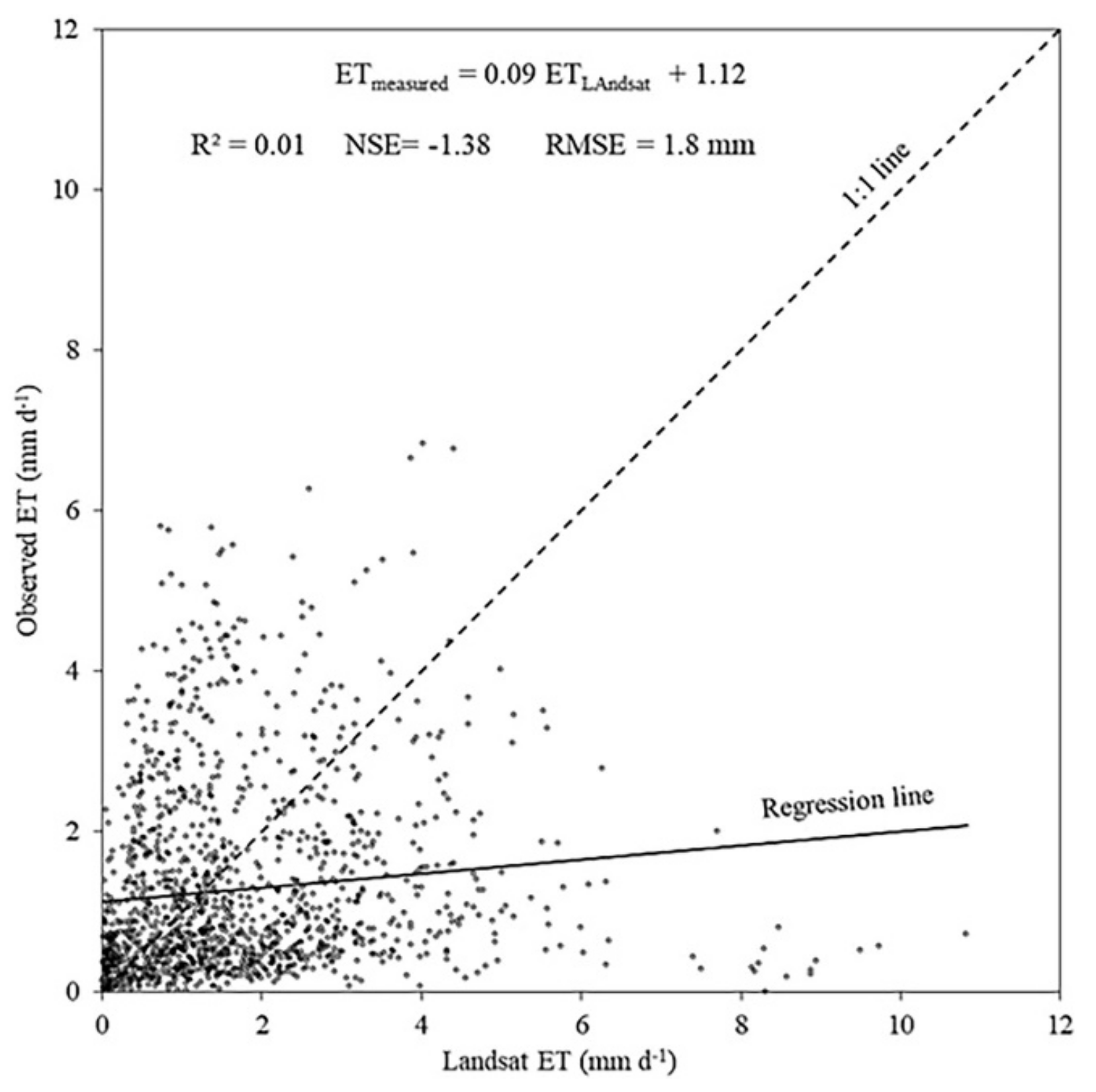
Ten years of lysimeter measured ET data were used in this study. The Landsat-based ET overestimated the measured ET early and late in the growing season and underestimated ET during the peak of the growing season. The daily and monthly ET for the dryland lysimeter was unacceptable with negative NSE (−1.38 and −0.19), indicating there was no correlation between the estimates and measured ET; however, the daily and monthly ET for the irrigated lysimeter values showed better statistics with an NSE of 0.37 and 0.57, respectively. Seasonal ET showed more variations during the growing season compared to the non-growing season, because higher ET values were estimated during the growing season.
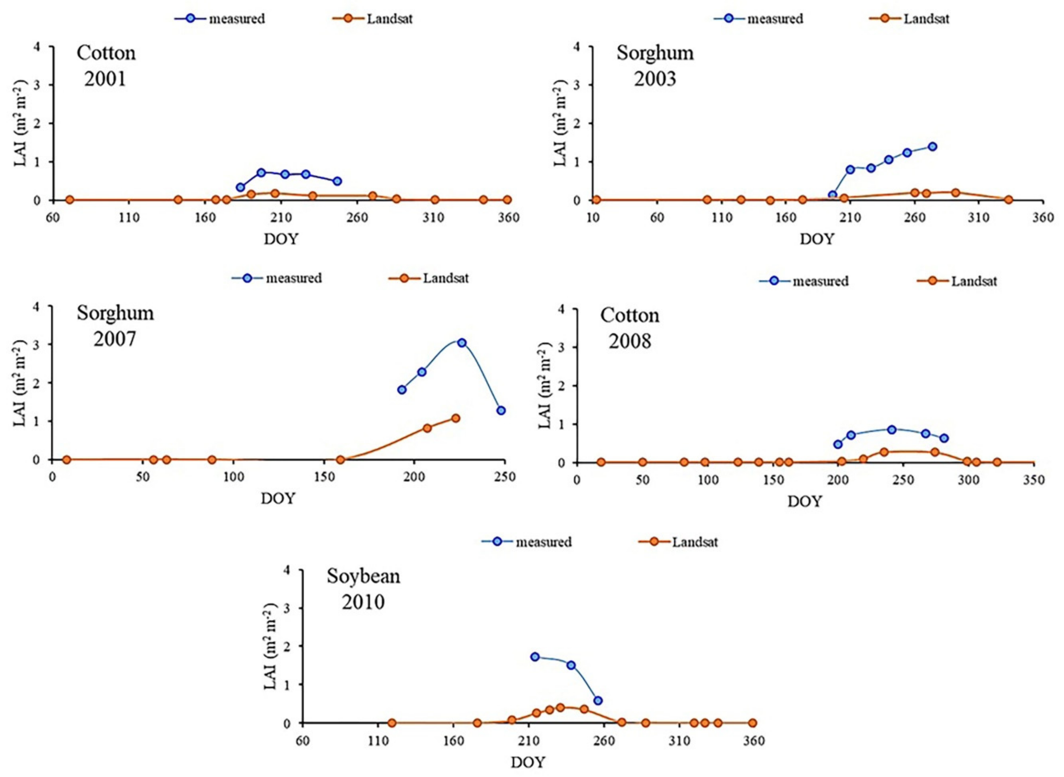
Under dryland conditions, there was significant LAI underestimation compared to the measured LAI values due to water stress during the growing season. LAI plays a significant role in evapotranspiration; where greater values of NDVI were obtained, consequently greater LAI was obtained under irrigated conditions, resulting in more ET for irrigated conditions. There are several reasons behind uncertainties of LAI and ET estimation, including the following: (1) METRIC model uncertainties with partial canopy estimates, (2) dryland plants’ rapid modification of LAI based on available soil water (partial canopy), and (3) uncertainties with aerodynamic resistance surface roughness length as well as surface temperature deviations between irrigated and dryland conditions.
Extended gap periods are another significant challenge, and the selection of the filling method can account for ET estimation errors. In this study, gap periods reached up to 184 days in 2004, and the minimum was in 2008 with 40 days. The linear interpolation method was utilized to extrapolate the daily ET estimates between every two consecutive images in this study.
More satellite-based ET assessment under arid and semi-arid conditions is required, where the magnitude and frequency of precipitation are erratic, and irrigation is the only source under arid conditions to replenish crop water needs. With advances in remote sensing, more frequent satellite imagery will be available, with high spatial resolutions. Other extrapolation methods should be considered to generate daily time-series ET datasets. This would likely improve overall ET estimation accuracy by improving the overall spatial and temporal resolution.
Future research opportunities that include the assessment of ET relationship with crop physiology, yield, and yield components (number of flowers, grain quality, etc.) would provide potential information on crop response under dryland and irrigated conditions. Economic analysis of commodity market prices would be another research project due to groundwater decline in the Ogallala aquifer.

Author Contributions

Writing—original draft, A.A.H.; methodology, A.A.H. and P.H.G.; software, J.E.M., G.W.M., and P.H.G.; resources, B.A.E. and P.H.G.; review and editing, B.A.E., G.W.M., V.F.B., S.A.R., and J.E.M.; supervision, B.A.E. All authors have read and agreed to the published version of the manuscript.

Funding

This research was funded by the Egyptian Government General Mission Scholarship Program administrated by the Egyptian Cultural and Education Bureau, Washington, DC; the Purdue Research Foundation, and the Agricultural and Biological Engineering Department, Purdue University.

Acknowledgments

The authors express their sincere thanks to (1) the Egyptian government general mission scholarship administrated by the Egyptian Cultural and Education Bureau, Washington, DC, for partially supporting this research; (2) the Purdue Research Foundation and the Agricultural and Biological Engineering Department for funding support during this research; and (3) the USDA-ARS at Bushland, Texas, USA for sharing the lysimeter data and data analysis.

Conflicts of Interest

The authors declare no conflict of interest.

References

  1. Sellers, P.J.; Randall, D.A.; Collatz, G.J.; Berry, J.A.; Field, C.B.; Dazlich, D.A.; Zhang, C.; Collelo, G.D.; Bounoua, L. A revised land surface parameterization (SiB2) for atmospheric GCMs. Part I: Model formulation. J. Clim. 1996, 9, 676–705. [Google Scholar] [CrossRef]
  2. Paulson, R.W. Evapotranspiration and Droughts. National Water Summary 1988–1989: Hydrologic Events and Floods and Droughts; US Government Printing Office: Washington, DC, USA, 1991; Volume 2375, pp. 1–147.
  3. Famiglietti, J.S. The global groundwater crisis. Nat. Clim. Chang. 2014, 4, 945–948. [Google Scholar] [CrossRef]
  4. Yaeger, M.A.; Massey, J.H.; Reba, M.L.; Adviento-Borbe, M.A.A. Trends in the construction of on-farm irrigation reservoirs in response to aquifer decline in eastern Arkansas: Implications for conjunctive water resource management. Agric. Water Manag. 2018, 208, 373–383. [Google Scholar] [CrossRef]
  5. Gowda, P.H.; Chávez, J.L.; Colaizzi, P.D.; Evett, S.R.; Howell, T.A.; Tolk, J.A. Remote Sensing Based Energy Balance Algorithms for Mapping ET: Current Status and Future Challenges. Trans. ASABE 2007, 50, 1639–1644. [Google Scholar] [CrossRef]
  6. Allen, R.G.; Tasumi, M.; Morse, A.; Trezza, R.; Wright, J.L.; Bastiaanssen, W.; Kramber, W.; Lorite, I.; Robison, C.W. Satellite-Based Energy Balance for Mapping Evapotranspiration with Internalized Calibration (METRIC)—Applications. J. Irrig. Drain. Eng. 2007, 133, 395–406. [Google Scholar] [CrossRef]
  7. Gowda, P.H.; Chavez, J.L.; Colaizzi, P.D.; Evett, S.R.; Howell, T.A.; Tolk, J.A. ET mapping for agricultural water management: Present status and challenges. Irrig. Sci. 2007, 26, 223–237. [Google Scholar] [CrossRef] [Green Version]
  8. Bastiaanssen, W.; Pelgrum, H.; Wang, J.; Ma, Y.; Moreno, J.; Roerink, G.; van Der Wal, T. A remote sensing surface energy balance algorithm for land (SEBAL). J. Hydrol. 1998, 213–229. [Google Scholar] [CrossRef]
  9. French, A.N.; Hunsaker, D.J.; Thorp, K.R. Remote sensing of evapotranspiration over cotton using the TSEB and METRIC energy balance models. Remote. Sens. Environ. 2015, 158, 281–294. [Google Scholar] [CrossRef]
  10. Park, A.B.; Colwell, R.N.A.; Meyers, V.F. Resource Survey by Satellite; sci-ence fiction coming true. In Yearbook of Agriculture; US Government Printing Office: Washington, DC, USA, 1968; pp. 13–19. [Google Scholar]
  11. Jackson, R.D. Remote Sensing of Vegetation Characteristics for Farm Management. 1984 Tech. Symp. East 1984, 475, 81–97. [Google Scholar] [CrossRef]
  12. Choudhury, B.; Idso, S.; Reginato, R. Analysis of an empirical model for soil heat flux under a growing wheat crop for estimating evaporation by an infrared-temperature based energy balance equation. Agric. For. Meteorol. 1987, 39, 283–297. [Google Scholar] [CrossRef]
  13. Su, H.; McCabe, M.; Wood, E.F.; Su, Z.; Prueger, J.H. Modeling Evapotranspiration during SMACEX: Comparing Two Approaches for Local- and Regional-Scale Prediction. J. Hydrometeorol. 2005, 6, 910–922. [Google Scholar] [CrossRef]
  14. Anderson, M.C.; Kustas, W.P.; Norman, J.M.; Hain, C.R.; Mecikalski, J.R.; Schultz, L.; González-Dugo, M.P.; Cammalleri, C.; D’Urso, G.; Pimstein, A.; et al. Mapping daily evapotranspiration at field to continental scales using geostationary and polar orbiting satellite imagery. Hydrol. Earth Syst. Sci. 2011, 15, 223–239. [Google Scholar] [CrossRef] [Green Version]
  15. Evett, S.R.; Kustas, W.P.; Gowda, P.H.; Anderson, M.C.; Prueger, J.H.; Howell, T.A. Overview of the Bushland Evapotranspiration and Agricultural Remote sensing EXperiment 2008 (BEAREX08): A field experiment evaluating methods for quantifying ET at multiple scales. Adv. Water Resour. 2012, 50, 4–19. [Google Scholar] [CrossRef]
  16. Bastiaanssen, W.G.M.; Noordman, E.J.M.; Pelgrum, H.; Davids, G.; Thoreson, B.P.; Allen, R. SEBAL Model with Remotely Sensed Data to Improve Water-Resources Management under Actual Field Conditions. J. Irrig. Drain. Eng. 2005, 131, 85–93. [Google Scholar] [CrossRef]
  17. Tasumi, M.; Allen, R.G. Satellite-based ET mapping to assess variation in ET with timing of crop development. Agric. Water Manag. 2007, 88, 54–62. [Google Scholar] [CrossRef]
  18. Norman, J.; Kustas, W.; Humes, K. Source approach for estimating soil and vegetation energy fluxes in observations of directional radiometric surface temperature. Agric. For. Meteorol. 1995, 77, 263–293. [Google Scholar] [CrossRef]
  19. Colaizzi, P.D.; Evett, S.R.; Howell, T.A.; Gowda, P.H.; Shaughnessy, S.A.; Tolk, J.A.; Kustas, W.P.; Anderson, M.C. Two-Source Energy Balance Model: Refinements and Lysimeter Tests in the Southern High Plains. Trans. ASABE 2012, 55, 551–562. [Google Scholar] [CrossRef]
  20. Kustas, W.P.; Norman, J.M. Evaluation of soil and vegetation heat flux predictions using a simple two-source model with radiometric temperatures for partial canopy cover. Agric. For. Meteorol. 1999, 94, 13–29. [Google Scholar] [CrossRef]
  21. Kalma, J.D.; McVicar, T.R.; Matthew, F. UNSW Faculty of Engineering Matthew Francis McCabe Estimating Land Surface Evaporation: A Review of Methods Using Remotely Sensed Surface Temperature Data. Surv. Geophys. 2008, 29, 421–469. [Google Scholar] [CrossRef]
  22. Moorhead, J.E.; Marek, G.W.; Gowda, P.H.; Lin, X.; Colaizzi, P.D.; Evett, S.R.; Kutikoff, S. Evaluation of Evapotranspiration from Eddy Covariance Using Large Weighing Lysimeters. Agronomy 2019, 9, 99. [Google Scholar] [CrossRef] [Green Version]
  23. Anderson, M.; Norman, J.; Kustas, W.; Houborg, R.; Starks, P.; Agam, N. A thermal-based remote sensing technique for routine mapping of land-surface carbon, water and energy fluxes from field to regional scales. Remote Sens. Environ. 2008, 112, 4227–4241. [Google Scholar] [CrossRef]
  24. Marek, T.H.; Schneider, A.D.; Howell, T.A.; Ebeling, L.L. Design and Construction of Large Weighing Monolithic Lysimeters. Trans. ASAE 1988, 31, 477–484. [Google Scholar] [CrossRef]
  25. Howell, T.A.; Schneider, A.D.; Dusek, D.A.; Marek, T.H.; Steiner, J.L. Calibration and Scale Performance of Bushland Weighing Lysimeters. Trans. ASAE 1995, 38, 1019–1024. [Google Scholar] [CrossRef]
  26. Norman, J.M.; Anderson, M.C.; Kustas, W.P.; French, A.N.; Mecikalski, J.; Torn, R.; Diak, G.R.; Schmugge, T.J.; Tanner, B.C.W. Remote sensing of surface energy fluxes at 101-m pixel resolutions. Water Resour. Res. 2003, 39, 39. [Google Scholar] [CrossRef] [Green Version]
  27. Anderson, M.C.; Norman, J.M.; Mecikalski, J.R.; Otkin, J.A.; Kustas, W.P. A climatological study of evapotranspiration and moisture stress across the continental United States based on thermal remote sensing: 2. Surface moisture climatology. J. Geophys. Res. Space Phys. 2007, 112, 112. [Google Scholar] [CrossRef]
  28. Anderson, M.; Kustas, W.P.; Norman, J.M. Upscaling Flux Observations from Local to Continental Scales Using Thermal Remote Sensing. Agron. J. 2007, 99, 240–254. [Google Scholar] [CrossRef] [Green Version]
  29. Colaizzi, P.D.; Evett, S.R.; Howell, T.A.; Tolk, J.A. Comparison of Five Models to Scale Daily Evapotranspiration from One-Time-of-Day Measurements. Trans. ASABE 2006, 49, 1409–1417. [Google Scholar] [CrossRef]
  30. Allen, R.G.; Pereira, L.S.; Howell, T.A.; Jensen, M.E. Evapotranspiration information reporting: I. Factors governing measurement accuracy. Agric. Water Manag. 2011, 98, 899–920. [Google Scholar] [CrossRef] [Green Version]
  31. Allen, R.G.; Pereira, L.S.; Howell, T.A.; Jensen, M.E. Evapotranspiration information reporting: II. Recommended documentation. Agric. Water Manag. 2011, 98, 921–929. [Google Scholar] [CrossRef]
  32. Chávez, J.L.; Gowda, P.H.; Howell, T.A.; Garcia, L.A.; Copeland, K.S.; Neale, C.M.U. ET Mapping with High-Resolution Airborne Remote Sensing Data in an Advective Semiarid Environment. J. Irrig. Drain. Eng. 2012, 138, 416–423. [Google Scholar] [CrossRef]
  33. Mkhwanazi, M.; Chávez, J.L.; Rambikur, E.H. Comparison of Large Aperture Scintillometer and Satellite-based Energy Balance Models in Sensible Heat Flux and Crop Evapotranspiration Determination. Int. J. Remote Sens. Appl. 2012, 2, 24. [Google Scholar]
  34. Morton, C.G.; Huntington, J.L.; Pohll, G.M.; Allen, R.G.; McGwire, K.C.; Bassett, S.D. Assessing Calibration Uncertainty and Automation for Estimating Evapotranspiration from Agricultural Areas Using METRIC. JAWRA J. Am. Water Resour. Assoc. 2013, 49, 549–562. [Google Scholar] [CrossRef]
  35. Trezza, R.; Allen, R.; Tasumi, M. Estimation of Actual Evapotranspiration along the Middle Rio Grande of New Mexico Using MODIS and Landsat Imagery with the METRIC Model. Remote Sens. 2013, 5, 5397–5423. [Google Scholar] [CrossRef] [Green Version]
  36. Chávez, J.L.; Gowda, P.H.; Howell, T.A.; Copeland, K.S. Evaluating Three Evapotranspiration Mapping Algorithms with Lysimetric Data in the Semi-arid Texas High Plains. In Proceedings of the 28th annual international irrigation show, San Diego, CA, USA, 9–11 December 2007. [Google Scholar]
  37. Dusek, D.A.; Howell, T.A.; Schneider, A.D.; Copeland, K.S. Bushland weighing lysimeter data acquisition systems for evapotranspiration research. Am. Soc. Agric. Eng. 1987, 1061, 81–2506. [Google Scholar]
  38. Hashem, A.A. Irrigation Water Management Using Remote Sensing and Hydrologic Modeling. Ph.D. Thesis, Purdue University, West Lafayette, IN, USA, 2018. [Google Scholar]
  39. Marek, G.W.; Gowda, P.; Evett, S.R.; Baumhardt, R.L.; Brauer, D.; Howell, T.A.; Marek, T.H.; Srinivasan, R. Calibration and Validation of the SWAT Model for Predicting Daily ET over Irrigated Crops in the Texas High Plains Using Lysimetric Data. Trans. ASABE 2016, 59, 611–622. [Google Scholar] [CrossRef] [Green Version]
  40. Marek, G.W.; Gowda, P.; Evett, S.R.; Baumhardt, R.L.; Brauer, D.K.; Howell, T.A.; Marek, T.H.; Srinivasan, R. Estimating Evapotranspiration for Dryland Cropping Systems in the Semiarid Texas High Plains Using SWAT. JAWRA J. Am. Water Resour. Assoc. 2016, 52, 298–314. [Google Scholar] [CrossRef]
  41. Hashem, A.A.; Engel, B.; Bralts, V.F.; Marek, G.W.; Moorhead, J.E.; Rashad, M.; Radwan, S.; Gowda, P.H. Landsat Hourly Evapotranspiration Flux Assessment using Lysimeters for the Texas High Plains. Water 2020, 12, 1192. [Google Scholar] [CrossRef]
  42. Moorhead, J.E.; Gowda, P.H.; Ponder, B.A.; Brauer, D.K. Bushland Evapotranspiration and Agricultural Remote Sensing System (BEARS) software. In Proceedings of the Managing Global Resources for a Secure Future, Tampa, FL, USA, 22–25 October 2017. [Google Scholar]
  43. Allen, R.G.; Pereira, L.S.; Raes, D.; Smith, M. Crop Evapotranspiration—Guidelines for Computing Crop Water Requirements; FAO Irrigation and Drainage Paper 56: Rome, Italy, 1998; ISBN 92-5-104219-5. [Google Scholar]
  44. Blonquist, J.; Allen, R.; Bugbee, B. An evaluation of the net radiation sub-model in the ASCE standardized reference evapotranspiration equation: Implications for evapotranspiration prediction. Agric. Water Manag. 2010, 97, 1026–1038. [Google Scholar] [CrossRef]
  45. Allen, R.G.; Burnett, B.; Kramber, W.; Huntington, J.L.; Kjaersgaard, J.; Kilic, A.; Kelly, C.; Trezza, R. Automated Calibration of the METRIC-Landsat Evapotranspiration Process. JAWRA J. Am. Water Resour. Assoc. 2013, 49, 563–576. [Google Scholar] [CrossRef]
  46. Allen, R.G.; Irmak, A.; Trezza, R.; Hendrickx, J.M.H.; Bastiaanssen, W.G.M.; Kjaersgaard, J. Satellite-based ET estimation in agriculture using SEBAL and METRIC. Hydrol. Process. 2011, 25, 4011–4027. [Google Scholar] [CrossRef]
  47. Hashem, A.A.; Engel, B.A.; Marek, G.W.; Moorhead, J.E.; Rashad, M.; Flanagan, D.C.; Radwan, S.; Bralts, V.F.; Gowda, P.H. Evaluation of SWAT Soil Water Estimation Accuracy Using Data from Indiana, Colorado, and Texas. Trans. ASABE 2020, 5, 1539–1559. [Google Scholar]
  48. Moriasi, D.N.; Arnold, J.G.; van Liew, M.W.; Bingner, R.L.; Harmel, R.D.; Veith, T.L. Model Evaluation Guidelines for Systematic Quantification of Accuracy in Watershed Simulations. Trans. ASABE 2007, 50, 885–900. [Google Scholar] [CrossRef]
  49. Madugundu, R.; Al-Gaadi, K.A.; Tola, E.; Hassaballa, A.A.; Patil, V.C. Performance of the METRIC model in estimating evapotranspiration fluxes over an irrigated field in Saudi Arabia using Landsat-8 images. Hydrol. Earth Syst. Sci. 2017, 21, 6135–6151. [Google Scholar] [CrossRef] [Green Version]
  50. Senay, G.B.; Friedrichs, M.; Singh, R.K.; Velpuri, N.M. Evaluating Landsat 8 evapotranspiration for water use mapping in the Colorado River Basin. Remote Sens. Environ. 2016, 185, 171–185. [Google Scholar] [CrossRef] [Green Version]
  51. Moorhead, J.E.; Marek, G.W.; Colaizzi, P.D.; Gowda, P.; Evett, S.R.; Brauer, D.; Marek, T.H.; Porter, D.O. Evaluation of Sensible Heat Flux and Evapotranspiration Estimates Using a Surface Layer Scintillometer and a Large Weighing Lysimeter. Sensors 2017, 17, 2350. [Google Scholar] [CrossRef] [PubMed] [Green Version]
  52. Gowda, P.H.; Howell, T.A.; Paul, G.; Colaizzi, P.D.; Marek, T.H.; Su, Z.; Copeland, K.S. Deriving Hourly Evapotranspiration Rates with SEBS: A Lysimetric Evaluation. Vadose Zone J. 2013, 12, 1–11. [Google Scholar] [CrossRef] [Green Version]
  53. Numata, I.; Khand, K.; Kjaersgaard, J.; Cochrane, M.A.; Silva, S.S. Evaluation of Landsat-Based METRIC Modeling to Provide High-Spatial Resolution Evapotranspiration Estimates for Amazonian Forests. Remote Sens. 2017, 9, 46. [Google Scholar] [CrossRef] [Green Version]
Figure 1. Daily and seven-day running average measured and Landsat evapotranspiration (ET) from (a) 2001–2005, and (b) 2006–2010 for the northwest (NW) dryland lysimeter. The years 2004 and 2007 had limited clear remote sensing observations during the growing season.
Agronomy 10 01688 g001
Figure 2. Daily 1:1 graph of measured and Landsat ET for NW dryland lysimeter. The years 2004 and 2007 were omitted from the analysis due to limited clear image availability.
Agronomy 10 01688 g002
Figure 3. Monthly average measured and Landsat ET for the NW dryland lysimeter. The years 2004 and 2007 had limited clear remote sensing observations during the growing season.
Agronomy 10 01688 g003
Figure 4. Measured and calculated Landsat leaf area index (LAI) for the NW dryland lysimeter. The year 2004 graph omitted because Landsat LAI values were not available.
Agronomy 10 01688 g004
Figure 5. Daily and seven-day running average measured and calculated Landsat ET from (a) 2001–2005, and (b) 2006–2010 for the northeast (NE) irrigated lysimeter. The years 2004 and 2007 had limited clear remote sensing observations during the growing season.
Agronomy 10 01688 g005
Figure 6. Daily 1:1 graph of measured and Landsat ET for the NE irrigated lysimeter. The years 2004 and 2007 were omitted from the analysis due to limited clear image availability.
Agronomy 10 01688 g006
Figure 7. Monthly average measured and Landsat estimated ET for the NE irrigated lysimeter. The years 2004 and 2007 had limited clear remote sensing observations during the growing season.
Agronomy 10 01688 g007
Figure 8. Measured and Landsat leaf area index (LAI) for the NE irrigated lysimeter. The year 2004 graph omitted because Landsat LAI values were not available.
Agronomy 10 01688 g008
Table 1. Landsat image dates and corresponding day of year (DOY).
2001 (Cotton-Limited Irrigation)2002 (Cotton-Limited Irrigation)2003 (Soybean)2004 (Soybean)2005 (Sorghum)2006 (Forage Corn)2007 (Forage Sorghum)2008 (Cotton)2009 (Sunflower)2010 (Cotton)
#Date (DOY)Date (DOY)Date (DOY)Date (DOY)Date (DOY)Date (DOY)Date (DOY)Date (DOY)Date (DOY)Date (DOY)
1March 12 (71)January 26
(26)
January 13 (13)February 17 (48)January 25 (25)January 18 (28)January 8 (8)January 18 (18)January 13 (13)April 29 (119)
2May,22 (142)February 11 (42)April 10 (100)March 20 (80)February 3 (34)February 13 (44)February 25 (56)February 19 (50)January 20 (20)June 25 (176)
3June 16 (167)March 3 (90)May 5 (125)March 27 (87)March 7 (66)April 18 (108)March 4 (63)March 22 (82)January 29 (29)July 18 (199)
4June 23 (174)May 9 (129)May 28 (148)April 21 (112)June 18 (169)May 20 (140)March 29 (88)April 7 (95)February 5 (36)August 3 (215)
5July 9 (190)May 18 (138)June 24 (205)May 14 (135)June 27 (178)June 5 (156)June 8 (159)May 2 (123)February 21 (52)August 12 (224)
6July 25 (206)June 10 (161)July 17 (198)May 30 (151)July 20 (201)July 23 (204)July 26 (207)May 18 (139)March 18 (77)August 19 (231)
7August 19 (231)June 19 (170)September 17 (260)December 1 (336)August 30 (242)August 8 (220)August 11 (223)June 3 (155)April 3 (93)September 4 (247)
8September 27 (270)July 21 (202)September 26 (269)December 12 (352)September 22 (265)August 24 (236) June 10 (162)June 22 (173)September 29 (272)
9October 13 (286)September 23 (266)October 19 (292) October 1 (274)September 18 (261) July 21 (203)July 8 (189)October 15 (288)
10November 7 (311) November 29 (333) October 24 (297)September 25 (268) August 6 (219)August 16 (228)November 16 (320)
11December 9 (343) November 18 (315)October 11 (284) August 22 (235)November 4 (308)November 23 (327)
12December 12 (359) October 27 (300) September 30 (274)November 20 (324)December 12 (355)
13 November 28 (332) October 25 (299) December 25 (359)
14 November 1 (306)
15 November 17 (322)
16 December 28 (363)
Table 2. Average frequency and maximum gap each year for the study site.
YearAverage Frequency (Days)Maximum Gap (Days)Dates of Maximum Gap DOY of Maximum Gap
20013070March 12–May 22DOY 71 To DOY 142
20024199September 23–December 31DOY 266 To DOY 365
20033786January 13–April 10DOY 13 To DOY 100
200446184May 30–December 1DOY 151 To DOY 336
200533102March 7–June 18DOY 66 To DOY 169
20062863February 13–April 18DOY 44 To DOY 108
200752141August 19–December 31DOY 231 To DOY 365
20082340June 10–July 21DOY 162 To DOY 203
20093056August 16–November 11DOY 228 To DOY 315
201028118January 1–April 29DOY 1 To DOY 119
The years 2004 and 2007 were omitted from the analysis due to limited clear image availability. Day of the year (DOY).
Table 3. Hot and cold pixel conditions.
PixelConstraintCondition
TsNDVI
Hot (dry)High≤0.2Bare agricultural soil
Cold (Wet)Low≥0.7Cultivated agricultural soil
Table 4. Daily and monthly summary statistics for the NW dryland lysimeter with Landsat ET.
DailyMonthly
R M S E (mm)1.81.2
% R M S E error144.3105.7
N S E −1.38−0.19
Measured average ET (mm d−1)1.31.1
Landsat average ET (mm d−1)1.71.4
RegressionR20.01-
Slope0.09-
Table 5. Seasonal summary statistics for the NW dryland lysimeter with Landsat ET.
Crop RMSE (mm)% RMSE ErrorMeasured Average ET (mm d−1)Landsat Average ET (mm d−1)
Cotton2001 GS1.783.42.01.1
2001 NG1.2123.10.90.9
Fallow2002 GS----
2002 NG2.5288.40.92.0
Sorghum2003 GS1.971.42.71.7
2003 NG1.4171.00.81.5
Fallow2005 GS----
2005 NG1.7143.61.22.0
Sorghum2006 GS1.348.92.72.6
2006 NG0.8104.50.80.7
Cotton2008 GS1.870.52.52.6
2008 NG1.5177.60.81.4
Fallow2009 GS----
2009 NG1.8144.31.21.
Soybean2010 GS3.399.13.32.0
2010 NG2.2215.91.02.0
GS: growing season, NG: non-growing season. The years 2004 and 2007 were omitted from the analysis due to limited clear image availability.
Table 6. Daily and monthly summary statistics for the NE irrigated lysimeter with Landsat ET.
DailyMonthly
RMSE (mm)2.11.5
% RMSE error86.456.7
NSE0.370.57
Measured average ET (mm d−1)2.41.9
Landsat average ET (mm d−1)2.41.9
RegressionR20.38-
Slope0.86-
The years 2004 and 2007 were omitted from the statistical analysis due to limited clear image availability.
Table 7. Seasonal summary statistics for the NE irrigated lysimeter with Landsat ET.
Crop RMSE (mm)%RMSE ErrorMeasured Average ET (mm d−1)Landsat Average ET (mm d−1)
Cotton2001 GS2.066.23.12.1
2001 NG1.4132.11.10.5
Cotton2002 GS3.581.94.24.0
2002 NG1.8156.31.11.9
Soybean2003 GS2.755.24.94.0
2003 NG1.4156.00.91.8
Sorghum2005 GS1.853.43.43.6
2005 NG1.1114.21.01.3
Forage corn2006 GS2.762.34.33.1
2006 NG1.3138.40.90.9
Cotton2008 GS2.756.14.93.3
2008 NG1.8186.90.91.8
Sunflower2009 GS3.975.75.13.8
2009 NG1.4139.90.91.4
Cotton2010 GS3.587.83.93.9
2010 NG1.8185.50.91.8
GS: growing season, NG: non-growing season. The years 2004 and 2007 were omitted from the analysis due to limited clear image availability.
Publisher’s Note: MDPI stays neutral with regard to jurisdictional claims in published maps and institutional affiliations.

