
Crosslinking Rapidly Cured Epoxy Resin Thermosets: Experimental and Computational Modeling and Simulation Study
 , , ,
, , ,
Abstract
:
1. Introduction
2. Materials and Methods
2.1. Materials
Sample Preparation
2.2. Methods
2.2.1. Experimental Work
- Phase behavior and thermo-mechanical properties:
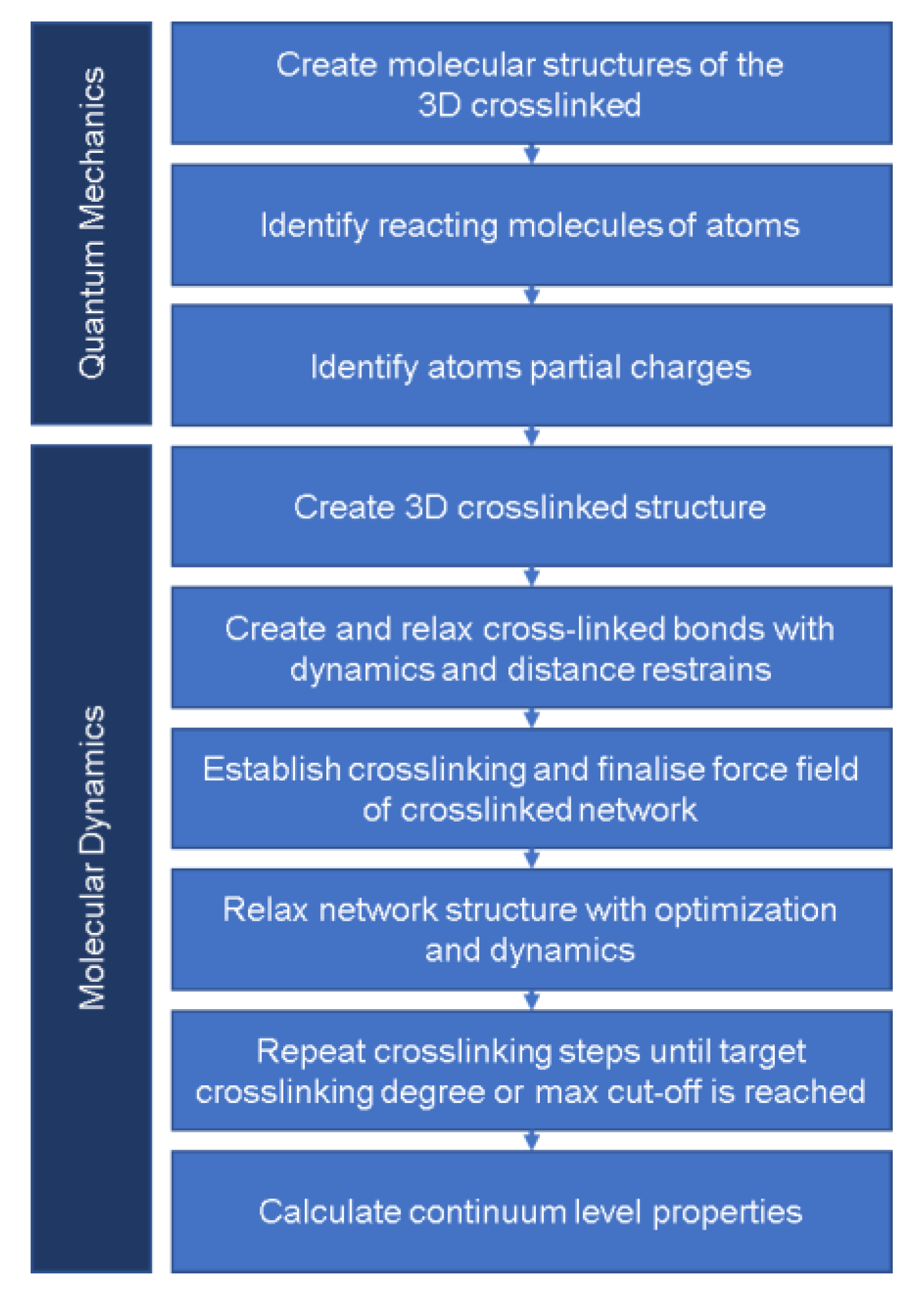
2.2.2. Protocol
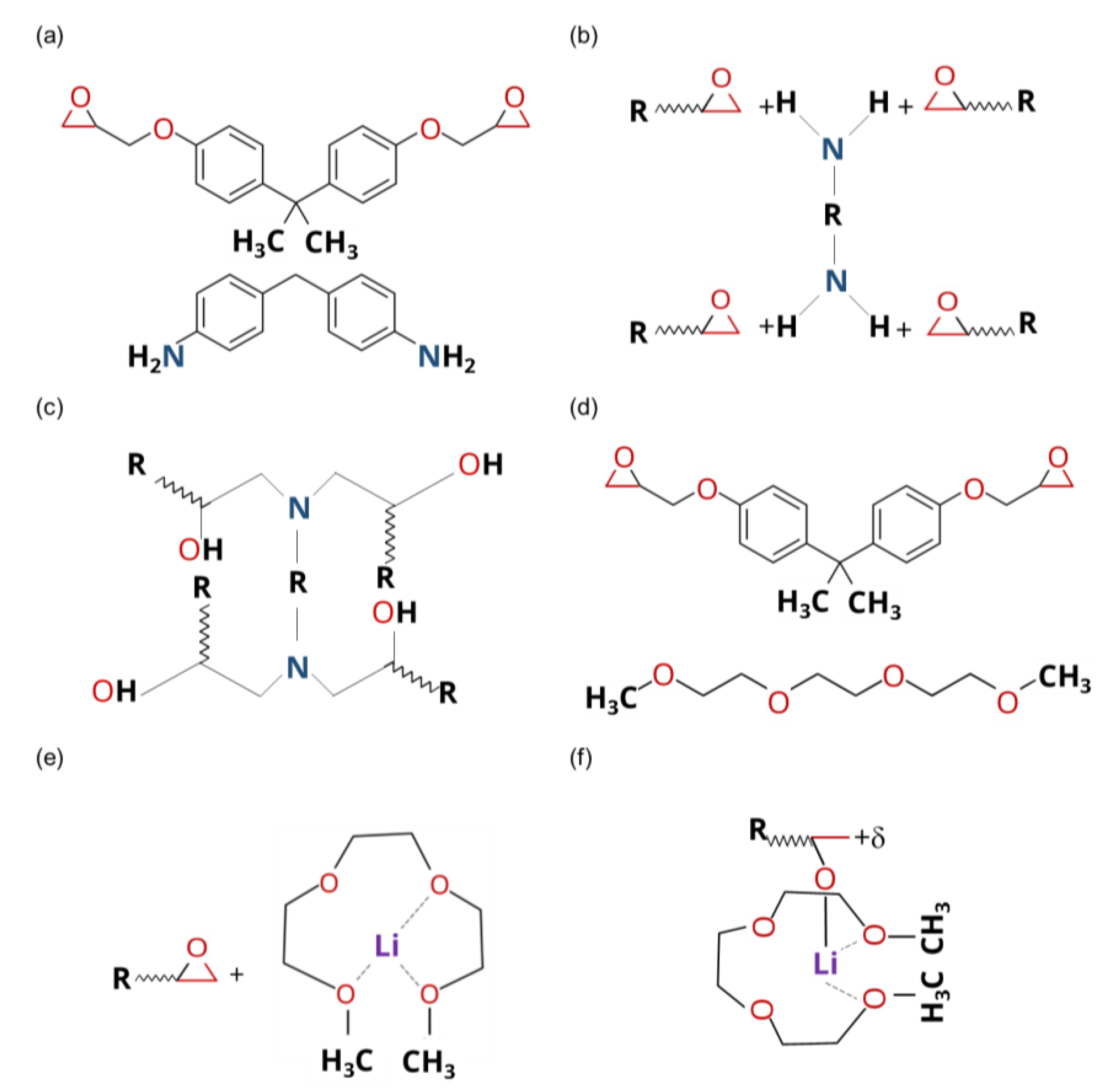
- Atomic Structure
- Reacting Molecules
- Partial Charges
- 3D Structure
- 3D Equilibrated and Crosslinked Structures
- 3D Crosslinking Procedure
- Prediction of Continuum-Level Properties
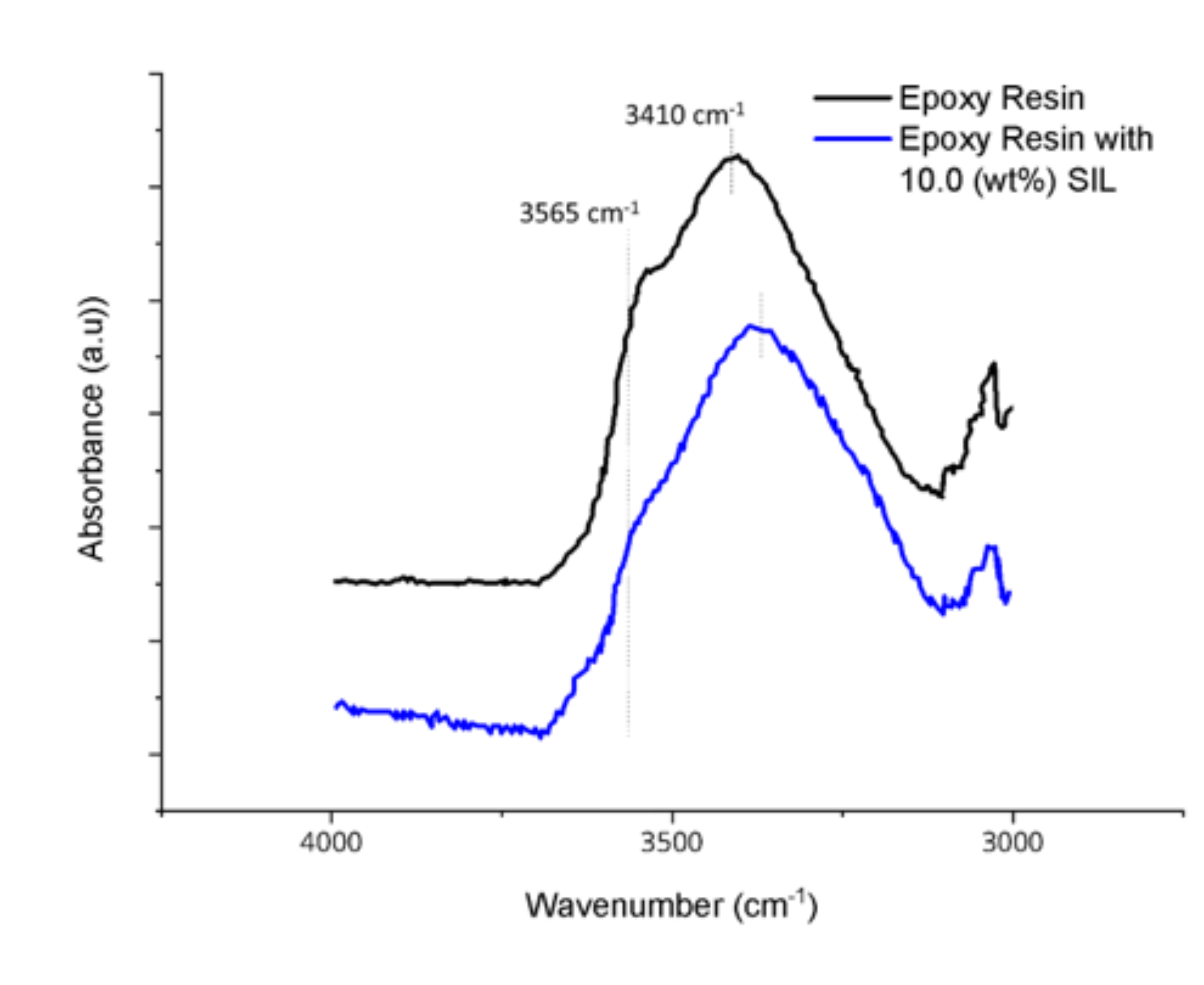
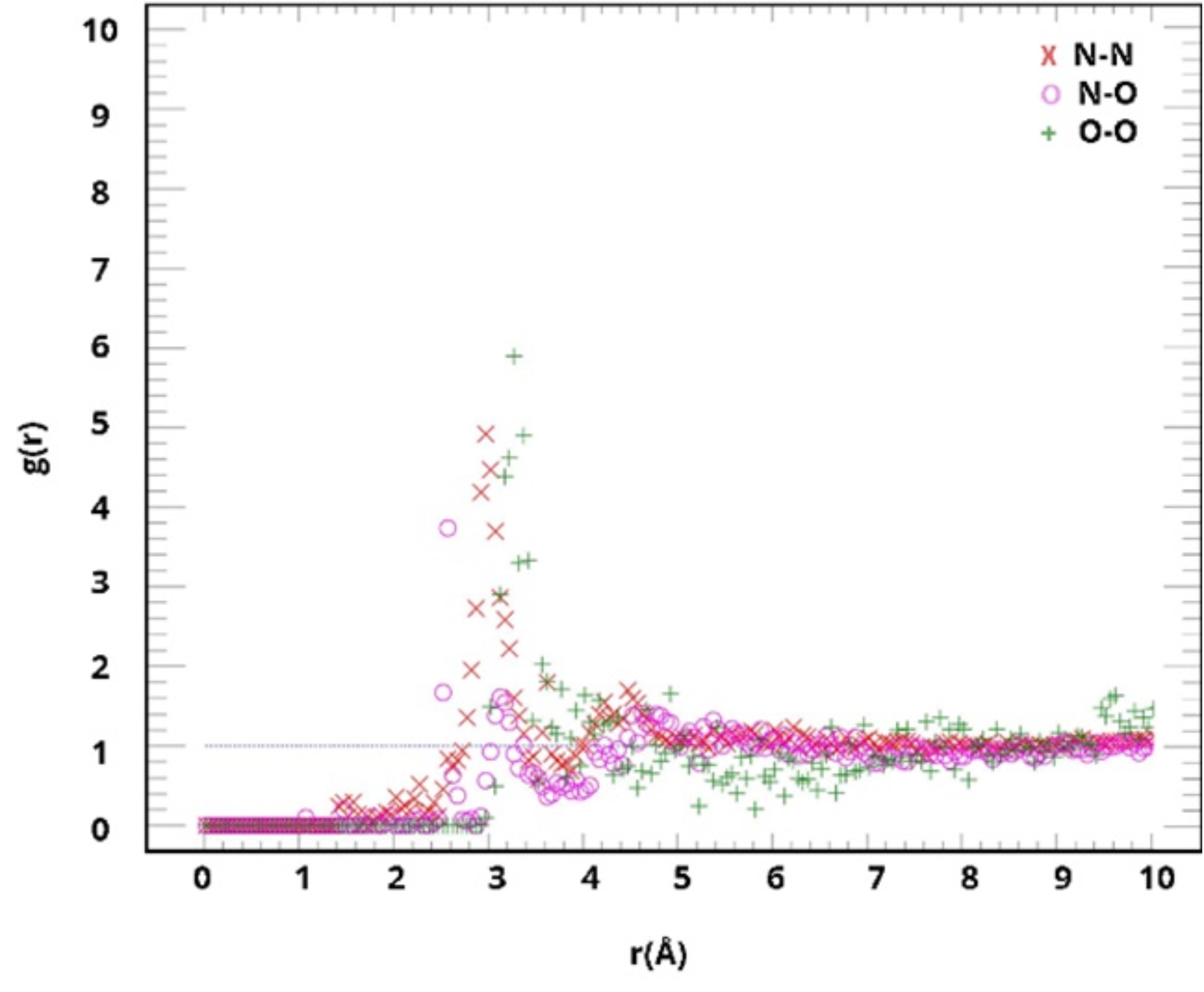
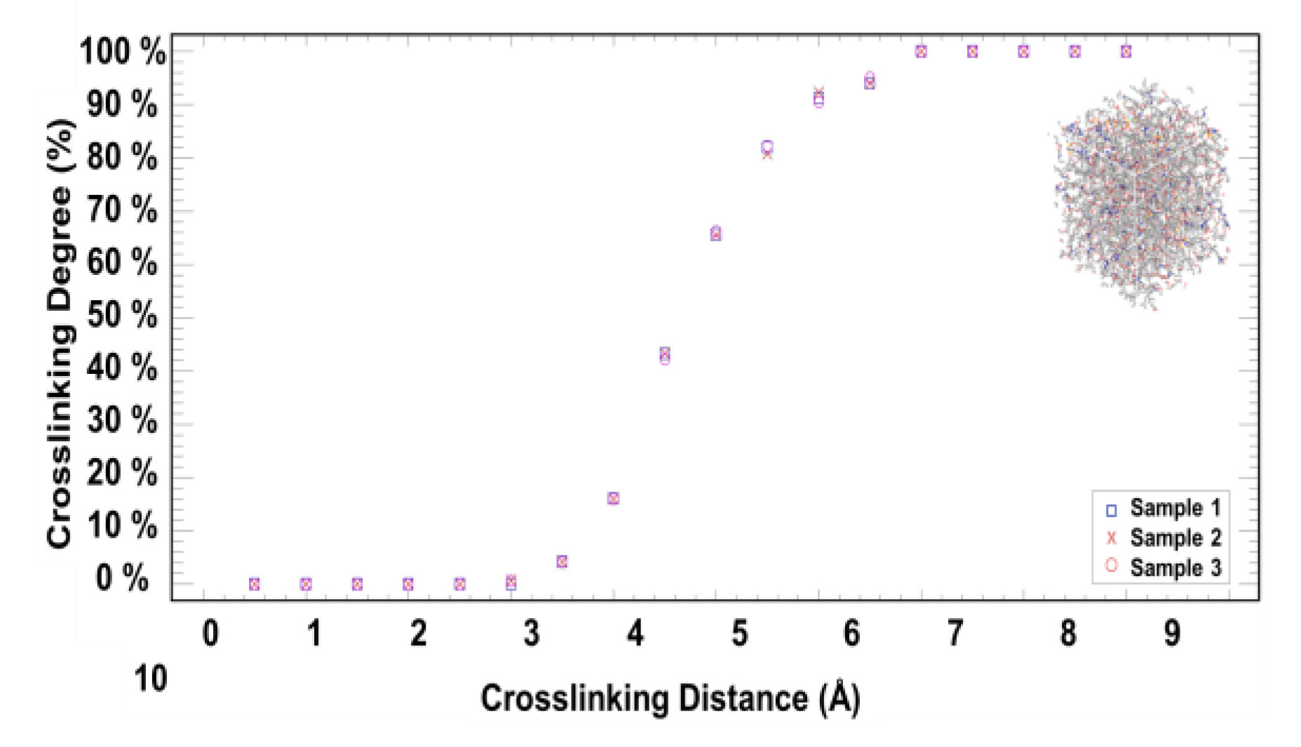
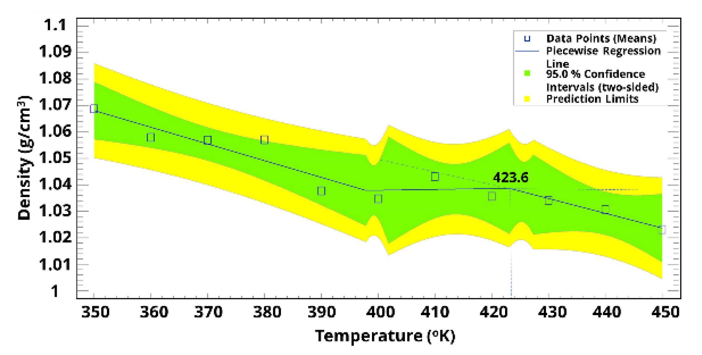
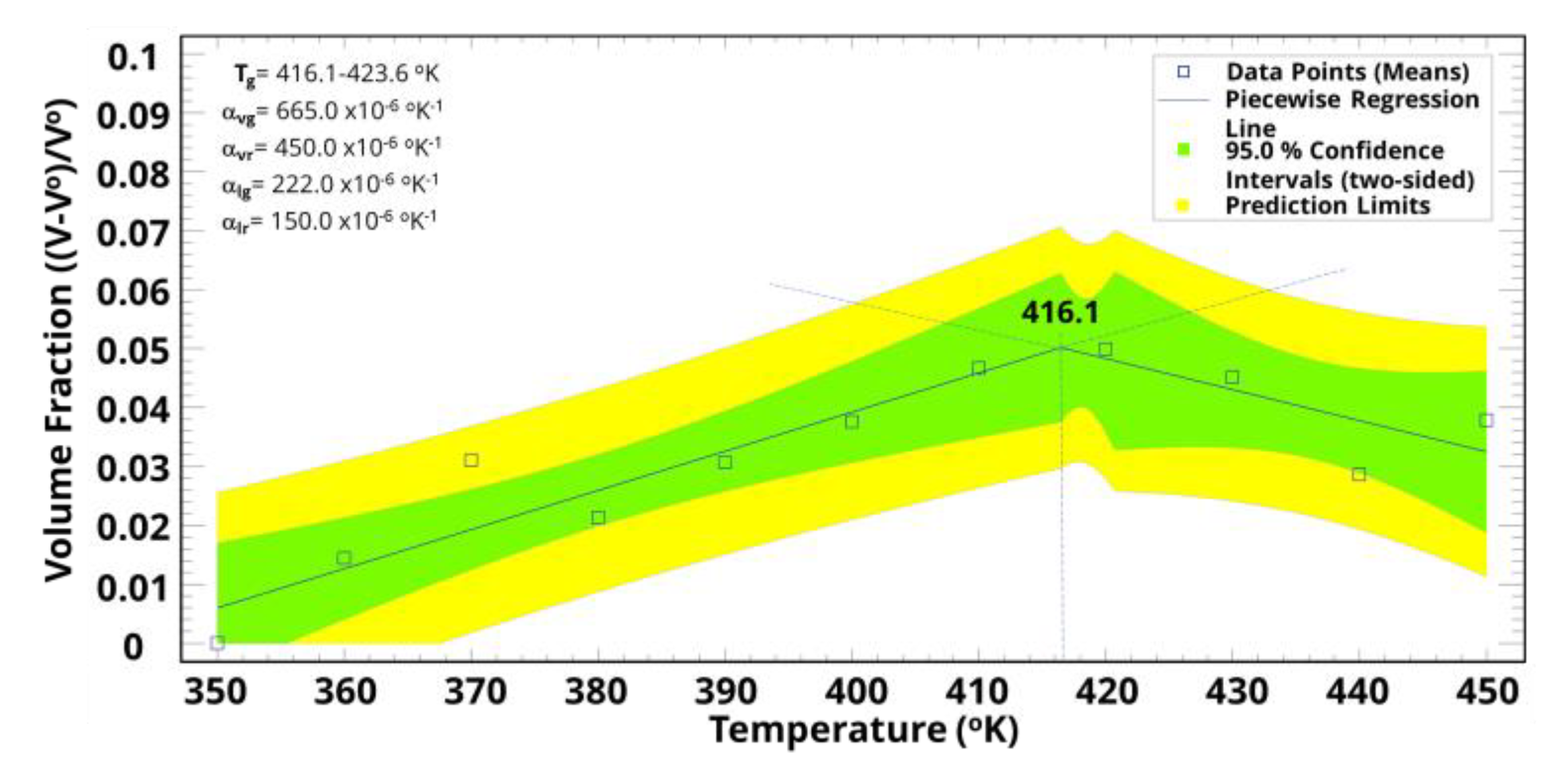
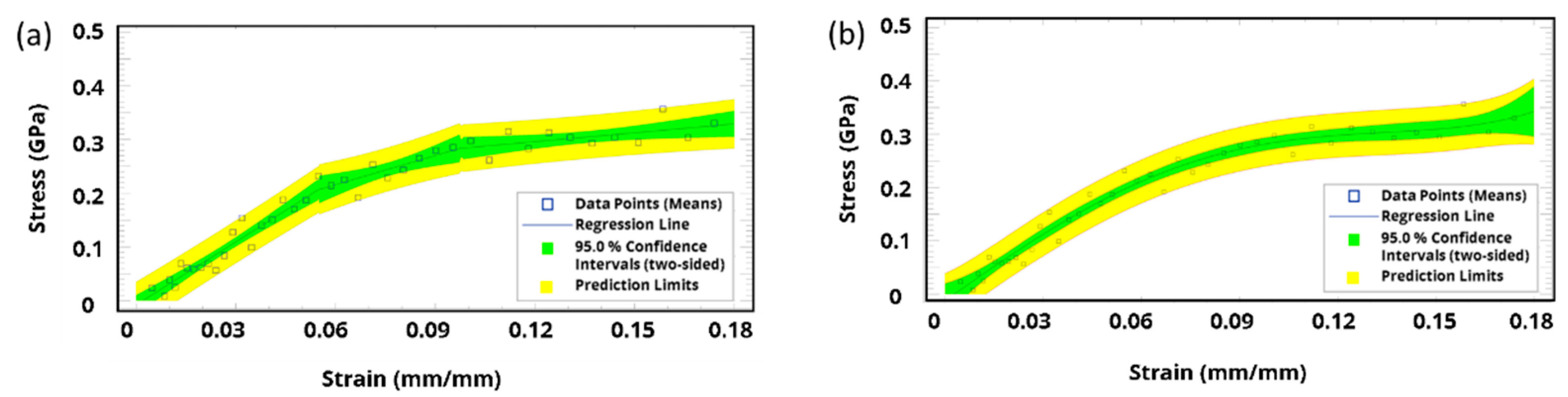
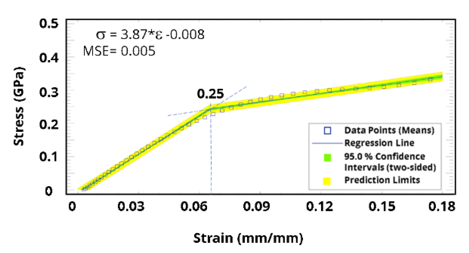
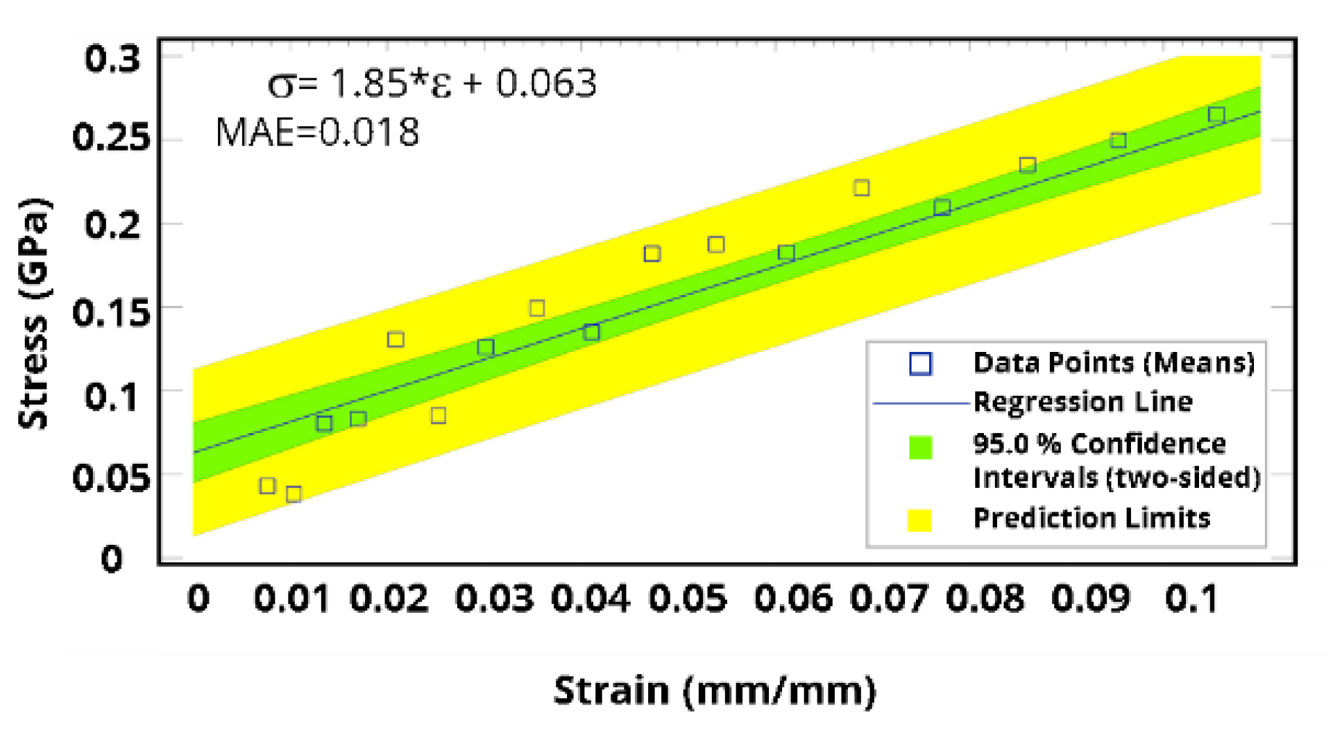
3. Results and Discussion

4. Conclusions
Supplementary Materials
Author Contributions
Funding
Institutional Review Board Statement
Data Availability Statement
Acknowledgments
Conflicts of Interest
References
- Hameed, N.; Eyckens, D.J.; Long, B.M.; Salim, N.V.; Capricho, J.C.; Servinis, L.; De Souza, M.; Perus, M.D.; Varley, R.J.; Henderson, L.C. Rapid Crosslinking of Epoxy Thermosets Induced by Solvate Ionic Liquids. ACS Appl. Polym. Mater. 2020, 2, 2651–2657. [Google Scholar] [CrossRef]
- Odom, M.G.B.; Sweeney, C.B.; Parviz, D.; Sill, L.P.; Saed, M.A.; Green, M.J. Rapid curing and additive manufacturing of thermoset systems using scanning microwave heating of carbon nanotube/epoxy composites. Carbon 2017, 120, 447–453. [Google Scholar] [CrossRef]
- Li, C.; Strachan, A. Molecular scale simulations on thermoset polymers: A review. J. Polym. Sci. Part B Polym. Phys. 2015, 53, 103–122. [Google Scholar] [CrossRef]
- Jang, C.; Sirk, T.W.; Andzelm, J.W.; Abrams, C.F. Comparison of Crosslinking Algorithms in Molecular Dynamics Simulation of Thermosetting Polymers. Macromol. Theory Simul. 2015, 24, 260–270. [Google Scholar] [CrossRef]
- Krausse, C.A.; Milek, T.; Zahn, D. Molecular modeling of amorphous, non-woven polymer networks. J. Mol. Model. 2015, 21, 263. [Google Scholar] [CrossRef] [PubMed]
- Xin, D.R.; Han, Q. Molecular dynamics study on the tensile deformation of crosslinking epoxy resin. J. Mol. Model. 2015, 21, 5. [Google Scholar] [CrossRef] [PubMed]
- Wu, J.; Shi, Q.; Zhang, Z.; Wu, H.H.; Wang, C.; Ning, F.; Xiao, S.; He, J.; Zhang, Z. Nature-inspired entwined coiled carbon mechanical metamaterials: Molecular dynamics simulations. Nanoscale 2018, 10, 15641–15653. [Google Scholar] [CrossRef] [Green Version]
- Araki, M.; Matsumoto, S.; Bekker, G.J.; Isaka, Y.; Sagae, Y.; Kamiya, N.; Okuno, Y. Exploring ligand binding pathways on proteins using hypersound-accelerated molecular dynamics. Nat. Commun. 2021, 12, 2793. [Google Scholar] [CrossRef]
- Hospital, A.; Goni, J.R.; Orozco, M.; Gelpi, J.L. Molecular dynamics simulations: Advances and applications. Adv. Appl. Bioinform. Chem. 2015, 8, 37–47. [Google Scholar] [CrossRef] [Green Version]
- The PLUMED Consortium. Promoting transparency and reproducibility in enhanced molecular simulations. Nat. Methods 2019, 16, 670–673. [Google Scholar] [CrossRef] [Green Version]
- Li, J.; Guo, P.; Kong, X.; Wang, Y.; Li, F.; Du, B. Curing Degree Dependence of Dielectric Properties of Bisphenol-A-Based Epoxy Resin Cured With Methyl Hexahydrophthalic Anhydride. IEEE Trans. Dielectr. Electr. Insul. 2022, 29, 2072–2079. [Google Scholar] [CrossRef]
- Peerless, J.S.; Kwansa, A.L.; Hawkins, B.S.; Smith, R.C.; Yingling, Y.G. Uncertainty Quantification and Sensitivity Analysis of Partial Charges on Macroscopic Solvent Properties in Molecular Dynamics Simulations with a Machine Learning Model. J. Chem. Inf. Model. 2021, 61, 1745–1761. [Google Scholar] [CrossRef]
- Grossfield, A.; Patrone, P.N.; Roe, D.R.; Schultz, A.J.; Siderius, D.W.; Zuckerman, D.M. Best Practices for Quantification of Uncertainty and Sampling Quality in Molecular Simulations [Article v1.0]. Living J. Comput. Mol. Sci. 2018, 1, 5067. [Google Scholar] [CrossRef]
- Rappe, A.K.; Casewit, C.J.; Colwell, K.S.; Goddard, W.A.; Skiff, W.M. UFF, a full periodic table force field for molecular mechanics and molecular dynamics simulations. J. Am. Chem. Soc. 2002, 114, 10024–10035. [Google Scholar] [CrossRef]
- Dennington, R.K.; Todd, A.; Millam, J.M. Shawnee Mission, KS GaussView, Version 6; Semichem Inc.: Shawnee, KS, USA, 2016. [Google Scholar]
- Roothaan, C.C.J. New Developments in Molecular Orbital Theory. Rev. Mod. Phys. 1951, 23, 69–89. [Google Scholar] [CrossRef]
- Frisch, M.J.; Schlegel, H.; Scuseria, G.; Robb, M.A.; Scalmani, G.; Barone, V.; Mennucci, B.; Petersson, G.A.; Caricato, H.; Li, X.; et al. Gaussian 09; Revision, D.01; Gaussian, Inc.: Wallingford, CT, USA, 2013. [Google Scholar]
- Grimme, S.; Ehrlich, S.; Goerigk, L. Effect of the damping function in dispersion corrected density functional theory. J. Comput. Chem. 2011, 32, 1456–1465. [Google Scholar] [CrossRef]
- Yoshida, K.; Tsuchiya, M.; Tachikawa, N.; Dokko, K.; Watanabe, M. Correlation between Battery Performance and Lithium Ion Diffusion in Glyme–Lithium Bis(trifluoromethanesulfonyl)amide Equimolar Complexes. J. Electrochem. Soc. 2012, 159, A1005–A1012. [Google Scholar] [CrossRef]
- Coles, S.W.; Mishin, M.; Perkin, S.; Fedorov, M.V.; Ivanistsev, V.B. The nanostructure of a lithium glyme solvate ionic liquid at electrified interfaces. Phys. Chem. Chem. Phys. 2017, 19, 11004–11010. [Google Scholar] [CrossRef]
- Head-Gordon, M.; Head-Gordon, T. Analytic MP2 frequencies without fifth-order storage. Theory and application to bifurcated hydrogen bonds in the water hexamer. Chem. Phys. Lett. 1994, 220, 122–128. [Google Scholar] [CrossRef]
- Weigend, F.; Ahlrichs, R. Balanced basis sets of split valence, triple zeta valence and quadruple zeta valence quality for H to Rn: Design and assessment of accuracy. Phys. Chem. Chem. Phys. 2005, 7, 3297–3305. [Google Scholar] [CrossRef]
- Shimizu, K.; Freitas, A.A.; Atkin, R.; Warr, G.G.; FitzGerald, P.A.; Doi, H.; Saito, S.; Ueno, K.; Umebayashi, Y.; Watanabe, M.; et al. Structural and aggregate analyses of (Li salt + glyme) mixtures: The complex nature of solvate ionic liquids. Phys. Chem. Chem. Phys. 2015, 17, 22321–22335. [Google Scholar] [CrossRef] [PubMed]
- Yoshida, K.; Nakamura, M.; Kazue, Y.; Tachikawa, N.; Tsuzuki, S.; Seki, S.; Dokko, K.; Watanabe, M. Oxidative-stability enhancement and charge transport mechanism in glyme-lithium salt equimolar complexes. J. Am. Chem. Soc. 2011, 133, 13121–13129. [Google Scholar] [CrossRef] [PubMed]
- Dagdag, O.; Berisha, A.; Safi, Z.; Hamed, O.; Jodeh, S.; Verma, C.; Ebenso, E.E.; El Harfi, A. DGEBA-polyaminoamide as effective anti-corrosive material for 15CDV6 steel in NaCl medium: Computational and experimental studies. J. Appl. Polym. Sci. 2019, 137, 48402. [Google Scholar] [CrossRef]
- Al-Qatatsheh, A.; Capricho, J.C.; Vongsvivut, J.; Tobin, M.J.; Juodkazis, S.; Hameed, N. Magnetic Field Induced Alignment of Macroradical Epoxy for Enhanced Electrical Properties. Soft Matter 2022, 18, 5194–5203. [Google Scholar] [CrossRef]
- Zhao, Y.; Truhlar, D.G. The M06 suite of density functionals for main group thermochemistry, thermochemical kinetics, noncovalent interactions, excited states, and transition elements: Two new functionals and systematic testing of four M06-class functionals and 12 other functionals. Theor. Chem. Acc. 2007, 120, 215–241. [Google Scholar] [CrossRef] [Green Version]
- Pritchard, B.P.; Altarawy, D.; Didier, B.; Gibson, T.D.; Windus, T.L. New Basis Set Exchange: An Open, Up-to-Date Resource for the Molecular Sciences Community. J. Chem. Inf. Model. 2019, 59, 4814–4820. [Google Scholar] [CrossRef]
- Peng, C.; Ayala, P.Y.; Schlegel, H.B.; Frisch, M.J. Using redundant internal coordinates to optimize equilibrium geometries and transition states. J. Comput. Chem. 1996, 17, 49–56. [Google Scholar] [CrossRef]
- Gonzalez, C.; Schlegel, H.B. An improved algorithm for reaction path following. J. Chem. Phys. 1989, 90, 2154–2161. [Google Scholar] [CrossRef]
- Dupradeau, F.Y.; Pigache, A.; Zaffran, T.; Savineau, C.; Lelong, R.; Grivel, N.; Lelong, D.; Rosanski, W.; Cieplak, P. The RED tools: Advances in RESP and ESP charge derivation and force field library building. Phys. Chem. Chem. Phys. 2010, 12, 7821–7839. [Google Scholar] [CrossRef] [Green Version]
- Li, P.; Merz, K.M., Jr. MCPB.py: A Python Based Metal Center Parameter Builder. J. Chem. Inf. Model. 2016, 56, 599–604. [Google Scholar] [CrossRef]
- Wang, J.; Wolf, R.M.; Caldwell, J.W.; Kollman, P.A. Case, DA Development and testing of a general amber force field. J. Comput. Chem. 2004, 25, 1157–1174. [Google Scholar] [CrossRef] [PubMed]
- DA Case, K.; Belfon, I.Y.; Ben-Shalom, S.R.; Brozell, D.S.; Cerutti, T.E.; Cheatham, V.W.D.C., III; Darden, T.A.; Duke, R.E.; Giambasu, G. AMBER 2020; University of California: San Francisco, CA, USA, 2020. [Google Scholar]
- Aronica, P.G.A.; Fox, S.J.; Verma, C.S. Comparison of Charge Derivation Methods Applied to Amino Acid Parameterization. ACS Omega 2018, 3, 4664–4673. [Google Scholar] [CrossRef] [PubMed]
- Martinez, L.; Andrade, R.; Birgin, E.G.; Martinez, J.M. PACKMOL: A package for building initial configurations for molecular dynamics simulations. J. Comput. Chem. 2009, 30, 2157–2164. [Google Scholar] [CrossRef] [PubMed]
- Demir, B.; Walsh, T.R. A robust and reproducible procedure for crosslinking thermoset polymers using molecular simulation. Soft Matter 2016, 12, 2453–2464. [Google Scholar] [CrossRef] [PubMed]
- Grippo, L.; Lucidi, S. A globally convergent version of the Polak-Ribière conjugate gradient method. Math. Program. 1997, 78, 375–391. [Google Scholar] [CrossRef]
- Guénolé, J.; Nöhring, W.G.; Vaid, A.; Houllé, F.; Xie, Z.; Prakash, A.; Bitzek, E. Assessment and optimization of the fast inertial relaxation engine (fire) for energy minimization in atomistic simulations and its implementation in lammps. Comput. Mater. Sci. 2020, 175, 109584. [Google Scholar] [CrossRef]
- Thompson, A.P.; Aktulga, H.M.; Berger, R.; Bolintineanu, D.S.; Brown, W.M.; Crozier, P.S.; in’t Veld, P.J.; Kohlmeyer, A.; Moore, S.G.; Nguyen, T.D.; et al. LAMMPS—A flexible simulation tool for particle-based materials modeling at the atomic, meso, and continuum scales. Comput. Phys. Commun. 2022, 271, 108171. [Google Scholar] [CrossRef]
- Isele-Holder, R.E.; Mitchell, W.; Hammond, J.R.; Kohlmeyer, A.; Ismail, A.E. Reconsidering Dispersion Potentials: Reduced Cutoffs in Mesh-Based Ewald Solvers Can Be Faster Than Truncation. J. Chem. Theory Comput. 2013, 9, 5412–5420. [Google Scholar] [CrossRef]
- Verlet, L. Computer “Experiments” on Classical Fluids. I. Thermodynamical Properties of Lennard-Jones Molecules. Phys. Rev. 1967, 159, 98–103. [Google Scholar] [CrossRef] [Green Version]
- Hoover, W.G.; Holian, B.L. Kinetic moments method for the canonical ensemble distribution. Phys. Lett. A 1996, 211, 253–257. [Google Scholar] [CrossRef] [Green Version]
- Hoover, W.G. Constant-pressure equations of motion. Phys. Rev. A Gen. Phys. 1986, 34, 2499–2500. [Google Scholar] [CrossRef] [PubMed]
- Parrinello, M.; Rahman, A. Strain fluctuations and elastic constants. J. Chem. Phys. 1982, 76, 2662–2666. [Google Scholar] [CrossRef]
- Hameed, N.; Bavishi, J.; Parameswaranpillai, J.; Salim, N.V.; Joseph, J.; Madras, G.; Fox, B.L. Thermally flexible epoxy/cellulose blends mediated by an ionic liquid. RSC Adv. 2015, 5, 52832–52836. [Google Scholar] [CrossRef] [Green Version]
- Li, J.; Aung, H.H.; Du, B. Curing Regime-Modulating Insulation Performance of Anhydride-Cured Epoxy Resin: A Review. Molecules 2023, 28, 547. [Google Scholar] [CrossRef] [PubMed]
- Odegard, G.M.; Patil, S.U.; Deshpande, P.P.; Kanhaiya, K.; Winetrout, J.J.; Heinz, H.; Shah, S.P.; Maiaru, M. Molecular Dynamics Modeling of Epoxy Resins Using the Reactive Interface Force Field. Macromolecules 2021, 54, 9815–9824. [Google Scholar] [CrossRef]
- Ma, S.; Chen, P.; Xu, J.; Xiong, X. Molecular dynamics simulations of key physical properties and microstructure of epoxy resin cured with different curing agents. J. Mater. Sci. 2022, 57, 1123–1133. [Google Scholar] [CrossRef]
- Pierce, L.C.; Salomon-Ferrer, R.; Augusto, F.d.O.C.; McCammon, J.A.; Walker, R.C. Routine Access to Millisecond Time Scale Events with Accelerated Molecular Dynamics. J. Chem. Theory Comput. 2012, 8, 2997–3002. [Google Scholar] [CrossRef]


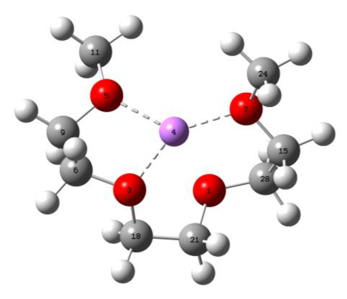
| S/N | Bond Length (Å) | O-Li-O Angle (o) | O-C-C-O Angle (o) |
|---|---|---|---|
| 1 | 5-4 (1.95226) | 5-4-3 (85.81815) | 5-9-6-3 (−47.59083) |
| 2 | 3-4 (1.99950) | 3-4-2 (129.63429) | 3-18-21-1 (−58.34169) |
| 3 | 2-4 (1.95226) | 5-4-2 (135.18919) | 1-28-15-2 (−47.59071) |
Disclaimer/Publisher’s Note: The statements, opinions and data contained in all publications are solely those of the individual author(s) and contributor(s) and not of MDPI and/or the editor(s). MDPI and/or the editor(s) disclaim responsibility for any injury to people or property resulting from any ideas, methods, instructions or products referred to in the content. |
© 2023 by the authors. Licensee MDPI, Basel, Switzerland. This article is an open access article distributed under the terms and conditions of the Creative Commons Attribution (CC BY) license (https://creativecommons.org/licenses/by/4.0/).
Share and Cite
Al-Qatatsheh, A.; Capricho, J.C.; Raiteri, P.; Juodkazis, S.; Salim, N.; Hameed, N. Crosslinking Rapidly Cured Epoxy Resin Thermosets: Experimental and Computational Modeling and Simulation Study. Polymers 2023, 15, 1325. https://doi.org/10.3390/polym15051325
Al-Qatatsheh A, Capricho JC, Raiteri P, Juodkazis S, Salim N, Hameed N. Crosslinking Rapidly Cured Epoxy Resin Thermosets: Experimental and Computational Modeling and Simulation Study. Polymers. 2023; 15(5):1325. https://doi.org/10.3390/polym15051325
Chicago/Turabian StyleAl-Qatatsheh, Ahmed, Jaworski C. Capricho, Paolo Raiteri, Saulius Juodkazis, Nisa Salim, and Nishar Hameed. 2023. "Crosslinking Rapidly Cured Epoxy Resin Thermosets: Experimental and Computational Modeling and Simulation Study" Polymers 15, no. 5: 1325. https://doi.org/10.3390/polym15051325