Article

Characterization of Polyisobutylene Succinic Anhydride (PIBSA) and Its PIBSI Products from the Reaction of PIBSA with Hexamethylene Diamine

Department of Chemistry, Institute for Polymer Research, Waterloo Institute for Nanotechnology, University of Waterloo, 200 University Avenue West, Waterloo, ON N2L 3G1, Canada
*
Author to whom correspondence should be addressed.
Polymers 2023, 15(10), 2350; https://doi.org/10.3390/polym15102350
Submission received: 15 March 2023 / Revised: 12 May 2023 / Accepted: 13 May 2023 / Published: 17 May 2023
(This article belongs to the Special Issue Characterization and Application of Block Copolymers)

Abstract

:
The nature of the end-groups of a PIBSA sample, namely a polyisobutylene (PIB) sample, where each chain is supposedly terminated at one end with a single succinic anhydride group, was characterized through a combination of pyrene excimer fluorescence (PEF), gel permeation chromatography, and simulations. The PIBSA sample was reacted with different molar ratios of hexamethylene diamine to generate PIBSI molecules with succinimide (SI) groups in the corresponding reaction mixtures. The molecular weight distribution (MWD) of the different reaction mixtures was determined by fitting the gel permeation chromatography traces with sums of Gaussians. Comparison of the experimental MWD of the reaction mixtures with those simulated by assuming that the reaction between succinic anhydride and amine occurs through stochastic encounters led to the conclusion that 36 wt% of the PIBSA sample constituted unmaleated PIB chains. Based on this analysis, the PIBSA sample was found to be constituted of 0.50, 0.38, and 0.12 molar fractions of PIB chains that were singly maleated, unmaleated, and doubly maleated, respectively.

Graphical Abstract

1. Introduction

Living polymerization techniques have enabled the preparation of monodisperse polymers that can be modified at one chain end with specific functionalities [1,2,3,4,5] allowing their incorporation into much larger, well-defined macromolecular architectures through a grafting onto scheme [6,7,8]. Such reaction schemes enable the synthesis of highly branched macromolecules with controlled architectures, such as arborescent or dendritic polymers [9,10,11,12,13,14] or polymeric bottle brushes [15,16,17]. The click reaction between an end-modified polymer (EMP) and the appropriate substrate requires that all linear chains be end-modified with a single functionality [1,2,3,4,5,6,7,8,9,10,11,12,13,14,15,16,17,18]. While such conditions can be routinely achieved in a research laboratory, they can be more challenging in industry settings, where side reactions can result in incomplete end-modification and/or incorporation of more than one functionality per chain. Since control over the structural integrity of the final macromolecule depends on the chemical purity of the EMP to be grafted onto the substrate, defects in the EMP must be carefully identified so that they can be accounted for during the grafting onto reaction, particularly when the pure EMP cannot be easily isolated for use in a multistep industrial process.
Unfortunately, the characterization of the functionality of EMPs prepared through an industrial process is often challenging, as highlighted in a recent publication [19]. First, the end groups of a linear chain are present in low abundance, complicating their detection. Second, techniques based on FTIR, UV-Vis, or NMR spectroscopy might yield the average content of a given functionality per unit mass of the EMP but cannot readily assess the absence of functionalization or the single or multiple modifications of a chain end [20]. Third, while relating the number of chain ends to the degree of functionality of an EMP could provide some information about the nature of the modification (absent, single, or multiple), it would require the determination of the number average molecular weight (Mn) of the polymer [20]. Unfortunately, gel permeation chromatography (GPC) is ill-suited to determine the absolute Mn for shorter polymers that yield little signal with a light scattering or viscosity detector and for which standards with a narrow molecular weight distribution (MWD) might not be readily available to calibrate the instrument [21]. Similarly, the determination of Mn by mass spectrometry (MS) is more challenging for polydisperse and apolar polymers [22].
These complications affect the characterization of numerous EMPs prepared industrially, including that of polyisobutylene terminated at one end with succinic anhydride (PIBSA). PIBSA can be obtained through the modification of PIB with maleic anhydride via an Alder-ene reaction [23,24]. PIBSA is an important building block for the synthesis of ashless PIBSI dispersants produced by reacting the terminal succinic anhydrides (SA) of two PIBSA molecules with the two terminal primary amines of a linear polyamine-like tetraethylene pentamine (TEPA) or pentaethylene hexamine (PEHA) [25,26,27]. This reaction produces a PIBSI dispersant by generating two succinimides (SI) connecting two PIB chains to the polyamine core (Scheme 1). PIBSI dispersants are added to engine oil to stabilize the polar particles generated in the oil during the normal operation of the engine, which would otherwise agglomerate and lead to oil thickening [25]. The polar polyamine core of a PIBSI dispersant adheres to the polar surface of insoluble particulates in the oil, while the large apolar PIB segments prevent further aggregation, mainly through steric stabilization [27,28].
As discussed in a recent publication [19], the importance of PIBSI dispersants as oil additives requires that their synthesis be carefully controlled through the use of well-characterized PIBSA blocks. Unfortunately, most techniques typically available in polymer science to characterize macromolecules are ineffective in characterizing the functionality of many EMPs, such as PIBSA. While a combination of pyrene excimer fluorescence, UV-Vis absorption, and 1H NMR analysis can provide the SA content (λSA) and molar fraction (fdoubly) of doubly maleated PIBSA chains (PIBSA2) of a PIBSA sample, which had been determined in an earlier study [19] to equal 0.418 mmol/g and 0.19, respectively, the weight fraction (wPIB) of unmaleated PIB chains remains unknown.
To address this issue, a general methodology is proposed in the present study to determine the weight fraction of unmodified polymers in an EMP sample by using GPC analysis to monitor the reactants and products for a reaction between an EMP sample and a bifunctional linker selected to react effectively with the end groups of the EMP. By taking advantage of the ability of GPC to separate polymer chains according to their size [29,30], GPC analysis of reaction mixtures obtained with different molar equivalents (meq) of EMPs and bifunctional linkers can uncover the amount of unmodified polymer that does not partake in the coupling reaction by taking advantage of the size difference between the doubly and singly appended linkers. The detection of unreacted EMPs in a coupling reaction involving two meq of EMPs and one meq of a bifunctional linker, which should result in the complete consumption of the EMP, is a clear indication that some unmodified polymer is present in the EMP sample, whose weight fraction can be quantified through GPC analysis.
As a case in point, this methodology was applied to a series of reactions referred to as PIBSA–H(X) between a PIBSA sample and a bifunctional linker, namely hexamethylene diamine (HMDA), with different amine-to-SA (X = NAm/NSA) ratios ranging from 0.19 to 1.51. The constituents of the reaction mixtures and their relative contents were characterized by gel permeation chromatography (GPC) analysis, which indicated that a constant amount of PIBSA reactant was unable to react for all amine-to-SA ratios. The unreactive PIBSA species was most likely unmaleated PIB that was unable to participate in the succinimide formation. Careful analysis of the GPC data combined with simulations used to predict the composition of the reaction mixtures led to a highly detailed description of the types of end groups found in the PIBSA sample, with 50, 38, and 12 mol% of the PIB chains being singly maleated, unmaleated, and doubly maleated, respectively. Such detailed end-group analysis of an EMP is required to predict the products of its reaction with a given substrate, and while it was applied to PIBSA as a specific example, the proposed methodology can be extended to any EMP and should thus be of interest to scientists interested in generating complex macromolecular architectures involving reactions with EMPs.

2. Materials and Methods

Chemicals. Xylene (98.5%, Caledon Laboratory Chemicals), tetrahydrofuran (THF, 99%, Sigma-Aldrich, St. Louis, MO, USA or distilled in glass, 99.9%, Fisher Chemical, Hampton, NH, USA), acetone (HPLC grade, Sigma-Aldrich), and hexamethylene diamine (HMDA, 98%, Sigma-Aldrich) were used without further purification. The PIBSA sample was supplied by Afton Chemical.
Fourier-transform infrared (FTIR). A Bruker Tensor 27 FTIR spectrometer was used to obtain the FTIR spectra of the polymer samples. Polymer films were prepared to acquire the FTIR spectra by depositing solutions of the polymer samples in CHCl3 onto a NaCl FTIR cell and evaporating the solvent under N2. The absorbance was then measured from 1000 to 2000 cm−1 and kept around 1.0 to optimize the signal-to-noise ratio.
Gel permeation chromatography (GPC). GPC analysis was conducted with a Viscotek GPC max VE 2001 instrument equipped with two PolyAnalytik columns (PolyAnalytik styrene-divinylbenzene SupeResTM PAS-101 and PAS-103 with exclusion limits of 1.5 × 10³ and 7 × 10⁴ Da, respectively, 8 mm × 30 cm) and a triple-detector array, which included a differential refractive index (DRI), viscosity, and static light scattering detector. THF was used as the solvent. The polymer samples were dissolved in the THF from the GPC reservoir to prepare 1 mg/mL polymer solutions. The polymer solutions were filtered through 0.22 μm PTFE filters before injection.
Fitting the GPC traces with sums of Gaussians: Since sums of Gaussians were used to fit GPC traces [31,32], the DRI traces were baseline corrected and could be fitted with sums of Gaussians as a function of the variable x, which was either the elution volume (Vel) or the degree of polymerization (Xn). The analysis was conducted with the program xgauss written in-house, where x equals mono, bi, tri, tetra, penta, or hexa to fit the DRI traces with a sum of 1–6 Gaussians according to Equation (1), respectively. The sum of Gaussians analysis enabled the mathematical parametrization of the experimental GPC traces, which provided a means to describe them with a small number of parameters. This sum of Gaussians analysis yielded the scaling factor A and the parameters ai, μi, and σi, representing the normalized pre-Gaussian factor, the average, and the standard deviation of the ith Gaussian used to fit the GPC trace. The xgaussSNP program series (where x = mono, bi, and tri) was used to fit a DRI trace with Equation (2), divided into two sums of Gaussians. The parameters ai, μi, and σi used in the first sum had been pre-determined from the xgauss analysis of a DRI trace and were fixed in the analysis with xgaussSNP. The parameters aj, μj, and σj used in the second sum of Gaussians were optimized in the analysis, along with the scaling factors A and B.
D R I ( x ) = A × i = 1 n a i σ i 2 π exp x μ i 2 σ i 2
D R I ( x ) = A × i = 1 n a i σ i 2 π exp x μ i 2 σ i 2 + B × j = 1 m a j σ j 2 π exp x μ j 2 σ j 2
In Equations (1) and (2), all pre-Gaussian and scaling factors were forced to remain positive in the analysis. All floating parameters were optimized according to the Levenberg–Marquardt algorithm for both the xgauss and xgaussSNP fitting programs [33].
Simulating the composition of a reaction mixture between PIBSA and HMDA. The programs reaction3 and reaction4 were created to simulate the molar fractions of the PIBSA reactants and PIBSI products obtained for a coupling reaction between a given amount of PIBSA and HMDA. The parameters to be input into the programs were the number of molecules to be simulated, the molar fraction fdoubly of doubly maleated PIB chains in the PIBSA sample, and the ratio NAm/NSA of the number of amines over the number of succinic anhydrides used for a given coupling reaction. These parameters were then employed to create a list of molecules comprised singly maleated PIBSA1, doubly maleated PIBSA2, and diamine species, with the ratio NPIBSA2/(NPIBSA1 + NPIBSA2) of the number of PIBSA2 molecules over the total number of PIBSA molecules given by fdoubly and the ratio NAm/(NPIBSA1 + 2 × NPIBSA2) being equal to the NAm/NSA ratio. Each molecule in the reaction mixture was defined by its number of PIB chains (nPIB), succinic anhydrides (nSA), and amines (nAm). For instance, a PIBSA2 molecule would be referred to as nPIB = 1, nSA = 2, and nAm = 0. Two molecules defined by the parameters nPIB, nSA, and nAm, namely mol1(nPIB,1, nSA,1, nAm,1) and mol2(nPIB,2, nSA,2, nAm,2) in the list, were then selected at random from the reaction mixture. If nAm ≥ 1 for one molecule and nSA ≥ 1 for the other molecule, the two were combined to form a new molecule mol3(nPIB,3, nSA,3, nAm,3) with nPIB,3 = nPIB,1 + nPIB,2, nSA,3 = nSA,1 + nSA,2 − 1, and nAm,3 = nAm,1 + nAm,2 − 1. The new molecule mol3 was added to the reaction mixture, and mol1 and mol2 were removed before repeating this process until all available amines and/or succinic groups were consumed, i.e., when either NSA = 0 or NAm = 0 in the reaction mixture.
Two programs were implemented based on this concept. The program reaction3 allowed for the coupling of any amine and PIBSA molecule with no limit to the oligomerization of PIBSA molecules through the PIBSA2 species into tri-, tetra-, penta-PIBSIs, etc. The reaction4 program limited the coupling products to contain a maximum of 2 PIBs (nPIB ≤ 2), assuming that steric hindrance prevented oligomerization into higher-order PIBSIs, essentially limiting the PIBSI products to m- and b-PIBSI species. The programs output the number of m-, b-, tri-, tetra-, penta-, hexa-, hepta-, octa-, and nona-PIBSIs resulting from the coupling reaction of PIBSA and diamines, which could be used to determine the molar fraction of each PIBSI species in the reaction mixture.
Calibration of the GPC instrument with polydisperse PIB standards. The 2nd order polynomial [Ln(M) = b0 + b1Vel + b2Vel2] obtained as Equation (S13) in Supplementary Material was used as the Ln(M)-vs-Vel calibration curve, which was established using the baseline-corrected DRI traces of a set of 3 PIB standards with a broad MWD purchased from Polymer Source. The probability P(M) of having a molar mass M for a PIBSA–H(X) mixture was obtained by applying Equation (3), where the function DRI(Vel) corresponds to the GPC trace obtained for the PIBSA–H(X) mixture with the DRI detector. The derivation of P(M) is provided in Supplementary Material, where it is given as Equation (S9) [34].
P ( M ) = 1 0 D R I ( V e l ) exp ( i = 0 n b i V e l i ) d V e l × D R I ( V e l ) exp 2 × i = 0 n b i V e l i × i = 1 n i b i V e l i 1
Synthesis of PIBSA–HMDA samples. The PIBSA sample received from Afton Chemical had an fdoubly of 0.19, as previously determined [19], and was reacted with varying amounts of HMDA to form m-PIBSI, b-PIBSI, and possibly other higher-order PIBSI products enabled by the presence of PIBSA2, according to Scheme 2.
The NAm/NSA ratio was varied from 0.19 to 1.51 in 0.19 increments to study how this ratio would affect the proportion of reactants and products generated during the coupling reactions. The proportion of PIBSA was expected to decrease as the NAm/NSA ratio increased from 0.19 to 1.0, as more amine is provided for coupling PIBSA into b-PIBSI and higher-order PIBSI dispersants [33]. The proportion of m-PIBSI should increase when the NAm/NSA ratio increases from 1.0 to 1.51, as PIBSA molecules are ‘capped’ by the excess amines, resulting in more m-PIBSIs bearing a free amine. The reaction with an NAm/NSA ratio of 0.38 is explained in more detail as an example.
PIBSA (6.3 g) was dissolved in 8 mL of THF and precipitated with 200 mL acetone to remove low molecular weight impurities along with the low molecular weight fraction of the MWD. The mixture was then decanted, and PIBSA was dried overnight under vacuum at 70 °C. PIBSA (0.93 g) was dissolved in 20 mL of hot xylene, and the hot PIBSA solution was added to a 100 mL round bottom flask (RBF), which was connected to a Dean-Stark condenser and kept under nitrogen. The solution was refluxed overnight in an oil bath at 175 °C to dehydrate the partially hydrated PIBSA sample and regenerate succinic anhydride from the succinic acid groups. An aliquot was taken the next day to acquire an FTIR spectrum (see Spectrum A in Figure 1) to confirm dehydration of PIBSA via the disappearance of the absorbance peak at 1710 cm−1, characteristic of succinic acid carbonyl.
The succinic anhydride content (λSA) of 0.418 mmol/g for the PIBSA sample was determined from a combination of pyrene excimer fluorescence, 1H NMR, and UV-Vis spectroscopy, as described earlier [19]. HMDA (8.7 mg, 0.075 mmol) was dissolved in 20 mL of hot xylene and added to the reaction vessel containing the dehydrated PIBSA sample (0.39 mmol SA) in xylene to react overnight at reflux. The next morning, an aliquot was taken from the reaction mixture to acquire an FTIR spectrum, shown as Spectrum B in Figure 1. The FTIR spectrum confirmed the completion of the reaction with the presence of the succinimide absorption band at 1705 cm−1. The spectrum also lacked strong amide absorption at 1650 cm−1, which would have indicated incomplete cyclization of the succinamic acids into succinimides, as observed in the labeling of PIBSA with 1-pyrenemethylamine in previous work [19].
Since the NAm/NSA ratio was below 1, the final product would include both succinimide and succinic anhydride groups, as not enough amines could react with the succinic anhydride groups, resulting in the succinimide and succinic anhydride absorption bands in Spectrum B in Figure 1. After the reaction was complete, the reaction mixture was condensed and dissolved in THF before being transferred to a 20 mL vial. The THF was evaporated under a flow of nitrogen before the polymer product was dried to completion in a vacuum oven at 70 °C overnight to yield the PIBSA–H(0.38) reaction mixture. After being removed from the vacuum oven, the PIBSA–H(0.38) sample was dissolved in THF for GPC analysis. PIBSA–H(X) samples were prepared for NAm/NSA ratios ranging from X = 0.19 to 1.51 in 0.19 increments, and the different samples were characterized by FTIR and GPC analyses in the same manner.

3. Results and Discussion

As illustrated in an earlier publication [35], the reaction of PIBSA with HMDA generates b-PIBSI and higher-order PIBSI products, which shift the MWD of the reaction mixture to higher molecular weights. As a result, the GPC traces acquired in that study showed a shift to lower elution volumes. This observation was taken advantage of in the present study to conduct a more detailed analysis of the GPC traces based on sums of Gaussians to determine the weight fraction (wPLM) of PIBSA-like molecules (PLM), being either a PIBSA reactant, a m-PIBSI product, or an unmaleated PIB chain, present in a PIBSA–H(X) reaction mixture. The chemical composition of the PIBSA–H(X) reaction mixtures was first characterized in terms of their content of SA and succinimide functionalities, which were determined from the analysis of their FTIR spectra.

3.1. Analysis of the Fourier-Transform Infrared (FTIR) Spectra

FTIR spectroscopy was used to monitor the coupling of PIBSA with HMDA at different NAm/NSA ratios. The content of SA and succinimide groups was monitored by the intensity of their absorption bands at 1785 and 1705 cm−1, respectively [19,33,34]. The FTIR spectra of the PIBSA–H(X) coupling products, where X is the NAm/NSA ratio used in a given coupling reaction, are shown in Figure S1 in the Supplementary Material. The FTIR spectra in Figure S1 shared most of the same features, notably the characteristic PIB peaks from the methyl swinging motions at 1365 and 1390 cm−1 and methylene bending and scissoring peaks at 1225 and 1465 cm−1, respectively [19,33,36]. The PIBSA–H(1.51) sample had a small amide peak at 1650 cm−1, which was not as prevalent in the other samples with lower NAm/NSA ratios, possibly due to its increased amine content.
The Abs(1785 cm1)/Abs(1390 cm1) and Abs(1705 cm1)/Abs(1390 cm1) ratios, taken as measures of the SA and succinimide contents in the reaction mixture, respectively, were plotted as a function of the NAm/NSA ratio in Figure 2 to monitor the composition of the reaction mixture as more hexamethylene diamine was added to the PIBSA sample. The Abs(1785 cm1)/Abs(1390 cm1) ratio decreased with increasing NAm/NSA ratio, as expected, approaching zero for an NAm/NSA ratio equal to 1 and remaining close to zero for NAm/NSA ratios greater than 1. The non-zero values of the Abs(1785 cm1)/Abs(1390 cm1) ratio for NAm/NSA ratios greater than 1 could be due to the weak secondary absorption band of the succinimide at 1775 cm1, which increased in intensity with increasing NAm/NSA ratios (see Figure S1). The Abs(1705 cm1)/Abs(1390 cm1) ratio was weak for the PIBSA–H(0.19) product as little succinimide was formed, and it increased with an increasing NAm/NSA ratio, as expected. In summary, the FTIR spectra showed that the coupling reactions between PIBSA and HMDA were efficient and that the IR absorbance of the succinimide and succinic anhydride carbonyls followed the expected trends.

3.2. Gel Permeation Chromatography (GPC) Analysis

The program tetragauss was used to fit the GPC trace of the PIBSA sample with a sum of four Gaussians, according to Equation (1), and the parameters used in the fit were fixed in the analysis of the GPC traces obtained for the PIBSA–H(X) mixtures with the program xgaussSNP, according to Equation (2). The xgaussSNP programs enabled the isolation of the PLM contribution in the PIBSA–H(X) mixtures. The fits of the GPC traces started with one Gaussian whose parameters were allowed to float, adding one Gaussian with floating parameters at a time to the sum, and comparing the squared difference between the experimental and calculated GPC profiles for each fit until the difference showed little variation with an increasing number of Gaussians. This procedure resulted in good fits for the GPC traces, as illustrated in Figure 3 for the PIBSA sample and Figure 4 for all of the PIBSA–H(X) reaction mixtures.
The DRI trace in Figure 4A reached its maximum at an elution volume of 16.7 mL, similar to the DRI trace of PIBSA in Figure 3. However, as more HMDA was added to the reaction mixtures, the peak maximum of the DRI traces in Figure 4B–E shifted to a lower elution volume of 15.6 mL while retaining a shoulder on the low molecular weight side corresponding to the contribution from PLM, which decreased with an increasing NAm/NSA ratio. As the NAm/NSA ratio increased past unity, the maximum of the DRI traces in Figure 4F–H remained at 15.6 mL, but the contribution from PLM increased, appearing as a shoulder on the low molecular weight side of the distribution. Finally, one advantage of the fits with sums of Gaussians was the elimination of the small peaks, which appeared at the low molecular weight end of the GPC traces in Figure 3 and Figure 4 and could have been due to residual traces of solvent and/or HMDA remaining in the samples.
Since the fits of the DRI traces with a sum of Gaussians in Figure 4 gave a good representation of the PIBSA/PIBSI species without the solvent peaks in the PIBSA–H(X) mixtures, they were used to represent the experimentally obtained DRI traces and are referred to as the experimental* DRI traces from this point on. Examples of the traces obtained by fitting the PIBSA–H(0.75) DRI trace with trigaussSNP and the comparison of the fits with sums of Gaussians of the PIBSA–H(X) samples having NAm/NSA ratios ranging from 0.19 to 0.94 and from 0.94 to 1.51 are shown in Figure 5A–C, respectively.
In the trigaussSNP analyses, PIBSA and m-PIBSI were assumed to share the same MWD, and both molecules are referred to as PIBSA-like molecules (PLM). The ability to decompose the MWD of the reaction products into PLM and non-PIBSA-like molecules (non-PLM) through the analysis of the DRI traces with sums of Gaussians enabled the determination of the weight fraction (wPLM) of PLM in the reaction mixture from the ratio A/(A + B), where A and B are the pre-factors used in Equation (2), since the DRI signal is proportional to the mass concentration of the polymer passing through the detector. A plot of wPLM as a function of the NAm/NSA ratio is presented in Figure 5D. For NAm/NSA ratios lower than unity, wPLM first decreased with increasing NAm/NSA, as b-PIBSI and higher-order PIBSI oligomers were produced in the reaction, until the NAm/NSA ratio reached unity and wPLM passed through a minimum. As the NAm/NSA ratio increased past unity, more m-PIBSI was generated, and wPLM increased slightly with the increasing NAm/NSA ratio. The most noticeable feature of Figure 5D was that the wPLM did not reach zero at a NAm/NSA ratio of unity. This observation suggested that a significant number of PIBSA molecules, probably unmaleated PIB chains, did not react with HMDA. Taking the lowest wPLM value obtained in Figure 5D as the weight fraction of unmaleated PIB (wPIB) would suggest that 37 wt% of unmaleated PIB chains are present in the PIBSA sample.
Comparison of the traces in Figure 5B,C revealed some interesting trends for the PIBSA–H(X) products. The MWD shifted to lower elution volumes when the NAm/NSA ratio increased from 0.19 to 0.94 in Figure 5B, as would be expected if more diamines were added to favor the coupling with PIBSA molecules into b-PIBSI and higher-order PIBSI products. The high molecular weight region of the DRI traces in Figure 5C appeared to have roughly the same front in the low Vel region and peak maximum, inferring that the same higher-order PIBSI products were generated at NAm/NSA ratios ≥ 1. To further examine this conclusion, the contribution of the non-PLM in the experimental* DRI traces was overlaid in Figure 6A,B for NAm/NSA ratios between 0.19 and 0.94 and between 0.94 and 1.51, respectively.
The traces in Figure 6B showed that the non-PLM in the PIBSA–H(X) mixtures had a similar MWD for all NAm/NSA ratios ≥ 0.94, inferring that the coupling reaction must be producing the same higher-order PIBSI products regardless of the NAm/NSA ratio. The non-PLM contribution in the DRI traces for the NAm/NSA ratios of 0.38 and 0.56 shown in Figure 6A had a shoulder in the low MW region of the MWDs, where PIBSA is expected to elute. This observation would imply that the fraction of the PLM in these samples was underestimated, even more so for the PIBSA–H(0.38) sample, which had a larger shoulder.
The main conclusion from the analysis of the DRI traces in Figure 6 is that they could be decomposed into just two contributions: one contribution for PLMs, referring to PIBSA, m-PIBSI, or non-maleated PIB chains, which would be indistinguishable; and another contribution for the same higher-order PIBSI product. Since the shape of the DRI traces in Figure 6, which describes the MWD of the higher-order PIBSI products, did not seem to change much with the NAm/NSA ratio, it suggests that the same higher-order PIBSI product was being generated and that this product was b-PIBSI. To elaborate further on this proposal, the experimental* DRI traces were fitted with a linear regression, assuming that they were the sum of two contributions, one for PLMs and the other for the non-PLM portion of the PIBSA–H(0.94) sample in Figure 6, taken as a representative MWD of the non-PLM produced in the PIBSA–H(X) reactions. The wPLM fractions obtained by fitting the experimental* DRI traces of the PIBSA–H(X) mixtures with a sum of Gaussian fit or a linear regression were compared in Figure 5D. When plotted against NAm/NSA in Figure 5D, similar wPLM values were obtained for the PIBSA–H(X) reaction mixtures, regardless of the fitting method.
The DRI traces obtained by applying a linear regression with one contribution for PLMs and another for non-PLMs were compared to the experimental* DRI traces in Figure 7. While there were some slight deviations from the experimental* DRI traces near the peak maxima, as in Figure 7B,H, the regressions gave a fairly good representation of the experimental* DRI traces of each PIBSA–H(X) sample. The good agreement between the experimental* DRI traces and those synthesized using two set contributions supports the earlier suggestion that the coupling reaction between PIBSA and HMDA might be producing the same higher-order b-PIBSI product regardless of the NAm/NSA ratio applied. The good agreement between the results obtained from the fit of the DRI traces with a linear regression or the xgaussSNP programs suggests that the proposed analysis could successfully characterize the products of the PIBSA–H(X) reactions based only on a GPC instrument with a DRI detector and the Gaussian fitting programs developed in house.
Unfortunately, the experimental validation of the trivial proposal that the MWD shown in Figure 7 can be decomposed into two contributions of PLM and non-PLM is challenging for the following reasons. First, three different polymer types, namely PIB, PIBSA composed of PIBSA1 and PIBSA2, and mPIBSI, constitute the PLM and cannot be isolated or individually characterized due to their similar chemical compositions. Second, the MWD of the b-PIBSI and higher-order PIBSI species constituting the non-PLM shows a significant overlap with the MWD of the PLM in Figure 6, indicating that both PLM and non-PLM elute together in the GPC instrument. Third, a complete compositional analysis of all the different species present in a PIBSA–H(X) reaction mixture separated according to their size by GPC cannot be accomplished because GPC does not have the resolution capability to distinguish at each elution volume between so many different polymeric species that share a similar chemical composition consisting mostly of PIB and differentiated by only one or two SA or SI groups.
Instead, simulation programs were implemented to predict the molar fractions of different reaction products that could be made in a given PIBSA–H(X) reaction. In turn, these molar fractions could be used in combination with the DRI traces corresponding to the PLM and non-PLM species in Figure 6 to generate theoretical DRI traces that could be compared with the experimental* DRI traces shown in Figure 7. A reasonable agreement between the simulated and experimental* DRI traces would then be taken as validation of the composition of the different components present in a given PIBSA–H(X) reaction mixture that would have been predicted by the simulations. The implementation of these simulations is described in the following section.

3.3. Simulations to Predict the Composition of a PIBSA–H(X) Reaction Mixture

To predict the composition of the PIBSA–H(X) mixtures in terms of PLM and non-PLM contributions, the coupling programs reaction3 and reaction4 were created to simulate the products of a coupling reaction between PIBSA and HMDA based on the known molar fraction (fdoubly) of doubly modified PIBSA2 in the PIBSA sample and the NAm/NSA ratio used in the reaction. Since the non-PLM fraction of the PIBSA–H(X) mixtures shared a common MWD, in Figure 6, the proposal was made that the PIBSA–H(X) coupling reactions might yield the same higher-order PIBSI product regardless of the NAm/NSA ratio. The similarity of the non-PLM products suggested that only b-PIBSI dimers were formed, possibly due to the short span of HMDA giving rise to steric hindrance when trying to couple two PIBSAs to the same PIBSA2 molecule. If steric hindrance were preventing the formation of tri-PIBSA or higher-order PIBSI products in the PIBSA–H(X) coupling reactions, only b-PIBSI dimers would form, which would result in the same non-PLM fraction in all the DRI profiles regardless of the NAm/NSA ratio, as concluded from the GPC analysis shown in Figure 6B. While this would eliminate the formation of higher-order structures such as tri-PIBSI, the fdoubly value for the PIBSA sample of interest would still need to be taken into consideration in simulations to account for the extra succinic anhydride in PIBSA2, which would consume the amines of HMDA, but not append an additional PIBSA if the neighboring succinic group of a PIBSA2 molecule had already been coupled to another PIBSA to form b-PIBSI.
To further study these possibilities, two simulation programs were implemented. The program reaction3 was created to predict the molar fractions of m-PIBSI, b-PIBSI, and higher-order PIBSIs expected if the coupling between PIBSA and HMDA was not sterically hindered. Similarly, the reaction4 program was created to predict the molar fractions of PLMs and b-PIBSI products expected from the coupling of PIBSA and HMDA, while assuming that a PIBSA2 molecule could react with two diamines but only one other PIBSA molecule due to steric hindrance, which would limit the PIBSI products to only m-PIBSI and b-PIBSI.
A fdoubly value of 0.19, determined earlier for the PIBSA sample [19], was used in the reaction3 and reaction4 programs. Each of the reaction3 and reaction4 programs was carried out with 1000 PIBSA molecules and averaged over 100 simulations using NAm/NSA ratios of 0.19, 0.38, 0.56, 0.75, 0.94, 1.13, 1.32, 1.51, 1.75, and 2.00. For each coupling reaction, the number of product molecules with different numbers of PIB segments (nPIB) and SA (nSA) and Am (nAm) groups was compiled, and the resulting numbers of PIBSA and PIBSI species are listed in Tables S5 and S6 in the Supplementary Material. The numbers of PIBSA and PIBSI molecules were used to calculate the molar fractions fPIBSA, fPIB1SI, fPIB2SI, fPIB3SI… of the different species PIBSA, m-PIBSI, b-PIBSI, tri-PIBSI…, and these molar fractions were then employed to calculate w P L M s i m , as shown in Equation (4).
w P L M s i m = f PIBSA + f PIB 1 SI f PIBSA + f PIB 1 SI + i = 2 n i × f PIB i SI
The w P L M s i m fractions predicted from both simulation programs were plotted as a function of the NAm/NSA ratio in Figure 8A. w P L M s i m decreased steeply as the NAm/NSA ratio increased from 0.19 to 0.94, before increasing gently with increasing NAm/NSA ratios from 0.94 to 2.0. Both simulations yielded similar w P L M s i m fractions for all NAm/NSA ratios. The V-shaped w P L M s i m -vs-NAm/NSA plot obtained with the simulations closely mirrored the experimental wPLM obtained by GPC analysis with sums of Gaussians or linear regression in Figure 5D. The only noticeable difference was that the plot obtained by simulations yielded a zero- w P L M s i m fraction for the PIBSA–H(1) reaction mixture, whereas the experimental wPLM fraction was significantly larger than zero. The only possible explanation for this discrepancy was that the PIBSA sample contained unmaleated PIB chains that did not participate in the coupling reaction with HDMA. To account for the presence of unmaleated PIB in the PIBSA sample, the weight fraction of unmaleated PIB (wPIB) could be simply estimated from Equation (5), whose derivation is provided in the Supplementary Material.
w P I B = w P L M w P L M s i m 1 w P L M s i m
A plot of wPIB as a function of NAm/NSA is shown in Figure 8B. Excepting the wPIB value obtained for an NAm/NSA ratio of 0.19, which was probably an outlier, the wPIB values shown in Figure 8B remained fairly constant with the NAm/NSA ratio and took an average wPIB value of 0.36 (±0.08) when calculated with either reaction3 or reaction4. This analysis suggested that 36 wt% of the PIBSA sample was unmaleated PIB, in good agreement with the 37 wt% prediction, which was made earlier based on the trends shown in Figure 5D. The same weight fraction wPIB of 0.36 was then used to calculate w P L M c a l equal to w P L M s i m + wPIB × (1 − w P L M s i m ) based on Equation (5), which was compared in Figure 8C to the experimental wPLM fractions obtained from the regression fits in Figure 5A for the PIBSA–H(X) mixtures. Without including wPIB, w P L M s i m showed a similar trend in Figure 8A to that of wPLM obtained experimentally by GPC analysis, but w P L M s i m was shifted to lower values. Upon including wPIB equal to 0.36 in the calculation of w P L M c a l , good agreement was obtained between the calculated w P L M c a l and experimental wPLM weight fractions in Figure 8C.

3.4. Predicted MWD of b-PIBSI Supports That b-PIBSI Is the Only Higher-Order PIBSI Product

A procedure was implemented as in the Supplementary Material to establish a calibration curve (see Equation (S13)) for the GPC instrument based on PIB standards having a broad MWD. The calibration curve was applied to the DRI trace obtained for the PIBSA sample to obtain its MWD, given by P(M) in Equation (3), also referred to as P1(M) for the PIBSA unimer. P1(M) was plotted as a function of M in Figure 9A. Equations (S10) and (S11) could be applied to determine the number (Mn) and weight (Mw) average molecular weight of PIBSA, which were found to equal 1.3 and 2.6 kg/mol, respectively. The Mn value of 1.3 kg/mol agreed with the location of the DRI trace of PIBSA with respect to the two PIB standards in Figure 9A, since it was much closer to the DRI trace of the PIB standard with an Mn equal to 1.0 kg/mol compared to that of the PIB standard with an Mn of 3.2 kg/mol.
P1(M), shown as a solid trace in Figure 9A, was used to predict the MWD of higher-order PIBSI oligomers using the prod-dis2 coupling program. The program worked by transforming P1(M) into P1(i), where i is the degree of polymerization of a PIBSA molecule having a molecular weight M (i = M/Mo, where Mo is the molar mass of an isobutylene structural unit equal to 56.11 g/mol). The probability Pz(i) of a higher-order (z = 2, 3,…) PIBSI product could then be obtained with Equation (6), where the probability Pz−1(i) represents the MWD of the z − 1 order PIBSI product. For example, coupling the MWD (P1(i)) of PIBSA with itself yields the MWD (P2(i)) of b-PIBSI, coupling the MWDs of (P1(i)) PIBSA and (P2(i)) b-PIBSI yields the MWD (P3(i)) of tri-PIBSI, etc.
P z ( i ) = k = 1 i P 1 ( k ) × P z 1 ( i + 1 k )
Equation (6) was applied to determine all of the functions Pz(M) required for the higher-order PIBSI constructs obtained in the simulations, but only the functions P1(M), P2(M), P3(M), and P4(M) were plotted as a function of M in Figure 9B. The functions shifted to higher molecular weights with increasing z, as would be expected since a higher z indicates a higher order and thus a larger PIBSI product. However, the increase in molecular weight should be considered an apparent increase since PIBSI products of orders higher than 2 have a structure closer to that of a star polymer with a hydrodynamic volume (Vh) that is smaller than that of the linear polymer of an equivalent molecular weight. Since the calibration curve of the GPC instrument is based on linear PIB standards, the molecular weights predicted with Equation (6), which assumes that the coupling between linear PIB molecules results in longer linear PIB chains, would predict larger molecular weights than those found from the GPC analysis based on the calibration curve given in Equation (S13). Consequently, the MWD predicted with Equation (6) for b-PIBSI should be correct since it is a linear polymer, but that for tri-PIBSI and higher-order PIBSI products should be overestimated. Nevertheless, these latter PIBSI products should yield an MWD that is shifted to higher molecular weights compared to that of b-PIBSI, albeit with a smaller shift than predicted in Figure 9B.
In order to assess how the MWD for the higher PIBSI products generated in the PIBSA–H(X) reactions found experimentally in Figure 6B would compare to those predicted from Equation (6), the MWD of the higher-order PIBSI products obtained for the PIBSA–H(0.94) reaction in Figure 6B was compared to the Pz(M) distributions with z equal to 1–4 in Figure 9B. The MWD obtained for the higher-order products in the PIBSA–H(0.94) reaction mixture had been found to be representative of the higher PIBSI products generated in all of the PIBSA–H(X) reactions with X ≥ 0.94 (see Figure 6B). As it turns out, the MWD of the higher-order products found for the PIBSA–H(0.94) reaction appeared to match remarkably well the P2(M) function in Figure 9B, further supporting the notion that b-PIBSI was the highest-order product generated in the PIBSA–H(X) reactions.
Since all lines of investigation support that b-PIBSI is the highest-order product generated in the PIBSA–H(X) reactions, synthetic DRI traces were built for the PIBSA–H(X) reaction mixtures based on the molar fractions fPIB, fPIBSA, fPIB1SI, and fPIB2SI obtained in Table S6 with the simulation program reaction4 and the MWD obtained for PIBSA and the higher-order products in the PIBSA–H(0.94) mixture. The resulting DRI traces were then compared in Figure 10 to the experimental* DRI traces.
The results shown in Figure 10 indicate strong agreement between the experimental* and synthesized DRI traces. Since the synthesized DRI traces were based on the molar fractions obtained with the simulation program reaction4, which assumed that steric hindrance prevented the formation of tri-PIBSI and higher-order PIBSI products, the good agreement between the traces shown in Figure 10 further supports this claim. This good agreement also validates the composition of the PIBSA–H(X) reaction mixtures determined through the simulation programs, as such detailed information about the different PIB species present in the reaction mixture would be difficult to determine experimentally.
The synthesized and experimental* DRI traces shown in Figure 10 were then analyzed using the calibration curve in Equation (S13), which was generated for the GPC instrument, to obtain Mn, Mw, and the polydispersity index (PDI) for the PIBSA–H(X) reaction mixtures. They are plotted as a function of the NAm/NSA ratio in Figure 11. The Mn and Mw values increased when the NAm/NSA ratio increased from 0.19 to 0.94, before decreasing slightly when the NAm/NSA ratio increased from 0.94 to 1.51. These trends mirrored the large decrease in the experimental weight fraction of PLM (wPLM) upon increasing the NAm/NSA ratio from 0.19 to 0.94, before showing a slight increase when the NAm/NSA ratio increased further from 0.94 to 1.51, as seen in Figure 8. Both trends reflected the shift towards the formation of more b-PIBSI products, as the NAm/NSA ratio increased from 0.19 to 0.94 before more m-PIBSI was generated when the NAm/NSA ratio increased from 0.94 to 1.51. In summary, the experimental results seem to agree well with the simulated data, further supporting the conclusion that 36 wt% of unmaleated PIB was present in the PIBSA sample and that steric hindrance prevents the formation of PIBSI products with more than two PIB chains. Taking the fdoubly and wPIB values of 0.19 and 0.36, respectively, the PIBSA chains could be determined to be composed of 50, 38, and 12 mol% of singly maleated, unmaleated, and doubly maleated PIB chains, respectively. Consequently, the proposed methodology that was applied to this PIBSA sample provided a complete characterization of the PIBSA chain ends.

4. Conclusions

PIBSA molecules are an essential component in the preparation of PIBSI dispersants used as engine oil additives. Since the properties of PIBSI dispersants are a result of their chemical architecture, which is itself a direct consequence of the chemical composition of the PIBSA starting material, the characterization of PIBSA samples has been the focus of intense research [8,23,24,37,38,39,40,41,42]. Despite the numerous challenges complicating the characterization of PIBSA samples [19], this study provides a protocol that can be implemented to determine the weight fraction wPIB of unmaleated PIB chains in a PIBSA sample by analyzing the GPC traces obtained with a DRI detector of PIBSA–H(X) reaction mixtures obtained from the reaction between different amounts of PIBSA and HMDA. Furthermore, a theoretical framework was introduced whereby the composition of PIBSI products could be predicted from simulations based on the knowledge of wPIB, fdoubly, and λSA used to characterize the PIBSA sample and the ratio of NAm/NSA, reflecting the amounts of PIBSA and HMDA used in a PIBSA–H(X) reaction.
To the best of our knowledge, this study represents the most extensive investigation reported in the literature aiming to characterize the chemical composition of PIBSA, a key building block in the preparation of PIBSI dispersants used as engine oil additives. It also introduces a general method based on the coupling of two end-modified linear chains that yield the weight fraction of non-modified chains, an important aspect in the characterization of EMPs used in the preparation of large macromolecules with complex architectures [6,7,8,9,10,11,12,13,14,15,16,17].

Supplementary Materials

The following are available online at https://www.mdpi.com/article/10.3390/polym15102350/s1, Figure S1: FTIR spectra for the PIBSI–H(X) samples, Table S1: Mn and Mw values of the PIB standards used for the GPC calibration and determined using the calibration curve from the program cal-2, Table S2: Pre-Gaussian factors, averages, and standard deviations retrieved from the fit of the DRI trace of the PIBSA sample as a function of (Vel) weight tetragauss according to Equation (1), Table S3: Pre-Gaussian factors, averages, and standard deviations retrieved from the fit of the DRI traces of the PIBSA–H(X) samples as a function of (Vel) with xgaussSNP (x = bi, tri) according to Equation (2), Table S4: Pre-Gaussian factors, averages, and standard deviations retrieved from the fit of the simulated MWDs obtained for m-, b-, tri-, tetra-, penta-, hexa-, hepta-, octa-, and nona-PIBSI as a function of (Xn) with xgauss (x = penta, and hexa) according to Equation (1), Table S5: PIBSI products simulated by the reaction3 coupling program, Table S6: PIBSI products simulated by the reaction4 coupling program. Methodology for the GPC calibration curve determination; FTIR spectra; Gaussian fitting parameters; PIBSA coupling products retrieved from simulation programs; determination of wPIB.

Author Contributions

F.F. conducted all the experiments and data analyses and wrote the reaction3 and reaction4 programs and manuscript. J.D. supervised the work, wrote several programs used in the study, and finalized the manuscript for submission. All authors have read and agreed to the published version of the manuscript.

Funding

Funding for this research was provided by Afton Chemical.

Acknowledgments

F.F. and J.D. thank Afton Chemical for generous funding.

Conflicts of Interest

The authors declare no conflict of interest.

References

  1. Lunn, D.J.; Discekici, E.H.; Read de Alaniz, J.; Gutekunst, W.R.; Hawker, C.J. Established and Emerging Strategies for Polymer Chain-End Modification. J. Polym. Sci. A Polym. Chem. 2017, 55, 2903–2914. [Google Scholar] [CrossRef]
  2. Dey, A.; Haldar, U.; De, P. Block Copolymer Synthesis by the Combination of Living Cationic Polymerization and Other Polymerization Methods. Front. Chem. 2021, 9, 644547. [Google Scholar] [CrossRef]
  3. Hilf, S.; Kilbinger, A.F.M. Functional End Groups for Polymers Prepared Using Ring-Opening Metathesis Polymerization. Nat. Chem. 2009, 1, 537–546. [Google Scholar] [CrossRef]
  4. Kim, J.; Jung, H.Y.; Park, M.J. End-Group Chemistry and Junction Chemistry in Polymer Science: Past, Present, and Future. Macromolecules 2020, 53, 746–763. [Google Scholar] [CrossRef]
  5. Zhou, D.; Zhu, L.-W.; Wu, B.-H.; Xu, Z.-K.; Wan, L.-S. End-Functionalized Polymers by Controlled/Living Radical Polymerizations: Synthesis and Applications. Polym. Chem. 2022, 13, 300–358. [Google Scholar] [CrossRef]
  6. Yu, X.; Li, Y.; Dong, X.-H.; Yue, K.; Lin, Z.; Feng, X.; Huang, M.; Zhang, B.-W.; Cheng, S.Z.D. Giant Surfactants Based on Molecular Nanoparticles: Precise Synthesis and Solution Self-Assembly. J. Polym. Sci. B Polym. Phys. 2014, 52, 1309–1325. [Google Scholar] [CrossRef]
  7. Coudane, J.; Nottelet, B.; Mouton, J.; Garric, X.; Van Den Berghe, H. Poly(e-caprolactone)-Based Graft Copolymers: Synthesis Methods and Applications in the Biomedical Field: A Review. Molecules 2022, 27, 7339. [Google Scholar] [CrossRef] [PubMed]
  8. Soares, D.C.F.; Oda, C.M.R.; Monteiro, L.O.F.; Branco de Barros, A.L.; Tebaldi, M.L. Responsive Polymer Conjugates for Drug Delivery Applications: Recent Advances in Bioconjugation Methodologies. J. Drug Target. 2019, 27, 355–366. [Google Scholar] [CrossRef]
  9. Gauthier, M. Arborescent Polymers and Other Dendigraft Polymers: A Journey into Structural Duversity. J. Polym. Sci. A Polym. Chem. 2007, 45, 3803–3810. [Google Scholar] [CrossRef]
  10. Teertstra, S.; Gauthier, M. Dendrigraft Polymers: Macromolecular Engineering on a Mesoscopic Scale. Prog. Polym. Sci. 2004, 29, 277–327. [Google Scholar] [CrossRef]
  11. Tomalia, D.A.; Fréchet, J.M. Discovery of Dendrimers and Dendritic Polymers: A Brief Historical Perspective. J. Polym. Sci. A Polym Chem. 2002, 40, 2719–2728. [Google Scholar] [CrossRef]
  12. Hadjichristidis, N.; Pitsikalis, M.; Pispas, S.; Iatrou, H. Polymers with Complex Architecture by Living Anionic Polymerization. Chem. Rev. 2001, 101, 3747–3792. [Google Scholar] [CrossRef]
  13. Zhang, H.; Zhao, T.; Newland, B.; Liu, W.; Wang, W.; Wang, W. Catechol Functionalized Hyperbranched Polymers as Biomedical Materials. Prog. Polym. Sci. 2018, 78, 47–55. [Google Scholar] [CrossRef]
  14. Blasco, E.; Pinol, M.; Oriol, L. Responsive Linear-Dendritic Block Copolymers. Macromol. Rapid Commun. 2014, 35, 1090–1115. [Google Scholar] [CrossRef]
  15. Lee, H.-I.; Pietrasik, J.; Sheiko, S.S.; Matyjaszewski, K. Stimuli-Responsive Molecular Brushes. Prog. Polym. Sci. 2010, 35, 24–44. [Google Scholar] [CrossRef]
  16. Sheiko, S.S.; Sumerlin, B.S.; Matyjaszewski, K. Cylindrical Molecular Brushes: Synthesis, Characterization, and Properties. Prog. Polym. Sci. 2008, 33, 759–785. [Google Scholar] [CrossRef]
  17. Pelras, T.; Mahon, C.S.; Mullner, M. Synthesis and Applications of Compartmentalized Molecular Polymer Brushes. Angew. Chem. Int. Ed. 2018, 57, 6982–6994. [Google Scholar] [CrossRef] [PubMed]
  18. Chernikova, E.V.; Kudryavtsev, Y.V. RAFT-Based Polymers for Click Reactions. Polymers 2022, 14, 570. [Google Scholar] [CrossRef] [PubMed]
  19. Frasca, F.; Duhamel, J. End Group Analysis of Polyisobutyelene Succinic Anhydride (PIBSA) Carried Out with Pyrene Excimer Fluorescence. Ind. Eng. Chem. Res. 2022, 61, 14747–14759. [Google Scholar] [CrossRef]
  20. Jerome, R.; Henrioulle-Grandville, M.; Boutevin, B.; Robin, J.J. Telechelic Polymers: Synthesis, Characterization and Applications. Prog. Polym. Sci. 1991, 16, 837–906. [Google Scholar] [CrossRef]
  21. Striegel, A.M. There’s Plenty of Gloom at the Bottom: The Many Challenges of Accurate Quantitation in Size-Based Oligomeric Separation. Anal. Bional. Chem. 2013, 405, 8959–8967. [Google Scholar] [CrossRef]
  22. Harrison, J.J.; Mijares, C.M.; Cheng, M.T.; Hudson, J. Negative Ion Electrospray Ionization Mass Spectrum of Polyisobutenylsuccinic anhydride: Implications for Isobutylene Polymerization. Macromolecules 2002, 35, 2494–2500. [Google Scholar] [CrossRef]
  23. Tessier, M.; Maréchal, E. Synthesis of Mono and Difunctional Oligoisobutylenes-III. Modification of α-Chlorooligobutylene by Reaction with Maleic Anhydride. Eur. Polym. J. 1984, 20, 269–280. [Google Scholar] [CrossRef]
  24. Tessier, M.; Maréchal, E. Synthesis of α-phenyl-ω-anhydride oligoisobutylene and α, ω-dianhydride oligoisobutylene. Eur. Polym. J. 1990, 26, 499–508. [Google Scholar] [CrossRef]
  25. Le Suer, W.M. Substituted Polyamines for Use as Additives to Lubricants, Motor Fuels, and Hydraulic Fluids. FR. Patent 1403977, 25 June 1965. [Google Scholar]
  26. Seddon, E.J.; Friend, C.L.; Roski, J.P. Chemistry and Technology of Lubricants; Mortier, R.M., Malcolm, F.F., Orszulik, S.T., Eds.; Springer: Dordrecht, The Netherlands, 2010; pp. 213–236. [Google Scholar]
  27. Rizvi, S.Q.A. Fuels and Lubricants Handbook: Technology, Properties, Performance and Testing; Shah, R.J., Ed.; ASTM International: West Conshohocken, PA, USA, 2003; pp. 199–248. [Google Scholar]
  28. Shen, Y.; Duhamel, J. Micellization and Adsorption of a Series of Succinimide Dispersants. Langmuir 2008, 24, 10665–10673. [Google Scholar] [CrossRef]
  29. Mehdiabadi, S.; Lhost, O.; Vantomme, A.; Soares, J.B.P. Ethylene Polymerization Kinetics and Microstructure of Polyethylenes Made with Supported Metallocene Catalysts. Ind. Eng. Chem. Res. 2021, 60, 9739–9754. [Google Scholar] [CrossRef]
  30. Gaborieau, M.; Gilbert, R.G.; Gray-Weale, A.; Hernandez, J.M.; Castignolles, P. Theory of Multiple-Detection Size-Exclusion Chromatography of Complex Branched Polymers. Macromol. Theory Simul. 2007, 16, 13–28. [Google Scholar] [CrossRef]
  31. Laborda, F.; Bolea, E.; Géorriz, M.P.; Martín-Ruiz, M.; Ruiz-Beguería, S.; Castillo, J.R. A Speciation Methodology to Study the Contributions of Humic-Like and Fulvic-Like Acids to the Mobilization of Metals from Compost Using Size Exclusion Chromatography-Ultraviolet Absorption-Inductively Coupled Plasma Mass Spectrometry and Deconvolution Analysis. Anal. Chim. Acta 2008, 606, 1–8. [Google Scholar]
  32. Ogino, M.; Kameda, T.; Mutsuda, Y.; Tanaka, H.; Takahashi, J.; Okasaki, M.; Ai, M.; Ohkawa, R. Development for Internal Standard for Lipoprotein Subclass Analysis Using Dual Detection Gel-Permeation High-Performance Liquid Chromatography System. Biosci. Rep. 2022, 42, BSR20220291. [Google Scholar] [CrossRef]
  33. Press, W.H.; Flannery, B.P.; Teukolsky, S.A.; Vetterling, W.T. Numerical Recipes. In The Art of Scientific Computing (Fortran Version); Cambridge University Press: Cambridge, UK, 1992. [Google Scholar]
  34. Clay, P.L.; Gilbert, R.G. Molecular Weight Distributions in Free-Radical Polymerizations. 1. Model Development and Implications for Data Interpretation. Macromolecules 1995, 28, 552–569. [Google Scholar] [CrossRef]
  35. Pirouz, S.; Wang, Y.; Chong, J.M.; Duhamel, J. Characterization of the Chemical Composition of Polyisobutylene-Based Oil-Soluble Dispersants by Fluorescence. J. Phys. Chem. B 2014, 118, 3899–3911. [Google Scholar] [CrossRef]
  36. Walch, E.; Gaymans, R.J. Telechelic Polyisobutylene with Unsaturated End Groups and with Anhydride End Groups. Polymer 1994, 35, 1774–1778. [Google Scholar] [CrossRef]
  37. Rivera-Tirado, E.; Aaserud, D.J.; Wesdemiotis, C. Characterization of Polyisobutylene Succinic Anhydride Chemistries Using Mass Spectrometry. J. Appl. Polym. Sci. 2012, 124, 2682–2690. [Google Scholar] [CrossRef]
  38. Van der Merwe, M.M.; Landman, M.; van Rooyen, P.H.; Jordaan, J.H.L.; Otto, D.P. Structural Assignment of Commercial Polyisobutylene Succinic Anhydride-Based Surfactants. J. Surfact. Deterg. 2017, 20, 193–205. [Google Scholar] [CrossRef]
  39. Morales-Rivera, C.A.; Proust, N.; Burrington, J.; Mpourmpakis, G. Computational Screening of Lewis Acid Catalysts for the Ene Reaction Between Maleic Anhydride and Polyisobutyene. Ind. Eng. Chem. Res. 2021, 60, 154–161. [Google Scholar] [CrossRef]
  40. Morales-Rivera, C.A.; Cormack, G.; Burrington, J.; Proust, N. Understanding and Optimizing the Behavior of Al- and Ru-Based Catalysts for the Synthesis of Polyisobutenyl Succinic Anhydrides. Ind. Eng. Chem. Res. 2022, 61, 14462–14471. [Google Scholar] [CrossRef]
  41. Vo, M.N.; Call, M.; Kowall, C.; Johnson, J.K. Effect of Chain Length on the Dipole Moment of Polyisobutylene Succinate Anhydride. Ind. Eng. Chem. Res. 2022, 61, 2359–2365. [Google Scholar] [CrossRef]
  42. Streets, J.; Proust, N.; Parmar, D.; Walker, G.; Licence, P.; Woodward, S. Rate of Formation of Industrial Lubricant Additive Precursors from Maleic Anhydride and Polyisobutylene. Org. Process Res. Dev. 2022, 26, 2749–2755. [Google Scholar] [CrossRef] [PubMed]
Scheme 1. General scheme for the synthesis of b-PIBSI dispersants.
Polymers 15 02350 sch001
Scheme 2. Synthesis of PIBSI–HMDA products.
Polymers 15 02350 sch002
Figure 1. FTIR spectra of precipitated PIBSA: (A) Dehydrated and (B) after HMDA coupling using an NAm/NSA ratio of 0.38.
Polymers 15 02350 g001
Figure 2. Plot of the (Polymers 15 02350 i001) Abs(1785 cm1)/Abs(1390 cm1) and (Polymers 15 02350 i002) Abs(1705 cm1)/Abs(1390 cm1) ratios as a function of the NAm/NSA ratio for the PIBSA–H(X) reaction products.
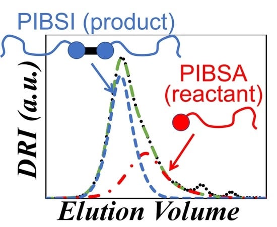
Polymers 15 02350 g002
Figure 3. Plot of the (Polymers 15 02350 i003) DRI trace and (Polymers 15 02350 i004) sum of Gaussians fit of a dehydrated PIBSA sample as a function of elution volume. The contributions of the solvent peaks at 19, 20.5, and 23.5 mL were eliminated in the fitted GPC trace.
Polymers 15 02350 g003
Figure 4. Experimental DRI traces (- - -) from GPC analysis of the PIBSA–H(X) products and their fit with a sum of Gaussians (──) obtained for NAm/NSA ratios of (A) 0.19, (B) 0.38, (C) 0.56, (D) 0.75, (E) 0.94, (F) 1.13, (G) 1.32, and (H) 1.51.
Polymers 15 02350 g004
Figure 5. (A) An example of the quality of (Polymers 15 02350 i004) the fit with a sum of Gaussians for (Polymers 15 02350 i003) the DRI trace of PIBSA–H(0.75), (Polymers 15 02350 i006) the contribution from PIBSA-like molecules, and (Polymers 15 02350 i005) the contribution from non-PIBSA-like molecules. (B) Fits with sums of Gaussians for the PIBSA–H(X) samples with NAm/NSA ratios of (B) (Polymers 15 02350 i007) 0.19, (Polymers 15 02350 i008) 0.38, (Polymers 15 02350 i009) 0.56, (Polymers 15 02350 i010) 0.75, and (Polymers 15 02350 i003) 0.94, and (C) (Polymers 15 02350 i007) 0.94, (Polymers 15 02350 i009) 1.13, (Polymers 15 02350 i010) 1.32, and (Polymers 15 02350 i003) 1.51, normalized to a sum of 1. (D) Plots of the weight fraction (wPLM) of PIBSA-like molecules in the PIBSA–H(X) samples determined by fitting the DRI traces with (×) xgaussSNP and (Polymers 15 02350 i011) linear regression.
Polymers 15 02350 g005
Figure 6. Overlaid DRI contribution of the non-PIBSA fractions of the PIBSA–H(X) samples with NAm/NSA ratios of (A) 0.19, 0.38, 0.56, 0.75, and 0.94, and (B) 0.94, 1.13, 1.32, and 1.51, normalized to a sum of 1. Dashed line: DRI traces of PIBSA.
Polymers 15 02350 g006
Figure 7. Comparison of the fits obtained with (Polymers 15 02350 i007) the xgaussSNP programs and (Polymers 15 02350 i005) the linear regression analysis of the PIBSA–H(X) samples with NAm/NSA ratios of (A) 0.19, (B) 0.38, (C) 0.56, (D) 0.75, (E) 0.94, (F) 1.13, (G) 1.32, and (H) 1.51.
Polymers 15 02350 g007
Figure 8. Weight fraction of (A) PLM obtained (Polymers 15 02350 i011) experimentally from regression of GPC traces (Figure 5D) and with (Polymers 15 02350 i001) reaction3 and (Polymers 15 02350 i012) reaction4, (B) unmaleated PIB obtained with (Polymers 15 02350 i011) reaction3 and (Polymers 15 02350 i001) reaction4, and (C) PLM obtained (Polymers 15 02350 i011) experimentally from regression (Figure 5D) and with (Polymers 15 02350 i001) reaction3 and (Polymers 15 02350 i012) reaction4 after adding a constant wPIB of 0.36.
Polymers 15 02350 g008
Figure 9. Plots of P(M) as a function of molecular weight for (A) the PIB standard with Mn equal to (Polymers 15 02350 i003) 1.0, (Polymers 15 02350 i010) 3.2 kg/mol, and (Polymers 15 02350 i007) PIBSA and (B) simulated MWD for (Polymers 15 02350 i007, P1(M)) m-PIBSI, (Polymers 15 02350 i010, P2(M)) b-PIBSI, (Polymers 15 02350 i005, P3(M)) tri-PIBSI, (Polymers 15 02350 i003, P4(M)) tetra-PIBSI, and (Polymers 15 02350 i013) experimental MWD for higher-order products in the PIBSA–H(0.94) reaction mixture.
Polymers 15 02350 g009
Figure 10. Comparison of (Polymers 15 02350 i007) the simulated DRI traces obtained from the molar fractions obtained with reaction4, wPIB = 0.36, and the DRI traces of PIBSA and b-PIBSI given by the GPC trace obtained for the non-PLM of PIBSA–H(0.94) in Figure 6, and (Polymers 15 02350 i005) the experimental* DRI traces fitted with the xgaussSNP programs of the PIBSA–H(X) products. The NAm/NSA ratios equal (A) 0.19, (B) 0.38, (C) 0.56, (D) 0.75, (E) 0.94, (F) 1.13, (G) 1.32, and (H) 1.51.
Polymers 15 02350 g010aPolymers 15 02350 g010b
Figure 11. Plot of (A) (Polymers 15 02350 i011,×) Mn and (Polymers 15 02350 i014,+) Mw and (B) (Polymers 15 02350 i001,Polymers 15 02350 i012) PDI of the PIBSA–H(X) samples as a function of the NAm/NSA ratio, (Polymers 15 02350 i011,Polymers 15 02350 i014,Polymers 15 02350 i001) simulations, and (×,+,Polymers 15 02350 i012) experiments.
Polymers 15 02350 g011
Disclaimer/Publisher’s Note: The statements, opinions and data contained in all publications are solely those of the individual author(s) and contributor(s) and not of MDPI and/or the editor(s). MDPI and/or the editor(s) disclaim responsibility for any injury to people or property resulting from any ideas, methods, instructions or products referred to in the content.

