
In Situ Detection of Interfacial Flow Instabilities in Polymer Co-Extrusion Using Optical Coherence Tomography and Ultrasonic Techniques

 , ,
, ,
Abstract
:1. Introduction
- In multi-manifold dies, the individual melt streams are fed separately into the extrusion die and are distributed to achieve the desired form. These melt streams are combined just before the die exit, which enables the processing of polymer melts with larger differences in melt temperature and viscosity, but at the cost of lower process flexibility and higher manufacturing costs;
- In the more commonly used feedblock dies, the individual melt streams are combined in an adapter. The multilayer melt stream is then passed to the die for distribution to produce the final shape. With feedblock dies, any number of layers can be processed, but all materials used must have similar melt temperatures and viscosities.
- Viscous encapsulation can result from a viscosity mismatch between the polymers involved; the less viscous melt tends to encapsulate the more viscous melt due to an energetically favored state of minimal pressure loss.
- Elastic layer rearrangement is caused by viscoelastic flow properties of the melts involved. This type of layer distortion is observed even for materials with well-balanced viscosities and for identical melts that are colored differently. The elastic properties of the melt induce secondary flows perpendicular to the main flow direction that give rise to elastic layer rearrangement phenomena. With an increasing ratio of elastic to viscous properties, these phenomena become more pronounced.
- Interfacial flow instabilities are irregularities at the layer interface that result in transient local layer thickness fluctuations [4]. They are commonly categorized into (1) low-frequency wave-type instabilities, (2) high-frequency zig-zag-type instabilities and, occasionally, (3) a transition regime from stable to unstable process behavior. The onset and appearance of these types of instability are strongly dependent on the processing parameters and rheological behavior of the material combination. These interfacial irregularities can be related to products with inferior optical, physical, and mechanical quality, and defects become even more pronounced when a subsequent processing step involves stretching (e.g., blow molding, thermoforming).
- Optical coherence tomography (OCT);
- Ultrasound measurements.
2. Technologies for In Situ Detection of Interfacial Flow Instabilities
2.1. Key Requirements for Co-Extrusion Die and Detection Technology
- Analysis of frozen cross-sections requires adequate sample preparation, and is a time-consuming offline method—which means that information on flow stability is not instantly available—and is therefore unsuitable for process control;
- Visual analysis of the extruded melt stream is the simplest detection method, but requires at least one melt of the co-extrudate to be transparent. It is also biased, since the evaluation depends heavily on the observer and the environment (e.g., ambient light, lighting, and point of observation);
- Visual analysis of the melt flow in the die through optical viewports using various detection systems involves modifications to die geometry and materials (e.g., insertion of lateral silica glass windows), whose effects on co-extrusion flow properties (e.g., wall slippage because the coefficients of friction differ from that of steel) may have to be taken into account. Additionally, a lateral view may lead to misinterpretation, because potential secondary flow effects are most pronounced at the channel edges of flat film flow geometries.
- The measurement system must be applicable to a wide range of material combinations, including amorphous and semicrystalline polymers;
- Material modifications (e.g., by compounding with optically active particles) are to be avoided;
- Detection must be in situ in order to enable real-time evaluation of flow instabilities;
- The detection system must resist thermal load resulting from heat radiation and heat conduction from the die;
- The signal intensity must be sufficient to penetrate through the die wall and the melt stream;
- Adequate depth resolution of the sensor is required to detect low-amplitude instabilities;
- An objective and reliable classification criterion must be developed that quantifies and assesses the stability of the co-extrusion flow;
- The measurement technique must be robust and yield reproducible results.
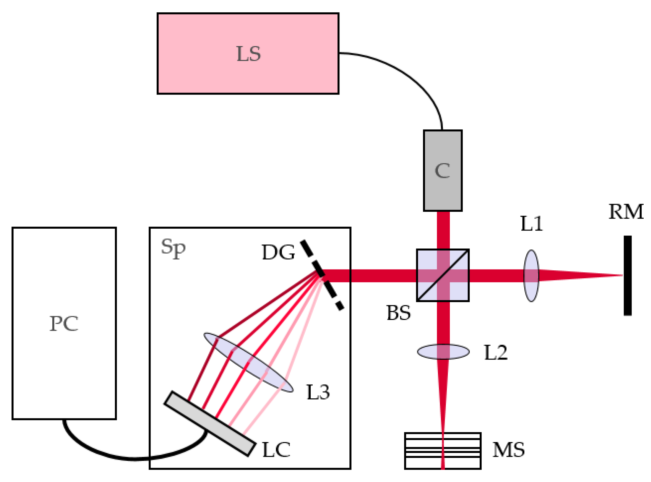
2.2. Optical Coherence Tomography (OCT)
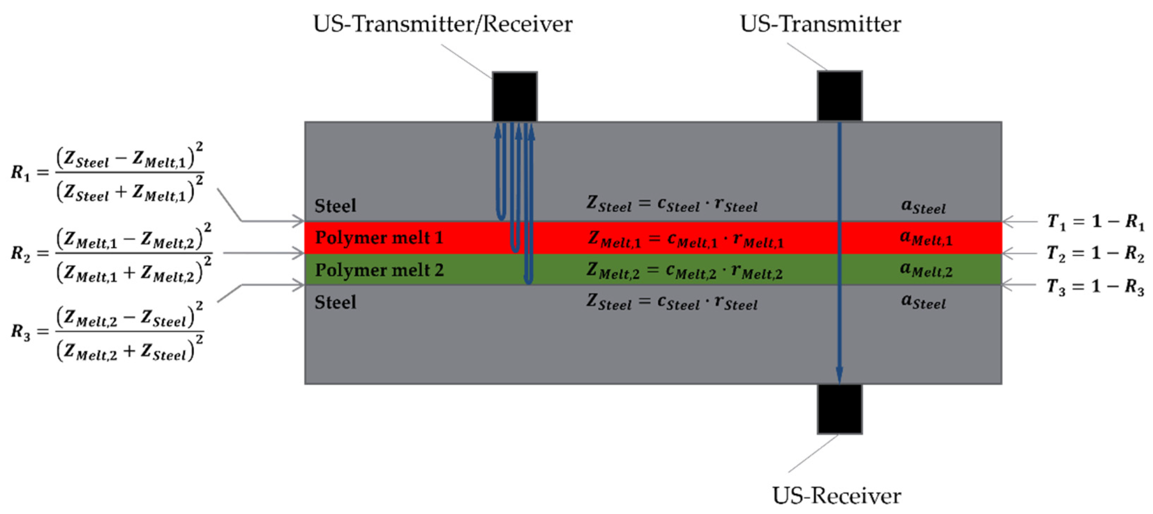
2.3. Ultrasound
3. Experimental
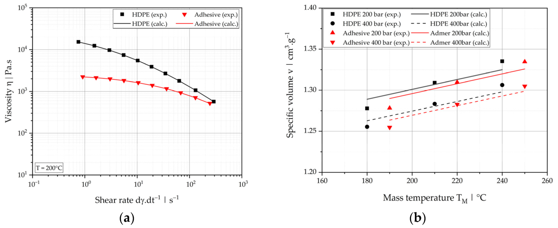
3.1. Materials
3.2. Equipment and Procedure
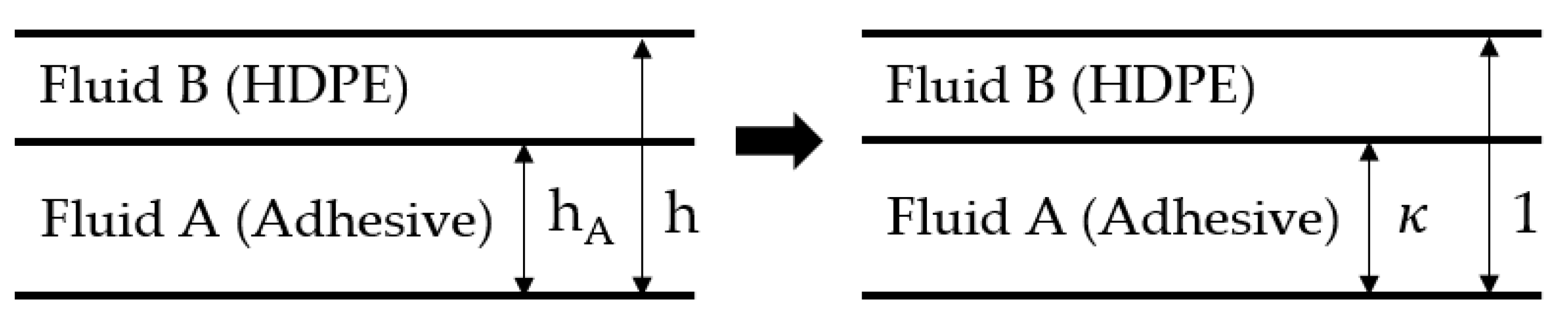
3.3. Flow Modeling
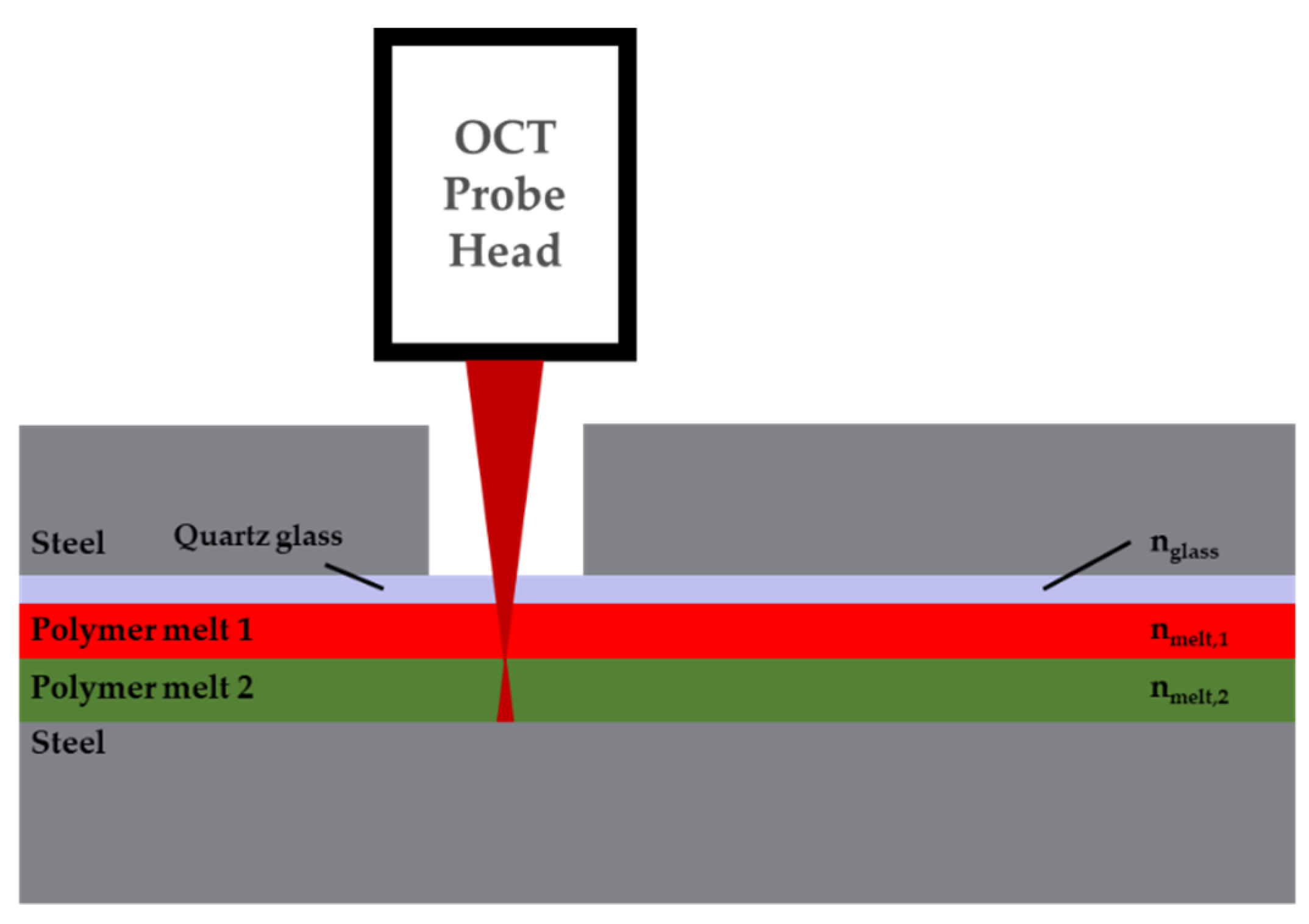
3.4. Approach to Optical Coherence Tomography Measurement
3.5. Ultrasound Measurement Approach
4. Results and Discussion
- Evaluation of the Tait equation (Equation (3)) for each melt on the basis of melt temperature and average pressure within the co-extrusion flow region;
- Transformation of individual and total mass throughputs into corresponding volumetric flow rates;
- Evaluation of average flow velocity and representative shear rate according to Equations (7) and (9);
- Calculation of local power-law parameters from Carreau-Yasuda model parameters for each melt using Equations (10) and (11);
- Calculation of dimensionless input quantities and using Equations (6) and (8);
- Evaluation of the -model (Equation (5)).
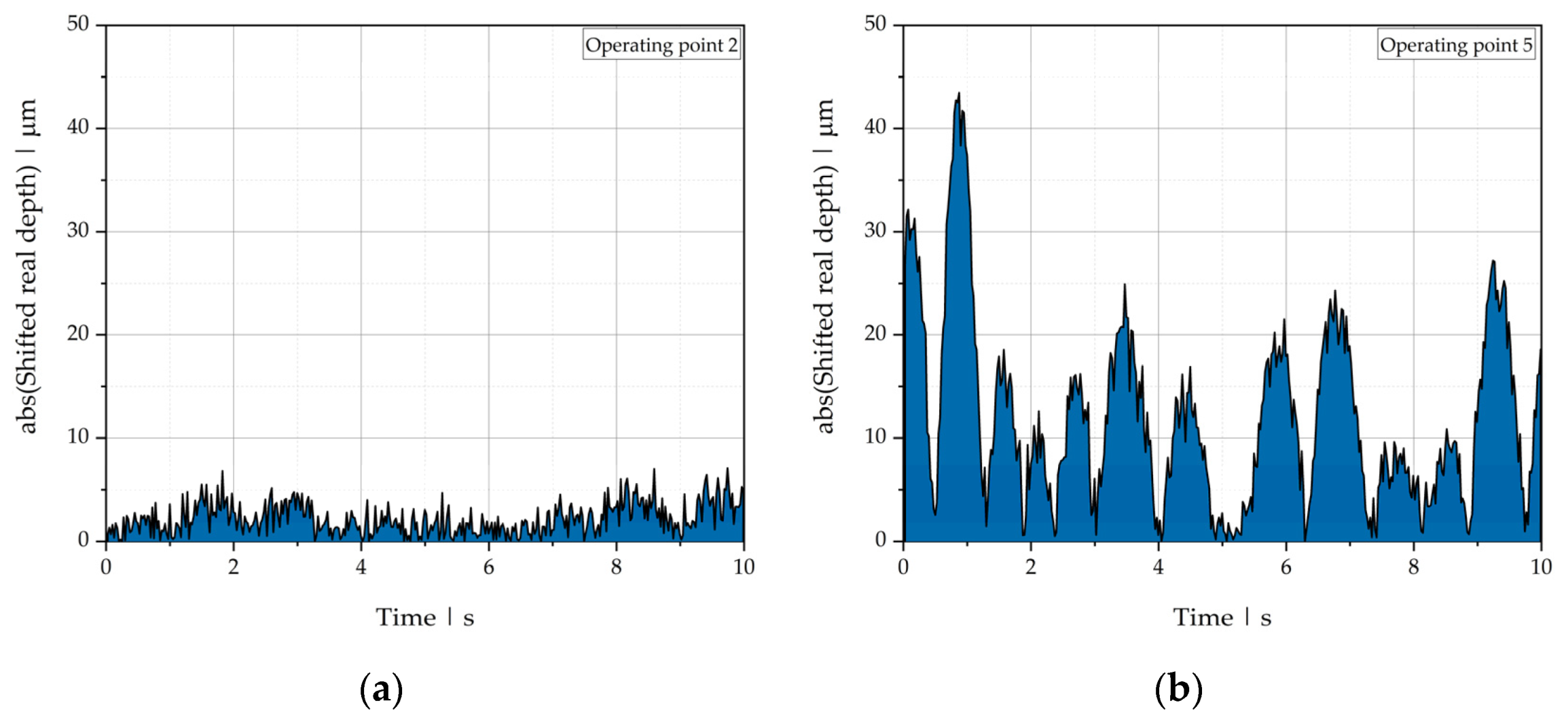
4.1. OCT Measurements
- Standard deviation;
- Signal intensity;
- Number of zero-crossings;
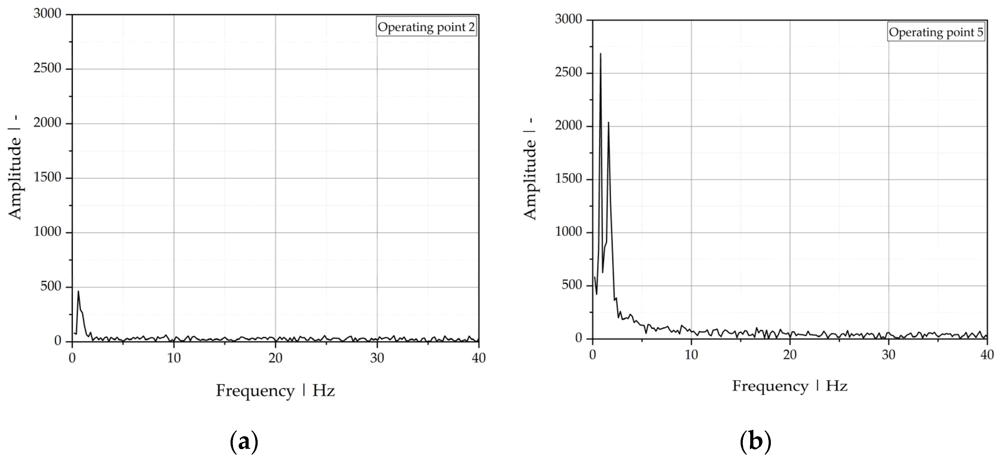
- Amplitude of main frequency by fast Fourier transform (FFT).
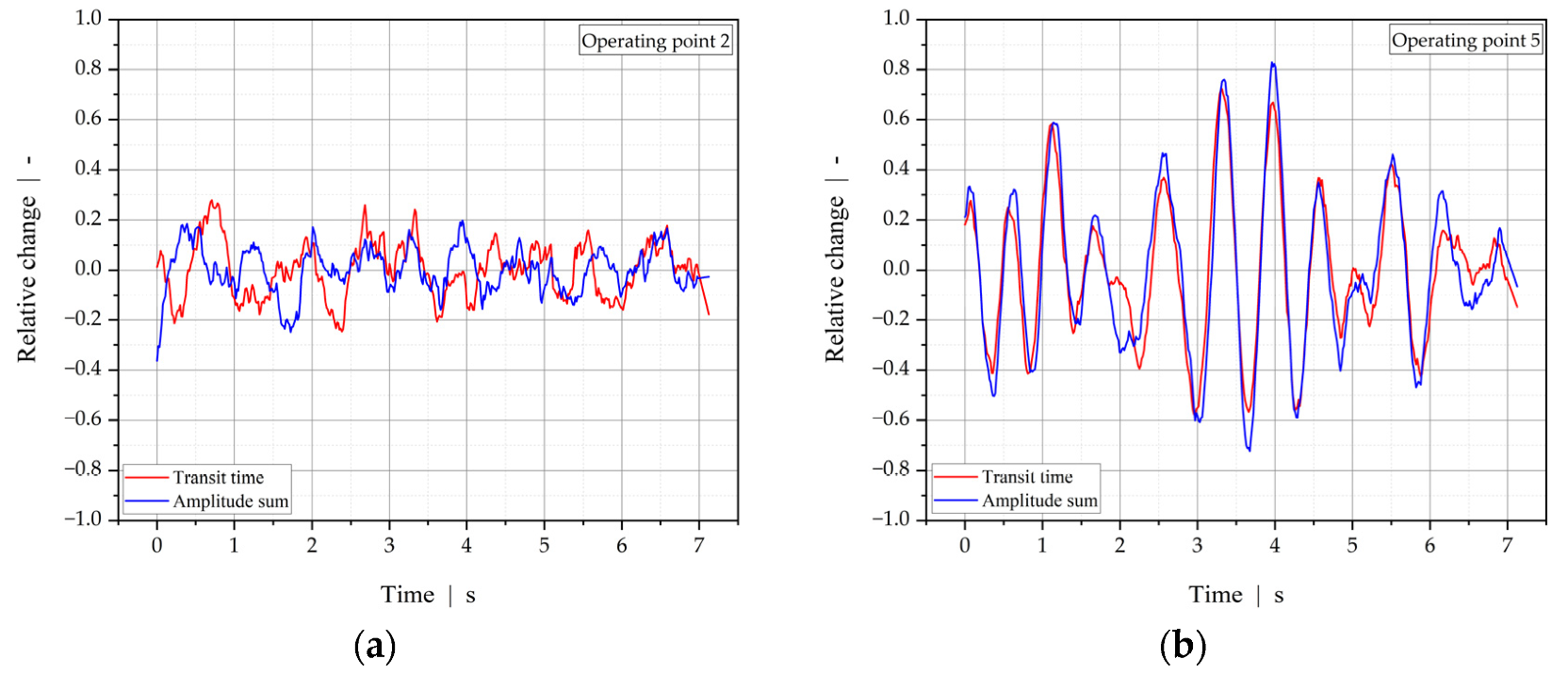
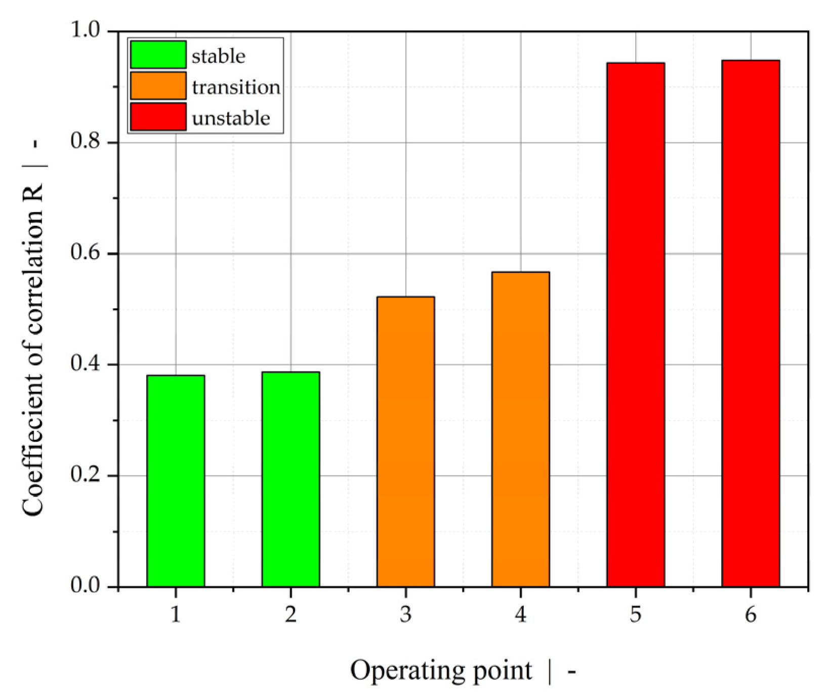
4.2. Ultrasonic Measurements
4.3. Comparison of the Measurement Approaches
5. Conclusions
Author Contributions
Funding
Institutional Review Board Statement
Informed Consent Statement
Data Availability Statement
Conflicts of Interest
References
- Michaeli, W. Extrusion Dies for Plastics and Rubber, 3rd ed.; Hanser Publishers: Munich, Germany, 2003; pp. 236–263. [Google Scholar]
- Dooley, J.; Tung, H. Coextrusion. In Encyclopedia of Polymer Science and Technology, 4th ed.; Mark, H.F., Ed.; John Wiley & Sons Inc.: Hoboken, NJ, USA, 2002; pp. 9–11. [Google Scholar]
- Langhe, D.; Ponting, M. Coextrusion Processing of Multilayered Films. In Manufacturing and Novel Applications of Multilayer Polymer Films, 1st ed.; Ebnesajjad, S., Ed.; Plastics Design Library, Elsevier Inc.: Amsterdam, The Netherlands, 2016; pp. 29–33. [Google Scholar]
- Dooley, J. Coextrusion Instabilities. In Polymer Processing Instabilities, 1st ed.; Hatzikiriakos, S.G., Migler, K.B., Eds.; Marcel Dekker: New York, NY, USA, 2005; pp. 383–426. [Google Scholar]
- Schrenk, W.J.; Bradley, N.L.; Alfrey, T., Jr. Interfacial Flow Instability in Multilayer Coextrusion. Polym. Eng. Sci. 1978, 18, 620–623. [Google Scholar] [CrossRef]
- Han, C.D.; Shetty, R. Studies on Multilayer Film Coextrusion, I. The Rheology of Flat Film Coextrusion. Polym. Eng. Sci. 1976, 16, 697–705. [Google Scholar] [CrossRef]
- Han, C.D.; Shetty, R. Studies on Multilayer Film Coextrusion II. Interfacial Instability in Flat Film Coextrusion. Polym. Eng. Sci. 1978, 18, 180–186. [Google Scholar] [CrossRef]
- Mavridis, H.; Shroff, R.N. Multilayer Extrusion: Experiments and Computer Simulation. Polym. Eng. Sci. 1994, 34, 559–569. [Google Scholar] [CrossRef]
- Bondon, A.; Lamnawar, K.; Maazouz, A. Experimental investigation of a new type of interfacial instability in a reactive extrusion process. Polym. Eng. Sci. 2015, 55, 2542–2552. [Google Scholar] [CrossRef]
- Vuong, S.; Léger, L.; Restagno, F. Controlling interfacial instabilities in PP/EVOH coextruded multilayer films through the surface density of interfacial copolymers. Polym. Eng. Sci. 2020, 60, 1420–1429. [Google Scholar] [CrossRef]
- Tzoganakis, C.; Perdikoulias, J. Interfacial Instabilities in Coextrusion Flows of Low-Density Polyethylenes: Experimental Studies. Polym. Eng. Sci. 2000, 40, 1056–1064. [Google Scholar] [CrossRef]
- Zatloukal, M.; Tzoganakis, C.; Vlček, J.; Sáha, P. Numerical Simulation of Polymer Coextrusion Flows-A Criterion for Detection of “Wave” Interfacial Instability Onset. Int. Polym. Process. 2001, 16, 198–207. [Google Scholar] [CrossRef]
- Zatloukal, M.; Vlček, J.; Tzoganakis, C.; Sáha, P. Viscoelastic Stress Calculation in Multi-Layer Coextrusion Dies: Die Design and Extensional Viscosity Effects On the Onset of ‘Wave’ Interfacial Instabilities. Polym. Eng. Sci. 2002, 42, 1520–1533. [Google Scholar] [CrossRef]
- Zatloukal, M.; Kopytko, W.; Sáha, P.; Martyn, M.; Coates, P.D. Theoretical and experimental investigation of interfacial instability phenomena occurring during viscoelastic coextrusion. Plast. Rubber Compos. 2005, 34, 403–409. [Google Scholar] [CrossRef]
- Zatloukal, M.; Kopytko, W.; Lengálóva, A.; Vlček, J. Theoretical and Experimental Analysis of Interfacial Instabilities in Coextrusion Flows. J. Appl. Polm. Sci. 2005, 98, 153–162. [Google Scholar] [CrossRef]
- Wilson, G.M.; Khomami, B. An experimental investigation of interfacial instabilities in multilayer flow of viscoelastic fluids. J. Non Newt. Fluid Mech. 1992, 45, 355–384. [Google Scholar] [CrossRef]
- Khomami, B.; Ranjbaran, M.M. Experimental studies of interfacial instabilities in multilayer pressure-driven flow of polymeric melts. Rheol. Acta. 1997, 36, 345–366. [Google Scholar] [CrossRef]
- Ganpule, H.K.; Khomami, B. The effect of transient viscoelastic properties on interfacial instabilities in superposed pressure driven channel flows. J. Non Newt. Fluid Mech. 1999, 80, 217–249. [Google Scholar] [CrossRef]
- Martyn, M.T.; Spares, R.; Coates, P.D.; Zatloukal, M. Imaging and analysis of wave type interfacial instability in the coextrusion of low-density polyethylene melts. J. Non Newt. Fluid Mech. 2009, 156, 150–164. [Google Scholar] [CrossRef]
- Martyn, M.T.; Coates, P.D.; Zatloukal, M. Influence of coextrusion die channel height on interfacial instability of low density polyethylene melt flow. Plast. Rubber Compos. 2014, 43, 25–31. [Google Scholar] [CrossRef]
- Zhang, H.; Lamnawar, K.; Maazouz, A. Role of the interphase in the interfacial flow stability in coextrusion of compatible multilayered polymers. Key Eng. Mater. 2013, 554–557, 1738–1750. [Google Scholar] [CrossRef]
- Huang, D.; Swanson, E.A.; Lin, C.P.; Schuman, J.S.; Stinson, W.G.; Chang, W.; Hee, M.R.; Flotte, T.; Gregory, K.; Puliafito, C.A.; et al. Optical coherence tomography. Science 1991, 254, 1178–1181. [Google Scholar] [CrossRef] [PubMed] [Green Version]
- Fercher, A.F.; Hitzenberger, C.K.; Drexler, W.; Kamp, G.; Sattmann, H. In vivo optical coherence tomography. Am. J. Ophthalmol. 1993, 116, 113–114. [Google Scholar] [CrossRef]
- Fujimoto, J.G.; Drexler, W.; Schuman, J.S.; Hitzenberger, C.K. Optical Coherence Tomography (OCT) in ophthalmology: Introduction. Opt. Express 2009, 17, 3978–3979. [Google Scholar] [CrossRef]
- Welzel, J.; Lankenau, E.; Hüttmann, G.; Birngruber, R. OCT in Dermatology. In Optical Coherence Tomography. Biological and Medical Physics, Biomedical Engineering; Drexler, W., Fujimoto, J.G., Eds.; Springer: Berlin Heidelberg, Germany, 2008; Volume 1, pp. 1103–1122. [Google Scholar]
- Stifter, D. Beyond biomedicine: A review of alternative applications and developments for optical coherence tomography. Appl. Phys. B 2007, 88, 337–357. [Google Scholar] [CrossRef]
- Golde, J.; Kirsten, L.; Schnabel, C.; Walther, J.; Koch, E. Optical Coherence Tomography for NDE. In Handbook of Advanced Nondestructive Evaluation; Ida, N., Meyendorf, N., Eds.; Springer: Cham, Switzerland, 2019; Volume 1, pp. 469–511. [Google Scholar]
- Markl, D.; Hannesschläger, G.; Sacher, S.; Leitner, M.; Khinast, J.G.; Buchsbaum, A. Automated pharmaceutical tablet coating layer evaluation of optical coherence tomography images. Meas. Sci. Technol. 2015, 26, 035701. [Google Scholar] [CrossRef]
- Mittelstädt, C.; Mattulat, T.; Seefeld, T.; Kogel-Hollacher, M. Novel approach for weld depth determination using optical coherence tomography measurement in laser deep penetration welding of aluminum and steel. J. Laser Appl. 2019, 31, 022007. [Google Scholar] [CrossRef]
- Praher, B.; Straka, K.; Steinbichler, G. An ultrasound-based system for temperature distribution measurements in injection moulding: System design, simulations and off-line test measurements in water. Meas. Sci. Technol. 2013, 24, 084004. [Google Scholar] [CrossRef]
- Praher, B.; Goldmann, M.; Steinbichler, G. Inline melt homogeneity measurement in injection molding. AIP Conf. Proc. 2019, 2055, 120006. [Google Scholar]
- Altmann, D.; Praher, B.; Steinbichler, G. Simulation of the melting behavior in an injection molding plasticizing unit as measured by pressure and ultrasound measurement technology. AIP Conf. Proc. 2019, 2055, 040003. [Google Scholar]
- Aigner, M.; Praher, B.; Kneidinger, C.; Miethlinger, J.; Steinbichler, G. Verifying the melting behavior in single-screw plasticization units using a novel simulation model and experimental method. Int. Polym. Process. 2014, 29, 624–634. [Google Scholar] [CrossRef]
- Kažys, R.; Rekuvienė, R. Viscosity and density measurement methods for polymer melts. Ultrasound 2011, 66, 20–25. [Google Scholar] [CrossRef] [Green Version]
- Praher, B.; Steinbichler, G. Ultrasound-based measurement of liquid-layer thickness: A novel time-domain approach. Mech. Syst. Signal Process. 2017, 82, 166–177. [Google Scholar] [CrossRef]
- LyondellBasell. Available online: https://www.lyondellbasell.com/en/polymers/p/Hostalen-ACP-5831-D/af08fe40-b138-4201-ac3d-2be8113e8024 (accessed on 21 August 2021).
- Mitsui Chemicals Group-Admer. Available online: https://admer.eu/media/product_sheets/ (accessed on 21 August 2021).
- Rathner, R.; Roland, W.; Albrecht, H.; Ruemer, F.; Miethlinger, J. Applicability of the Cox-Merz Rule to High-Density Polyethylene Materials with Various Molecular Masses. Polymers 2021, 13, 1218. [Google Scholar] [CrossRef]
- Carreau, P.J. Rheological Equations from Molecular Network Theories. Ph.D. Thesis, University of Wisconsin-Madison, Madison, WI, USA, 1968. [Google Scholar]
- Yasuda, K. Investigation of the Analogies between Viscometric and Linear Viscoelastic Properties of Polystyrene. Ph.D. Thesis, MIT, Cambridge, MA, USA, 1979. [Google Scholar]
- Tait, P.G. Report on some of the Physical Properties of Fresh Water and of Sea-Water. Phys. Chem. 1888, 2, 1–76. [Google Scholar]
- Osswald, T.A.; Hernandez-Ortiz, J.P. Polymer Processing: Modeling and Simulation; Hanser Publisher: Munich, Germany, 2002; pp. 47–50. ISBN 978-1569903988. [Google Scholar]
- Hammer, A.; Roland, W.; Marschik, C.; Steinbichler, G. Applying the Shooting Method to Predict the Co-extrusion Flow of Non-Newtonian Fluids Through Rectangular Ducts. In Proceedings of the SPE ANTEC Tech. Paper, May 2021; Available online: https://www.researchgate.net/publication/351839393 (accessed on 23 August 2021).
- Hammer, A.; Roland, W.; Marschik, C.; Steinbichler, G. Predicting the Co-extrusion Flow of Non-Newtonian Fluids Through Rectangular Ducts-a Hybrid Modeling Approach. J. Non. Newt. Fluid Mech. 2021, 295, 104618. [Google Scholar] [CrossRef]
- Smith, D.R.; Loewenstein, E.V. Optical constants of far infrared materials. 3: Plastics. Appl. Opt. 1975, 14, 1335–1341. [Google Scholar] [CrossRef] [PubMed]
- MATLAB Release 2018b; The Math Works, Inc.: Natick, MA, USA, 2018.
- Schober, P.; Boer, C.; Lothar, A.S. Correlation Coefficients: Appropriate Use and Interpretation. Anesth. Analg. 2018, 126, 1763–1768. [Google Scholar] [CrossRef]


| Type | Grade | Supplier | Application | Density (ISO 1183) | MFR (ISO 1133) |
|---|---|---|---|---|---|
| HDPE | Hostalen ACP5831D | Lyondell Basell | Blow molding | 0.958 g·cm−3 | 0.25 g/10 min (190 °C/2.16 kg) |
| Adhesive | Admer NF408E | Mitsui Chemicals | Adhesive resin | 0.920 g·cm−3 | 1.60 g/10 min (190 °C/2.16 kg) |
| Parameter | Unit | HDPE ACP5831D | Adhesive NF408E |
|---|---|---|---|
| - | 1.057 × 10⁻⁴ | 1.572 × 10⁻⁴ | |
| a | - | 3.982 × 10⁻¹ | 4.876 × 10⁻¹ |
| Pa·s | 3.474 × 10⁴ | 6.060 × 10³ | |
| Pa·s | 0 | 0 | |
| s | 1.203 × 10⁻¹ | 1.029 × 10⁻² | |
| α | - | 1.224 × 10⁻² | 1.633 × 10⁻² |
| T0 | K | 473.15 | 473.15 |
| Parameter | Unit | HDPE ACP5831D | Adhesive NF408E |
|---|---|---|---|
| m3·kg−1 | 1.43 × 10⁻³ | 1.39 × 10⁻³ | |
| m·(kg·K)−1 | 6.18 × 10⁻⁷ | 6.18 × 10⁻⁷ | |
| Pa | 6.00 × 10⁷ | 6.00 × 10⁷ | |
| K−1 | 6.49 × 10⁻⁵ | 6.49 × 10⁻⁵ | |
| K | 622.28 | 573.15 |
| Material | Unit | B1 | B2 | B3 | A | TDie |
|---|---|---|---|---|---|---|
| HDPE ACP581D | °C | 180 | 190 | 190 | 190 | 200 |
| Adhesive NF408E | °C | 190 | 200 | 200 | 200 |
| Operating Point | Screw Speed | rpm | |
|---|---|---|
| Adhesive NF408E | HDPE ACP5831D | |
| 1 | 14.2 | 12 |
| 2 | 16.2 | 9.8 |
| 3 | 17.0 | 9.0 |
| 4 | 17.5 | 8.5 |
| 5 | 28.0 | 8.0 |
| 6 | 48.0 | 8.0 |
| Parameter | Unit | Value |
|---|---|---|
| Center wavelength | nm | 1300 |
| Line rate (A-scan rate, typical) | kHz | 28 |
| Axial resolution (depth resolution) | µm | 7.5 |
| Lateral resolution | µm | 15 |
| Maximum field of view | mm | 10 × 10 × 2.54 |
| Maximum pixels per A-scan | - | 512 |
| Sensitivity (typical) | dB | 102 |
| Operating Point | Mass Throughput | kg·h−1 | Position of Interface | - | Stability | +/~/-/-- | ||
|---|---|---|---|---|---|
| Adhesive NF408E | HDPE ACP5831D | Total | Adhesive HDPE | Adhesive HDPE | |
| 1 | 1.62 | 1.18 | 2.80 | 0.523 | + |
| 2 | 1.84 | 0.97 | 2.80 | 0.571 | + |
| 3 | 1.94 | 0.88 | 2.81 | 0.593 | ~ |
| 4 | 1.99 | 0.82 | 2.82 | 0.606 | ~ |
| 5 | 3.16 | 0.74 | 3.90 | 0.691 | - |
| 6 | 5.35 | 0.71 | 6.06 | 0.763 | -- |
| Material | Refractive index | - | |
|---|---|---|
| Mean | STD | |
| Adhesive NF408E | 1.375 | 0.00109 |
| HDPE ACP581D | 1.387 | 0.00194 |
| Class Label | Standard Deviation | µm | Signal Intensity | µm2 | Number of Zero-Crossings | - | Magnitude Main Frequency | - | ||||
|---|---|---|---|---|---|---|---|---|
| Min. | Max. | Min. | Max. | Min. | Max. | Min. | Max. | |
| Stable | <3 | <1000 | >100 | <500 | ||||
| Transition | 3 | 6 | 1000 | 2500 | 30 | 100 | 500 | 1000 |
| Unstable | 6 | 50 | 2500 | 20,000 | 15 | 30 | 1000 | 10,000 |
| Highly unstable | >50 | >20,000 | <15 | >10,000 | ||||
| Parameter | OCT | Ultrasonic | Visual |
|---|---|---|---|
| Determination of interface position | Possible; requires refractive indices of melts | Not possible | Not possible |
| Measurement position | Optical viewport required | Flexible | Assessment of co-extrudate at die outlet |
| Coupling of sensor probe | Contactless | Direct coupling to steel body required | - |
| Limitations in terms of material properties | Optical transparency at wavelength of OCT required; high sensitivity regarding differences in optical properties | Indirect measurement necessary because impedances of polymers are often highly similar | Transparent materials required (at wavelength of visible light) |
| Investment costs | High | Low | None |
| Potential for integration into industrial processes | Robust, unbiased results, real-time evaluation possible | Robust, unbiased results, real-time evaluation possible | Observer-dependent results |
| Data amount | High (B-scans, depends on sampling rate) | Medium (depends on sampling rate) | None; no direct quantification possible |
Publisher’s Note: MDPI stays neutral with regard to jurisdictional claims in published maps and institutional affiliations. |
© 2021 by the authors. Licensee MDPI, Basel, Switzerland. This article is an open access article distributed under the terms and conditions of the Creative Commons Attribution (CC BY) license (https://creativecommons.org/licenses/by/4.0/).
Share and Cite
Hammer, A.; Roland, W.; Zacher, M.; Praher, B.; Hannesschläger, G.; Löw-Baselli, B.; Steinbichler, G. In Situ Detection of Interfacial Flow Instabilities in Polymer Co-Extrusion Using Optical Coherence Tomography and Ultrasonic Techniques. Polymers 2021, 13, 2880. https://doi.org/10.3390/polym13172880
Hammer A, Roland W, Zacher M, Praher B, Hannesschläger G, Löw-Baselli B, Steinbichler G. In Situ Detection of Interfacial Flow Instabilities in Polymer Co-Extrusion Using Optical Coherence Tomography and Ultrasonic Techniques. Polymers. 2021; 13(17):2880. https://doi.org/10.3390/polym13172880
Chicago/Turabian StyleHammer, Alexander, Wolfgang Roland, Maximilian Zacher, Bernhard Praher, Günther Hannesschläger, Bernhard Löw-Baselli, and Georg Steinbichler. 2021. "In Situ Detection of Interfacial Flow Instabilities in Polymer Co-Extrusion Using Optical Coherence Tomography and Ultrasonic Techniques" Polymers 13, no. 17: 2880. https://doi.org/10.3390/polym13172880