Aperiodic Photonics of Elliptic Curves

Abstract

In this paper we propose a novel approach to aperiodic order in optical science and technology that leverages the intrinsic structural complexity of certain non-polynomial (hard) problems in number theory and cryptography for the engineering of optical media with novel transport and wave localization properties. In particular, we address structure-property relationships in a large number (900) of light scattering systems that physically manifest the distinctive aperiodic order of elliptic curves and the associated discrete logarithm problem over finite fields. Besides defining an extremely rich subject with profound connections to diverse mathematical areas, elliptic curves offer unprecedented opportunities to engineer light scattering phenomena in aperiodic environments beyond the limitations of traditional random media. Our theoretical analysis combines the interdisciplinary methods of point patterns spatial statistics with the rigorous Green’s matrix solution of the multiple wave scattering problem for electric and magnetic dipoles and provides access to the spectral and light scattering properties of novel deterministic aperiodic structures with enhanced light-matter coupling for nanophotonics and metamaterials applications to imaging and spectroscopy.

1. Introduction

Stimulated by P. W. Anderson’s realization that strong disorder can inhibit electronic transport [1], the study of quantum and classical waves in disordered media with randomly fluctuating potentials has unveiled profound analogies between the electronic and the optical behavior of complex materials [2,3,4,5]. Moreover, understanding wave transport and localization phenomena in aperiodic optical media provides opportunities to tailor their optical density of states and to enhance light-matter interactions for the engineering of novel active photonic devices. Specifically, the study of multiple light scattering in random media led to the demonstration of random lasers with both uniform [6,7,8,9,10] and correlated disorder [11], as well as to remarkable advances in optical imaging [12,13,14,15,16] and spectroscopy [17,18]. However, despite a sustained research effort, Anderson localization of optical waves remains an elusive phenomenon since it does not occur in open-scattering random media when the vector nature of light is taken into account.

The lack of Anderson localization in optical random media is attributed to the detrimental effects of near-field coupling of electromagnetic waves confined at the sub-wavelength scale between scatterers in dense systems [19,20,21]. Due to the uncorrelated nature of the disorder, it is difficult to overcome this problem and to establish simple design rules for the optimization of uniform random media, often limiting their applications to optical device engineering. As a result, there is currently a compelling need to develop optical media that are deterministic in nature, while at the same time sufficiently structurally-complex to offer an alternative route to achieve stronger light localization effects compared to uniform random systems. In response to these challenges, deterministic aperiodic structures have been developed. Deterministic structures with aperiodic though long-range ordered distributions of scattering potentials have a long history in the electronics and optics communities due to significant advantages in design and compatibility with standard fabrication technologies compared to random systems [22,23]. These structures manifest unique spectral characteristics that lead to physical properties that cannot be found in either periodic or uniform random media, such as multifractal density of eigenstates with varying degrees of spatial localization, known as critical modes [24,25,26,27,28], anomalous photon transport regimes [29,30], and distinctive wave localization transitions [31,32]. Critical modes feature highly-fragmented envelopes characterized by local power-law scaling that reflects the multi-scale geometry of certain deterministic aperiodic potentials that found recent applications to light emission and lasing, optical sensing, photo-detection, and nonlinear optical devices [24,26,33,34,35,36,37,38,39,40,41]. An alternative strategy relies on the engineering of scattering structures based on the distinctive aperiodic order, unpredictability, and complexity that naturally arise in the context of number theory [23,42,43]. This profound and deeply-fascinating field of mathematics provides paradigmatic examples of the subtle interplay between structure and randomness [44,45]. Examples include the aperiodic distribution of prime numbers and their algebraic field generalizations, the almost-periodicity characteristic of arithmetic functions, aperiodic primitive roots and quadratic residue sequences, the intricate behavior of Dirichlet L-functions (which include the Riemann’s $\zeta$ function), and the distribution of binary digits in Galois fields, just to name a few.

In this paper, we introduce a novel class of deterministic structures that manifest the distinctive aperiodic order of elliptic curves and the associated discrete logarithm problem over finite fields. In particular, using the Green’s matrix formalism we systematically study the spectral and localization properties of their scattering resonances with respect to uniform random systems and we address distinctive structure-property relationships using the methods of point patterns spatial analysis. Finally, we present an extension of the coupled electric dipole method that includes the scattering contribution of magnetic modes, which are important for the accurate design of aperiodic arrays with finite-size dielectric nanoparticles. Specifically, we apply our method to the study of the scattering spectra and the forward/backward scattering response of elliptic curves and discrete logarithm structures composed of TiO${}_2$ nanoparticles of sub-wavelength dimensions.

Our results demonstrate that the light scattering properties of particle arrays designed according to the proposed elliptic curve approach are distinctively different from the ones of uniform random systems, despite close similarities are observed in both point pattern and spectral statistics. Based on the analysis of 900 different structures, we show that at small values of optical density the distributions of the level spacing of the complex resonances of elliptic curve structures (and of their discrete logarithm) is described by critical statistics, differently from the usual case of diffusive transport regime encountered in uniform random systems. Random systems exhibit critical statistics only at the density corresponding to the localization threshold, where all the eigenmodes are known to exhibit fractal scaling [46]. In contrast, here we show numerically that elliptic curve structures display critical spectral statistics over a large range of densities until they transition into a more localized transport regime described by Poisson statistics at very large densities. Our comprehensive analysis also indicates that elliptic curve structures feature a much smaller fraction of sub-radiant proximity resonances compared to traditional random systems, resulting in significantly increased modal lifetimes and enhanced light-matter coupling. Finally, we design an elliptic curve and discrete logarithm arrays of TiO${}_2$ nanoparticles with a resonant scattering across the visible spectrum and demonstrate a large tunability of the spectral width of their back-scattered radiation.

Our findings not only underline the importance of structural correlations in elliptic curve-based structures for the improvement of photonic systems but also show that the solution of the associated wave scattering problem reveals remarkable differences in the scattering and localization properties that may become important for the optical identification of vulnerabilities in elliptic-curve cryptosystems.

2. Elliptic Curves and Discrete Logarithm Structures

An elliptic curve $E\left(\mathbb{K}\right)$ over a number field $\mathbb{K}$ is a non-singular curve (i.e., with a unique tangent at every point) with points in $\mathbb{K}$ that are the solutions of a cubic equation. Therefore, elliptic curves can be thought of as the set of solutions in the field $\mathbb{K}$ of equations in the form [47]:

$$y^2=x^3+Ax+B,$$

(1)

where the coefficients A and B belong to $\mathbb{K}$ and satisfy the non-singular condition ${\Delta }_E=4A^3+27B^2\ne 0$ for the discriminant ${\Delta }_E$ that excludes cusps or self-intersections (i.e., knots) [47,48]. Elliptic curves specified as in the equation above are said to be given in the Weierstrass normal form. 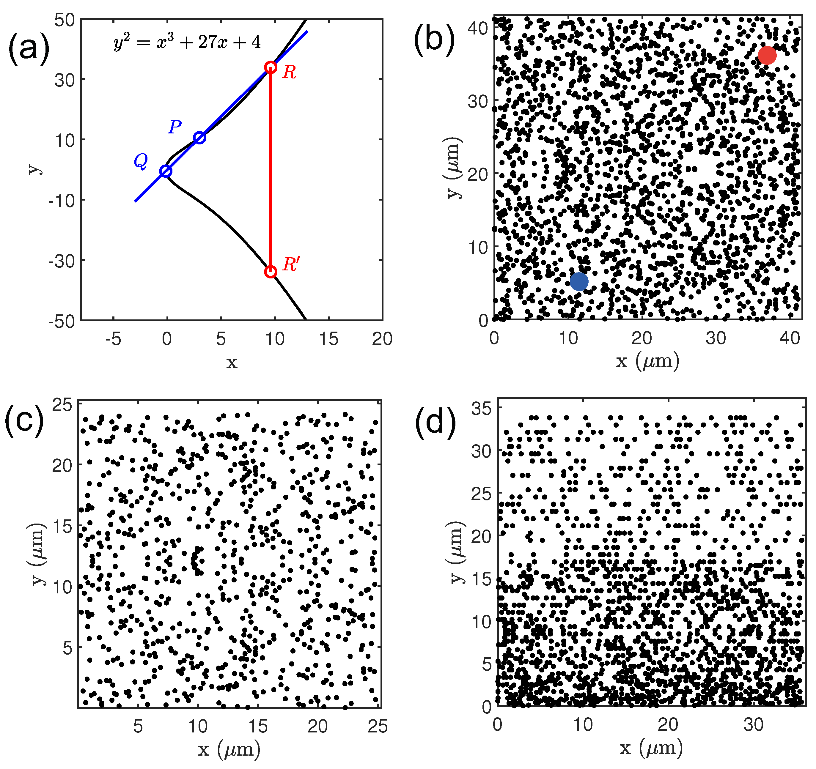When $\mathbb{K}$ coincides with the set of real numbers $\mathbb{R}$, we can graph $E\left(\mathbb{R}\right)$ and view its solutions $(x,y)$ as actual points of a plane curve. An example is shown in Figure 1a for a representative elliptic curve ($EC$) over the real numbers defined by the parameters $A=27$ and $B=4$. Clearly, different choices for the field $\mathbb{K}$ will result in different sets of solutions for the same cubic equation, since elliptic curves can also be regarded as particular examples of algebraic varieties. Algebraic varieties over the field of rational numbers $\mathbb{Q}$ have been investigated already by post-classical Greek mathematicians, most notably by Diophantus, who lived around 270 $CE$ in Alexandria, Egypt. In his honor, we refer to a polynomial equation in one or more variables whose solutions are sought among the integers or rational numbers as a ‘Diophantine equation’. The history of Diophantine equations and elliptic curves runs central to the development of the most advanced ideas of number theory that led to the proof of the celebrated Fermat’s last theorem by the British mathematician Andrew Wiles in 1995 [49].

The study of elliptic curves constitutes a major area of current research in number theory with important applications to cryptography and integer factorization. Interestingly, when endowed with an extra point $\mathcal{O}$ at infinity, the points of elliptic curves acquire the structure of an Abelian group with the point $\mathcal{O}$ serving as the neutral group element. In particular, the group of rational points (solutions in $\mathbb{Q}$) of the elliptic curve $E\left(\mathbb{Q}\right)$ is finitely generated (Mordell’s theorem) and can be decomposed into the direct sum of $\mathbb{Z}$ with finite cyclic groups [47,48]. More specifically, one can also show the group of rational points has the form: $E\left(\mathbb{Q}\right)\cong T⨁{\mathbb{Z}}^r$ where T is a finite group consisting of torsion points (i.e., a point $P\in E$ satisfying $mP=\mathcal{O}$ is called a point of order m in the group E. All points of finite order form an Abelian subgroup called the torsion group of E) and r is a non-negative number, called the algebraic rank of the elliptic curve E, which somehow characterizes its size [48,50].

An example of the composition group law for the previously introduced elliptic curve over the real numbers is illustrated in Figure 1a where two points with real-valued coordinates P and Q are summed to obtain the point $R^{\prime }$. The simplest way to introduce the group composition law is to implement the following geometrical construction [47,48]: we first draw the line that intersects P and Q. This line will generally intersect the cubic at a third point, called R. We then define the addition $P+Q$ as the point $-R$, i.e., the point opposite R. It is possible to prove that this definition for addition works except in a few special cases related to the point at infinity and intersection multiplicity [47,48].

The type of elliptic curves that we will investigate in this paper are defined over the finite field ${\mathbb{F}}_p\equiv \mathbb{Z}/p\mathbb{Z}$ where p is an odd prime number. This is the set of integers modulo p, which is an algebraic field when p is prime. An elliptic curve over ${\mathbb{F}}_p$ is still defined by Equation (1) where the equal sign is replaced by the congruence operation:

$$y^2\equiv x^3+Ax+Bmodp$$

(2)

where the coefficients $A,B\in {\mathbb{F}}_p$ and the discriminant ${\Delta }_E$ in this case must be incongruent to 0 when reduced modulo the prime p. Since ${\mathbb{F}}_p$ is a finite group with p elements, the elliptic curve defined above has only a finite number of points which we expect to be approximately $p+1$ in number (remember the necessity to add the extra point at infinity). It turns out that the actual number of points $N_p$ of the curve $E\left({\mathbb{F}}_p\right)$ fluctuates from $p+1$ within a bound $2\sqrt{p}$, which is a result proved in 1933 by Helmut Hesse. More precisely, if we define the quantity $a_p=p+1-N_p$ Hesse’s theorem states that $|a_p|\le 2\sqrt{p}$ [47,48]. One of the most challenging yet unsolved problems in mathematics, which is also a millennium prize problem of the Clay Mathematics Institute [51], is the Birch and Swinnerton-Dyer conjecture (BSD) that identifies the algebraic and the analytic rank of an elliptic curve [48,52]. The analytic rank of a curve E is equal to the order of vanishing of the associated Dirichlet L-function $L(E,s)$ at $s=1$. The L-function $L(E,s)$ mentioned above is a complex-valued function that is constructed based on the numbers $a_p$ [53]. This function, which is analogous to the Riemann zeta function $\zeta$ and the Dirichlet L-series, can be analytically continued over the whole complex plane and it encodes information on the number of solutions of E modulo a prime onto the properties of the associated complex function $L(E,s)$. Moreover, $L(E,s)$ satisfies a Riemann-type functional equation connecting its values $L(E,s)$ and $L(E,2-s)$ for any s. According to the Sato–Tate conjecture, the random looking fluctuations observed in the ‘error term’ $a_p$ when the prime p is varied are captured by a ‘sine-squared’ probability distribution. This conjecture has been proved in 2008 by Richard Taylor limited to particular types of elliptic curves [54].

In Figure 1b we show the elliptic curve over ${\mathbb{F}}_p$ with $p=2111$ that has the same parameters as the curve $E\left(\mathbb{R}\right)$ previously shown in Figure 1a. We note that the curve has been rescaled by a constant parameter so that the average separation between points equals 450 nm, which enables resonant scattering responses across the visible spectrum. Apart from this irrelevant scaling, the points on this curve appear to be randomly distributed in stark contrast with its counterpart defined over the field of real numbers. Moreover, working with $EC$ over finite fields allows one to define the associated discrete logarithm problem that plays an essential role in elliptic curves cryptography due to its non-polynomial complexity [47,50]. Let $EC$ be an elliptic curve over ${\mathbb{F}}_p$ (see Figure 1b) and M (blue circle marker) and W (red circle marker) two points on the curve. The discrete logarithm problem is the problem of finding an integer k such that $W=kM$. By fixing a starting point W and applying this group operation repeatedly to all the points M on the curve E in Figure 1b, we can obtain the point patterns shown in Figure 1c,d, which are the physical representations of the abstract discrete logarithm problem on the original curve E. Specifically, Figure 1c,d display curves characterized by the coordinates $(M_x;k)$ and $(M_y;k)$ rescaled in order to have an average interparticle separtion equal to 450 nm, respectively. These types of aperiodic deterministic structures are referred to as the elliptic curve discrete logarithm ($EC$$DL$). Clearly, the distribution of points in $EC$$DL$ strongly depends on the choice of the initial point W on the starting $EC$. In our work we have uniformly sampled 9 starting points on E. We have found that the resulting $EC$$DL$ curves can be divided into two main categories: $EC$$DL$ point patterns that are symmetric with respect to the x-axis (Figure 1c) and others that do not show this structural symmetry and are generally less homogeneous (Figure 1d). Moreover, the number of elements $EC$$DL$ cannot be controlled exactly because it depends on the value of the integer k. The complexity of the discrete logarithm problem for elliptic curves over finite fields is at the heart elliptic-curve cryptography (ECC), which is the most advanced approach to public-key cryptography that protects highly secure communications (up to to-secret classification) using key that are significantly smaller compared to alternative methods such as RSA-based cryptosystems [47,50]. In what follow we will apply the statistical methods of point pattern analysis and the theory of multiple light scattering in order to investigate the structural, spectral, and scattering properties of these number-theoretic structures regarded as aperiodic photonic systems of scattering point-particles.

3. Structural and Spectral Properties of Elliptic Curves and Discrete Logarithm Arrays

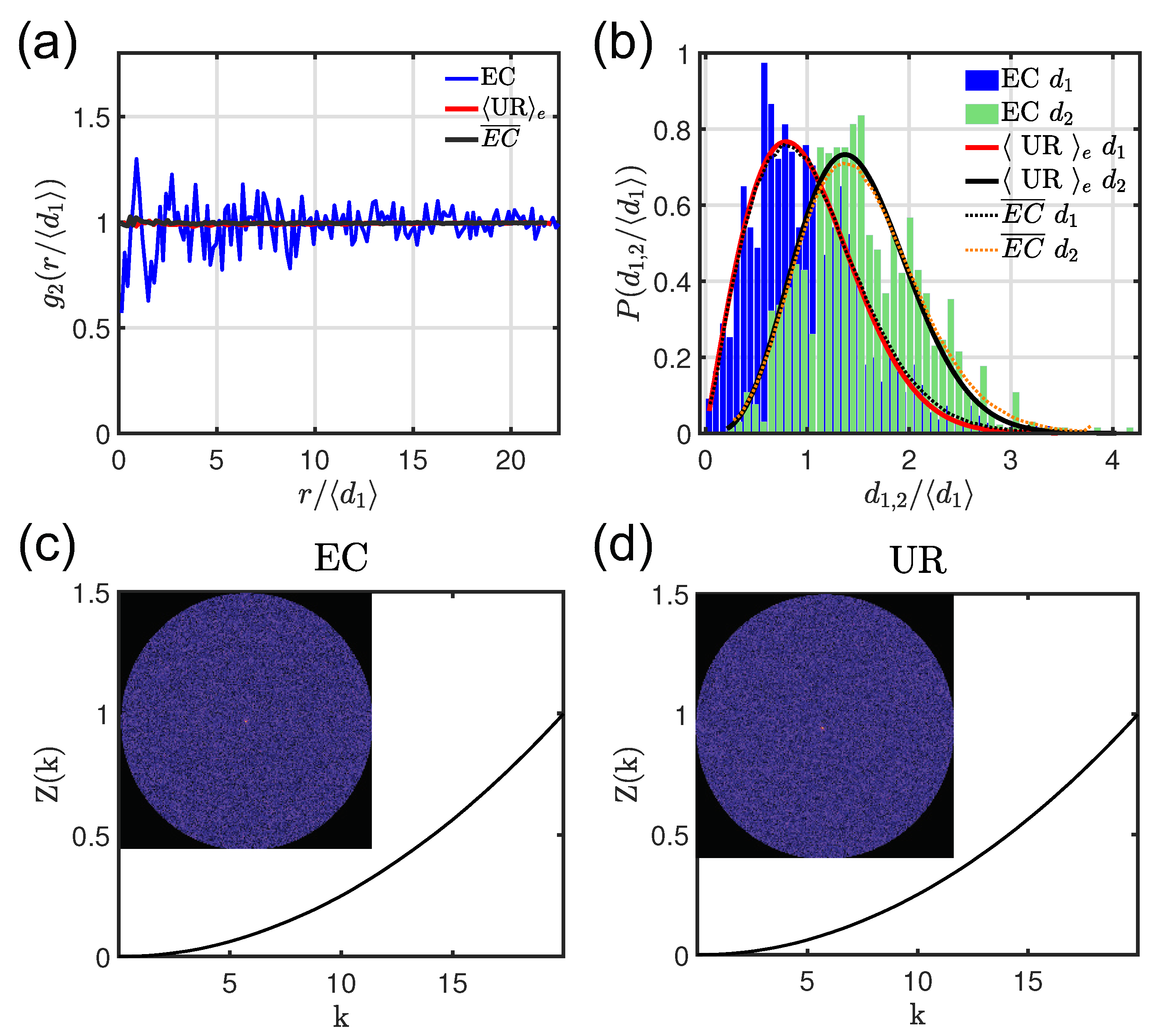
In order to obtain quantitative information on the degree of local structural order of $EC$ and $EC$$DL$ point patterns, we have computed their radial distribution functions $g\left(r\right)$, which give the probability of finding two particles separated by a distance r [55]. In Figure 2a we display the $g\left(r\right)$ of the representative $EC$ point pattern shown in Figure 1b (blue line) and we compare it with the disorder-averaged $g\left(r\right)$ of a uniform random ($UR$) structure considering 200 realizations of disorder (red line). In order to systematically analyze the correlation properties of $EC$ structures, we have considered 900 different elliptic curves generated by a uniform sample of the integer parameters A and B in the range (1, 30). The arithmetic average value of the $g\left(r\right)$ for all the investigated $EC$ structures is shown by the black line in Figure 2a. This quantity clearly demonstrates the uncorrelated nature of $EC$ structures akin to the average behavior of Poisson random point patterns. To gain more information on the peculiar geometrical arrangements of the points compared to $UR$ systems we studied the probability density functions of the first ($P\left(d_1\right)$) and second ($P\left(d_2\right)$) neighbor distances [25,55]. The results of this analysis are presented in panel Figure 2b. The $P\left(d_1\right)$ and $P\left(d_2\right)$ functions can be analytically approximated using the following expression:

$$P\left(d_k\right)=\frac{2{\left(\xi \pi r^2\right)}^k}{r(k-1)!}exp(-\xi \pi r^2),$$

(3)

where $P\left(d_k\right)$ is probability density function for the k-neighbor particle spacing of homogeneous Poisson point patterns with intensity $\xi$ evaluated as $N/\pi R^2$. Here N is the number of points in the array, which varies between 1926 and 2106, and R is the maximum radial coordinate of the system [31,55]. We notice that while the $P\left(d_1\right)$ and $P\left(d_2\right)$ distributions for a single $EC$ array fluctuate significantly, their average over the 900 investigated $EC$ structures with different A and B parameters can be precisely fitted using the analytical expression in Equation (3).

Aperiodic deterministic structures are complex structures with varying degrees of order and spatial correlations ranging from quasicrystals to more disordered amorphous structures with diffuse spectra [25,56,57]. In order to characterize the structural order of $EC$ point patterns, we have analyzed their spatial Fourier spectra by evaluating the static structure factor as

$$S\left(k\right)=\frac{1}{N}\sum _{n=1}^N\sum _{m=1}^N{e}^{-i\mathbf{\text{k}}\dot{(}{\mathbf{\text{r}}}_n-{\mathbf{\text{r}}}_m)}$$

(4)

Interestingly, the inset of Figure 2c shows that $EC$ aperiodic structures are characterized by diffuse diffraction spectra that are typically associated to homogenuous and isotropically disordered media (see the inset of Figure 2d). In order to get more information on the nature of these spectra, we have analyzed the behavior of the integrated intensity function defined as [22]:

$$Z\left(q\right)={\int }_{-q}^q{\int }_{-q}^q\left|S(k_x,k_y)\right|d{k}_{x}d{k}_y$$

(5)

For two-dimensional (2D) arrays, this function characterizes the distribution of the diffracted intensity peaks contained within a square region, centered at the origin, with a maximum size of $2k\times 2k$ in the reciprocal space [43]. Interestingly, Equation (5) has also been recently used as a tool to quantitatively characterize the type of hyperuniformity of quasicrystalline point sets generated by projection method by studying its scaling behavior as k tends to zero [58,59]. We recall that any diffraction intensity pattern can be regarded as a spectral measure ${\mu }_d$ that, thanks to the well-known Lebesgue’s decomposition theorem [56,57,60], can be uniquely decomposed in term of three kinds of primitive spectral components, or a mixture of them. Specifically, any diffraction spectra measure can be expressed as ${\mu }_d={\mu }_p\cup {\mu }_{sc}\cup {\mu }_{ac}$, where ${\mu }_p$, ${\mu }_{sc}$ and ${\mu }_{ac}$ refer to the pure-point, singular continuous, and absolutely continuous spectral components, respectively [22,23,56]. In particular, in both periodic and quasiperiodic structures there are regions where $Z\left(q\right)$ is constant due to the pure point nature of the spectrum. Therefore, over spectral gap regions $Z\left(q\right)$ remains constant and presents jump discontinuities every time an isolated Bragg peak is integrated over. On the contrary, for structures with absolutely continuous Fourier spectra the integrated intensity function is continuous and differentiable. Finally, in the case of structures with singular-continuous spectra like the ones generated by the distribution of the prime number on complex quadratic fields and quaternion rings [43], the Bragg peaks are no longer well-separated but clustered into a hierarchy of self-similar contributions giving rise to a weak continuous component in the spectrum that smoothly increases the value of $Z\left(q\right)$ in between consecutive plateaus. In Figure 2c,d we report the calculated $Z\left(q\right)$ for $EC$ and $UR$ configurations, respectively. The results did not show any appreciable difference compared to $UR$ systems, indicating that elliptic curves are structures characterized by an absolutely continuous diffraction spectral measure.

We now investigate the scattering spectra and wave localization properties of the elliptic curves defined over the finite field ${\mathbb{F}}_{2111}$ by using the Green’s matrix method. This formalism allows for a full description of open three-dimensional (3D) scattering resonances of large-scale structures at a relatively low computational cost if compared to traditional numerical methods such as finite difference time domain (FDTD) or finite element method (FEM) techniques [25,31,61]. Moreover, this approach provides access to all the scattering resonances of a system composed of vector electric dipoles in vacuum and accounts for all the multiple scattering orders. The point-scatterer assumption implies that the scatterer size must be much smaller than the wavelength. Specifically, in this limit each scatterer is described by a Breit–Wigner resonance at frequency ${\omega }_0$ and width ${\mathsf{\Gamma }}_0$ (${\mathsf{\Gamma }}_0\ll {\omega }_0$). The scattering resonances or quasi-modes of an array can be identified with the eigenvectors of the Green’s matrix $\overleftrightarrow{G}$ which, for N vector dipoles, is a $3N\times 3N$ matrix with components [20]:

$$G_{ij}=i\left({\delta }_{ij}+{\tilde{G}}_{ij}\right)$$

(6)

${\tilde{G}}_{ij}$ has the form:

$${\tilde{G}}_{ij}=\frac{3}{2}\left(1-{\delta }_{ij}\right)\frac{e^{i{k}_0{r}_{ij}}}{i{k}_0{r}_{ij}}\left\{\left[\mathit{U}-{\widehat{\mathit{r}}}_{ij}{\widehat{\mathit{r}}}_{ij}\right]-\left(\mathit{U}-3{\widehat{\mathit{r}}}_{ij}{\widehat{\mathit{r}}}_{ij}\right)\left[\frac{1}{{\left(k_0{r}_{ij}\right)}^2}+\frac{1}{i{k}_0{r}_{ij}}\right]\right\},$$

(7)

when $i\ne j$ and 0 for $i=j$, and where $k_0$ is the wavevector of light, the integer indexes $i,j\in 1,\cdots ,N$ refer to different particles, $\mathit{U}$ is the 3 × 3 identity matrix, ${\widehat{\mathit{r}}}_{ij}$ is the unit vector position from the i-th and j-th scatter while $r_{ij}$ identifies its magnitude. This method is an excellent tool to study light scattered by atomic clouds but also provides fundamental insights into the physics of periodic, aperiodic, and uniform random systems of small and sufficiently well-separated scattering particles [4,20,21,25,31,43,61,62,63,64,65,66,67,68]. The Green’s matrix (6) is a non-Hermitian matrix. As a consequence, it has complex eigenvalues ${\mathsf{\Lambda }}_n$ ($n\in 1,2,\cdots ,3N$) with $\mathsf{\Im }\left[{\mathsf{\Lambda }}_n\right]=({\omega }_0-{\omega }_n)/{\mathsf{\Gamma }}_0$ and $\mathsf{\Re }\left[{\mathsf{\Lambda }}_n\right]={\mathsf{\Gamma }}_n/{\mathsf{\Gamma }}_0$ [20,65,66,67,68]. Moreover, it is important to realize that the Green’s matrix method is an eigenvalue method that captures the fundamental physics of multiple scattering of vector waves for any assembly of electric scattering point dipoles. In addition, this powerful method enables a clear separation between the geometry of the scattering arrays (the arrangement of the dipoles) and the material properties and sizes of the individual particles that are captured by a retarded polarizability or by the refractive index. As a result, the predictions of the Green’s approach should be considered “universal” in the limit of electric dipole scatterers, meaning that the size and the refractive index of the particles can be taken into account after the diagonalization of the Green’s matrix by extracting the frequency ${\omega }_0$ and ${\mathsf{\Gamma }}_0$ from the central position and the lineshape of the scattering cross section (computed using for example the Mie–Lorentz theory in the dipole limit) of a single particle.

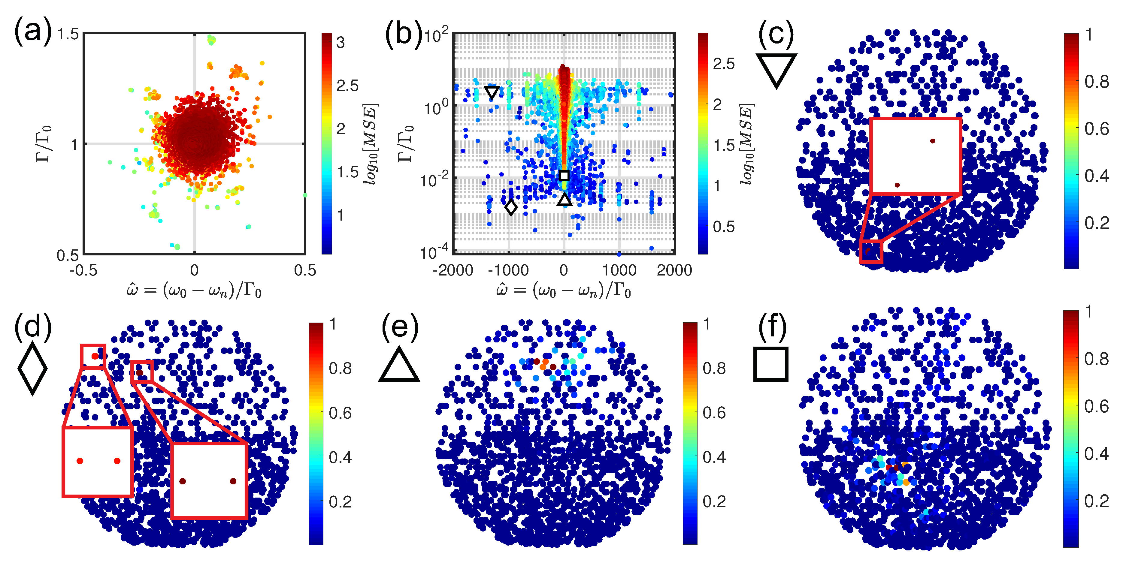
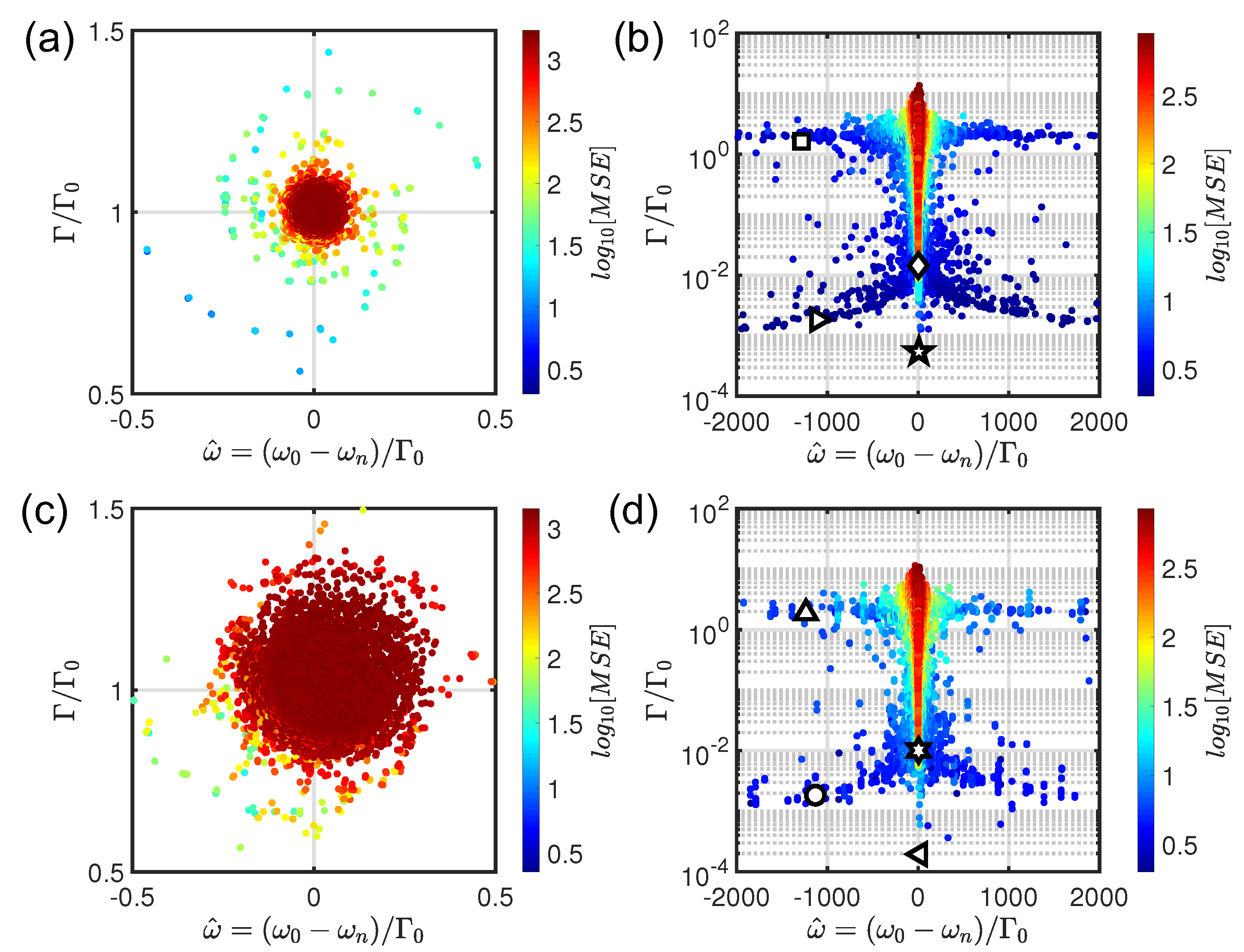
We have applied this formalism to both $UR$ and $EC$ arrays and studied the light scattering properties in the plane of these arrays by analyzing the behavior of their scattering resonances embedded in 3D. In order to do that, we have diagonalized numerically the $3N\times 3N$ Green’s matrix (7). The distribution of the resonant complex poles ${\mathsf{\Lambda }}_n$, color coded according to the ${log}_{10}$ values of the modal spatial extent (MSE), is reported in Figure 3a,b for the $UR$ and in Figure 3c,d for the representative $EC$ configuration shown in Figure 1b, respectively. Specifically, panels (a,c) and panels (b,d) refer to low and high optical density $\rho {\lambda }^2$, respectively. Here $\rho$ is the number of particles per unit area while $\lambda$ is the optical wavelength and $\rho {\lambda }^2$ is a measure of the scattering strength of the systems. Instead, the MSE parameter characterizes the spatial extent of a photonic mode [69]. It is important to emphasize that the dimensionality of the studied electromagnetic problem is 3D, but the electromagnetic field of a scattering resonance is not only spatially confined in the plane of the array but it also leaks out from such a plane with a characteristic time proportional to its quality factor [31].

At low optical density ($\rho {\lambda }^2=0.01$), the distribution of the complex poles of $N=1630$ electric point dipoles randomly located inside a circular region is highly uniform and is characterized by a circular shape with distinctive spiral arms that are weakened when the electric dipoles are arranged in $EC$ geometries (see Figure 3c). These spectral regions are typically populated by scattering resonances localized over small clusters of scatterers, down to only two particles [21,67]. The subradiant dark states, also called proximity resonances, are characterized by MSE = 2 [67,70] (see also Figure 4a,b). Interestingly, the absence of these scattering resonances in a class of aperiodic spirals, called Vogel spirals, was recently connected to the ability of these structures to localize vector waves thanks to their peculiar correlation properties [31].

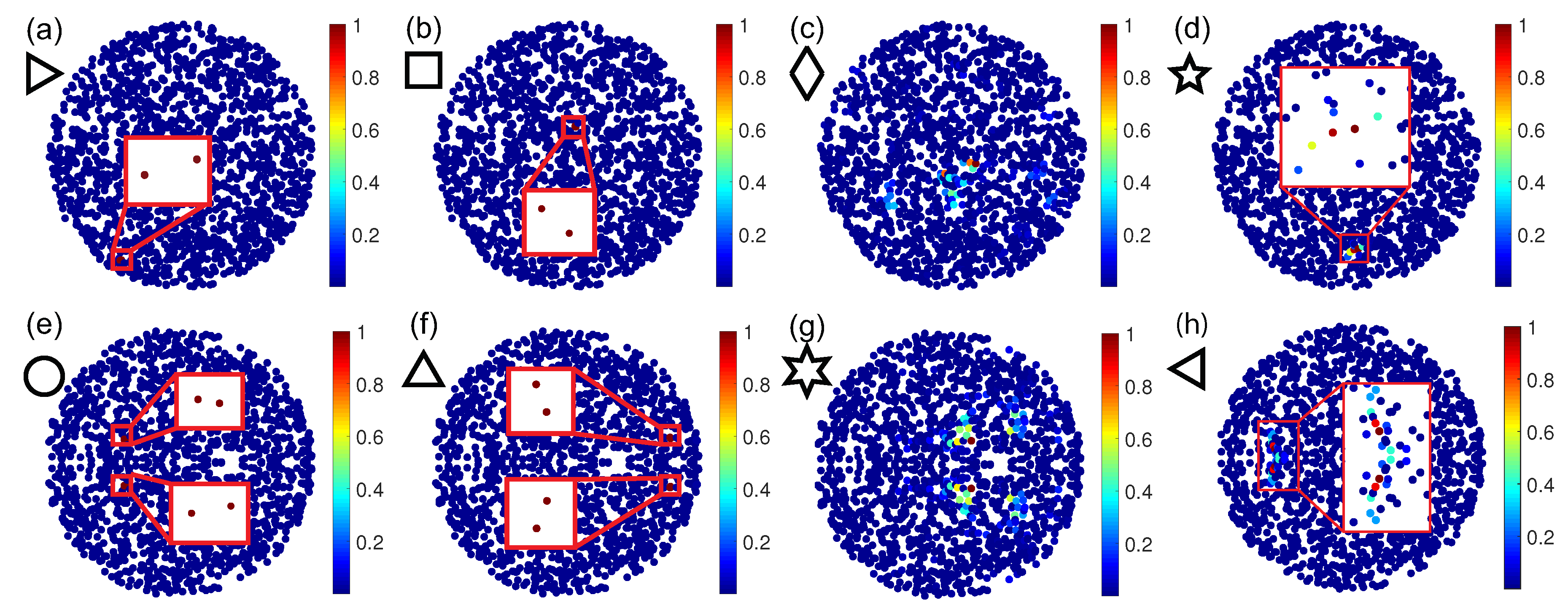
In order to understand the nature of the scattering resonances that characterize EC-based structures in the strong scattering regime ($\rho {\lambda }^2=50$), we have analyzed the spatial distributions of a few representative optical modes identified by the symbols shown in Figure 3b,d. Figure 4 shows a survey of representative spatial distribution of the Green’s eigenvectors for $UR$ (panels (a–d)) and $EC$ geometries (panels (e–h)), respectively. From the complex eigenvalues distribution and from the selected spatial field profiles, we can clearly distinguish among three different types of scattering resonances. Let us start by analyzing the $UR$ configuration. The first type of scattering resonances correspond to short-lived quasi-modes (${\mathsf{\Gamma }}_n/{\mathsf{\Gamma }}_0>1$) that are delocalized across the all arrays ($MSE\sim N$). Moreover, this spectral region is also populated by proximity resonances, as shown in Figure 4b. This is a clear signature of the fact that proximity resonances are not related to interference-driven light localization because they do not require multiple scattering in order to occur [25,31,67,70]. Finally, there are resonances that populate the dispersion branch around $\widehat{\omega }=-1$ with $\mathsf{\Gamma }/{\mathsf{\Gamma }}_0<{10}^{-1}$. These quasi-modes are long-lived resonances with $\mathsf{\Gamma }/{\mathsf{\Gamma }}_0$ in the range $[{10}^{-2},{10}^{-1}]$ extended over almost all the particles (see Figure 4c) or clustered over few particles near the array boundaries (see also the discussion of Figure 6a for more details). However, even if the main characteristics of the complex eigenvalues distribution of $EC$ structures is very similar to the $UR$ ones, a deeper analysis unveils important differences. First of all, strictly speaking $EC$ structures do not show traditional proximity resonances but clustered quasi-modes ($MSE\ge 4$) associated to the structural mirror symmetry along the x-axis, as shown in Figure 4e,f. Another important difference arises when looking at the dispersion branch around $\widehat{\omega }=-1$. Indeed, the $EC$-based arrays feature longer-lived and clustered resonances (${\mathsf{\Gamma }}_n/{\mathsf{\Gamma }}_0\sim {10}^{-4}$ with $MSE\ge$ 12) compared to standard $UR$ structures, see Figure 4h. These more extended, long-lived resonances are similar to the critical scattering resonances that are typical of fractal and multifractal systems. These optical modes characterized by a power-law envelope localization and multifractal field intensity oscillations [25,26,33,39,43,71].

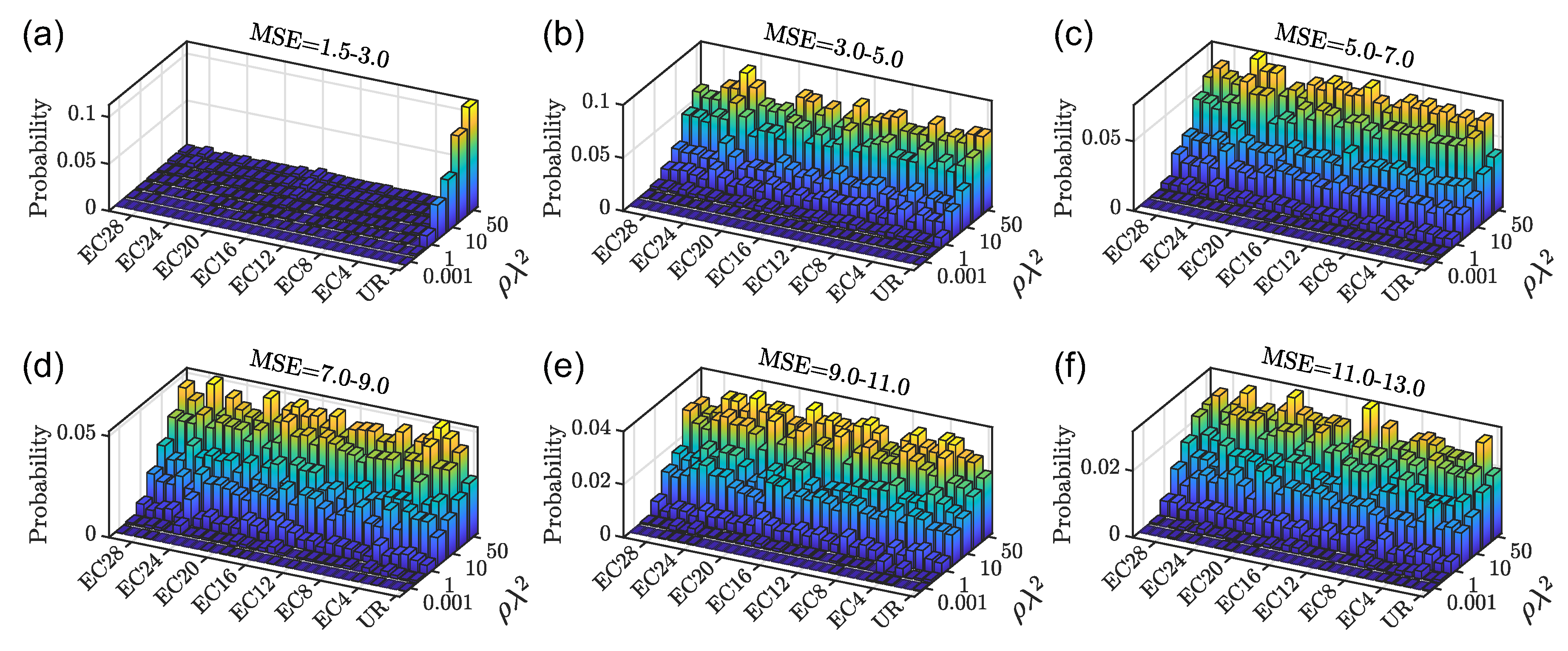
To gain additional insights on the nature of the scattering resonances of $EC$-based arrays compared to $UR$ systems, we have evaluated the proportion of modes that extend over a number of particles specified by the range of the MSE values considered. In particular, we computed the probability of the number of scattering resonances in different MSE ranges and at different optical densities. Figure 5 shows the results of this study. First of all, Figure 5a indicates that for $EC$ point patterns the probability of obtaining resonances localized over at most three scatterers is negligible compared to UR structures, shown in the first column of Figure 5. This is regardless of the value of the optical density. In contrast, proximity resonances do appear in UR systems even at low optical density ($\rho {\lambda }^2\ge 1$). By increasing the $MSE$ threshold, the probability of finding scattering resonances localized over large clusters of particles is always larger for the analyzed $EC$ configurations compared to the UR reference structures. Therefore, our analysis provides evidence that, differently from the case of uniform random systems, the mechanism of localization in EC-based structures proceeds through wave tunneling and trapping over few-particle clusters via the formation of Efimov-like resonances [72].

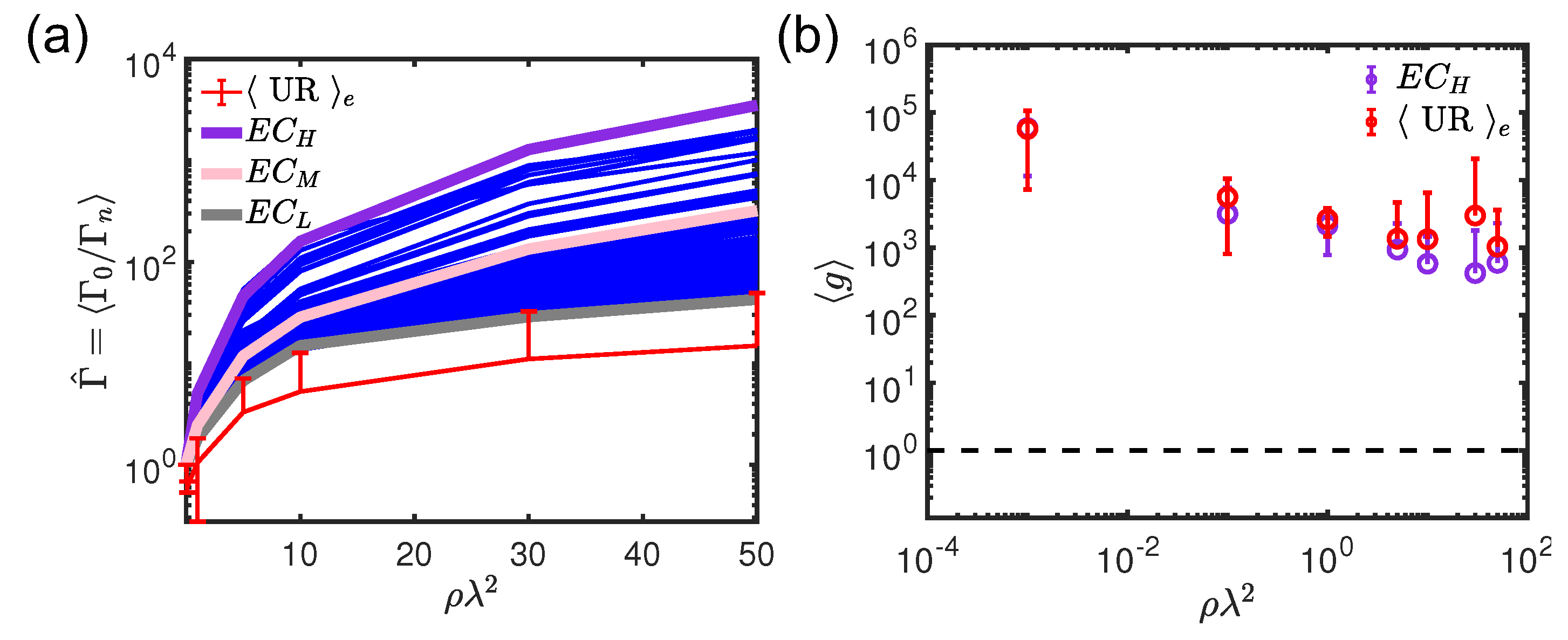
In order to analyze the light localization behavior, we have evaluated the modal average lifetime [31,62,63], the Thouless conductance g, also called Thouless number [73,74,75], and the level spacing distribution [76,77]. The average modal lifetime, defined as $\widehat{\mathsf{\Gamma }}=\langle {\mathsf{\Gamma }}_0/{\mathsf{\Gamma }}_n\rangle$, provides the mean-time that light spends inside a medium [31,62,63]. Figure 6a compares the averaged modal lifetime of the 900 different elliptic curves over ${\mathbb{F}}_{2111}$ with respect to the value of $\widehat{\mathsf{\Gamma }}$ produced by 10 different realizations of $UR$ structures. Interestingly, all the $EC$ structures show a larger average modal lifetime for all the analyzed $\rho {\lambda }^2$ values demonstrating enhanced light-matter interaction compared to random uniform random systems. The ability to confine and eventually localized light is also described by the Thouless conductance, which is a parameter that characterizes the degree of spectral overlap between different optical scattering resonances. In order to demonstrate light localization, the Thouless conductance, which is proportional to the scattering mean free path, must decrease below the value 1 when increasing the scattering strength, i.e., increasing the optical density $\rho {\lambda }^2$. Within the Green’s matrix formalism, it is defined as the ratio of the dimensionless lifetime ${\left(\delta \omega \right)}^{-1}=1/\mathsf{\Im }\left[{\mathsf{\Lambda }}_n\right]$ to the spacing of nearest dimensionless resonance frequencies $\delta \omega =\mathsf{\Re }\left[{\mathsf{\Lambda }}_n\right]-\mathsf{\Re }\left[{\mathsf{\Lambda }}_{n-1}\right]$ [20]:

$$\langle g\rangle =\frac{\overline{\delta \omega }}{\overline{\Delta \omega }}=\frac{{\left(\overline{1/\mathsf{\Im }\left[{\mathsf{\Lambda }}_n\right]}\right)}^{-1}}{\overline{\mathsf{\Re }\left[{\mathsf{\Lambda }}_n\right]-\mathsf{\Re }\left[{\mathsf{\Lambda }}_{n-1}\right]}}$$

(8)

where $\overline{\{\cdots \}}$ indicates the average of g over a frequency interval of width 2${\mathsf{\Gamma }}_0$ centered in ${\omega }_0$. This frequency stripe selection is necessary due to the strong frequency dependence of the light localization behavior [31]. On the other hand, averaging over all scattering frequencies will produce biased results due to the mixing of different types of light regimes [75]. Differently from the uniform random media, we do not need to consider any ensemble averages because the $EC$ structures are deterministic. Figure 6b compares the semilog plot of the Thouless conductance, as a function of $\rho {\lambda }^2$, obtained by using Equation (8) after diagonalizing the $3N\times 3N$ Green’s matrix of the $EC$ structure with the highest $\widehat{\mathsf{\Gamma }}$ (violet line in Figure 6a) with respect to the uniform random scenario. Even though $EC$ structures are characterized by longer-lived critical resonances than $UR$ systems, the $\langle g\rangle$ parameter clearly indicates that the light localization transition is never achieved, since $\langle g\rangle$ is always larger than 1. This is due to two factors: the presence of degenerate proximity resonances (like the ones shown in Figure 4e,f) and the absence of any structural correlations. The absence of structural correlations was recently identified as the factor preventing light localization to occur in uniform random arrays when the vector nature of light is taken into account [20,31,66].

In order to further investigate the spectral properties of $EC$ arrays we considered the distribution of level spacing $P\left(s\right)$ that provides important information about the electromagnetic propagation for both closed- and open-scattering systems [25]. Indeed, the shape of $P\left(s\right)$ depends on the spatial extent of the system eigenmodes. In particular, for open weakly disordered random media the probability density function of spacings between nearest eigenvalues ${\mathsf{\Lambda }}_i$ and ${\mathsf{\Lambda }}_{i+1}$ is described by:

$$P\left(s\right)=\frac{3^4{\pi }^2}{2^7}{s}^{3}exp\left(-\frac{3^2\pi }{2^4}{s}^2\right),$$

(9)

where $s=|\Delta \mathsf{\Lambda }/\langle |\Delta \mathsf{\Lambda }|\rangle |$ is the normalized eigenvalue spacing [66,76,77]. The important feature of this equation is the so-called level-repulsion phenomenon: $P\left(s\right)\to 0$ when $s\to 0$. The level repulsion is a characteristic of extended/delocalized scattering resonances that repel each other in the complex plane [25,66]. On the contrary, the appearance of localized states leads to a suppression of the eigenvalue repulsion because two spatially localized states hardly influence each other when strongly localized in different parts of the medium. Consequently, distinct modes with infinitely close energies are allowed and the distribution of level spacings is described in this more localized regime by the Poisson distribution:

$$P\left(s\right)\approx exp(-s)$$

(10)

Notably, the level spacing statistics is very well described by Equation (10) in the strong scattering regime for closed as well as for open (dissipative) systems [25,76].

However, the level statistics of deterministic aperiodic systems displays different features with respect to the uniform random scenario. In our previous works, we have investigated the transition from the presence to the absence of level repulsion by increasing $\rho {\lambda }^2$ in different open, deterministic, and aperiodic planar systems [25,31,43]. We have found that the distribution obeys at $\rho {\lambda }^2$ < 1 the critical cumulative probability density:

$$I\left(s\right)=exp[\mu -\sqrt{{\mu }^2+{\left(A_{c}s\right)}^2}],$$

(11)

where $\mu$ and $A_c$ are fitting parameters. This is attributed to the formation of a large number of critical scattering resonances. Indeed, Equation (11) was successfully applied to describe the energy level spacing distribution of an Anderson Hamiltonian containing ${10}^6$ lattice sites at the critical disorder value, i.e., at the metal–insulator threshold where it is known that all the wave functions exhibit multifractal scaling properties [46]. We remark that the presence of a critical statistics in the spectral behavior of $EC$ structures occurs over a broad range of optical densities compared to the case of random media in which criticality is achieved only at the threshold density ${\rho }_c$ [25,31,43].

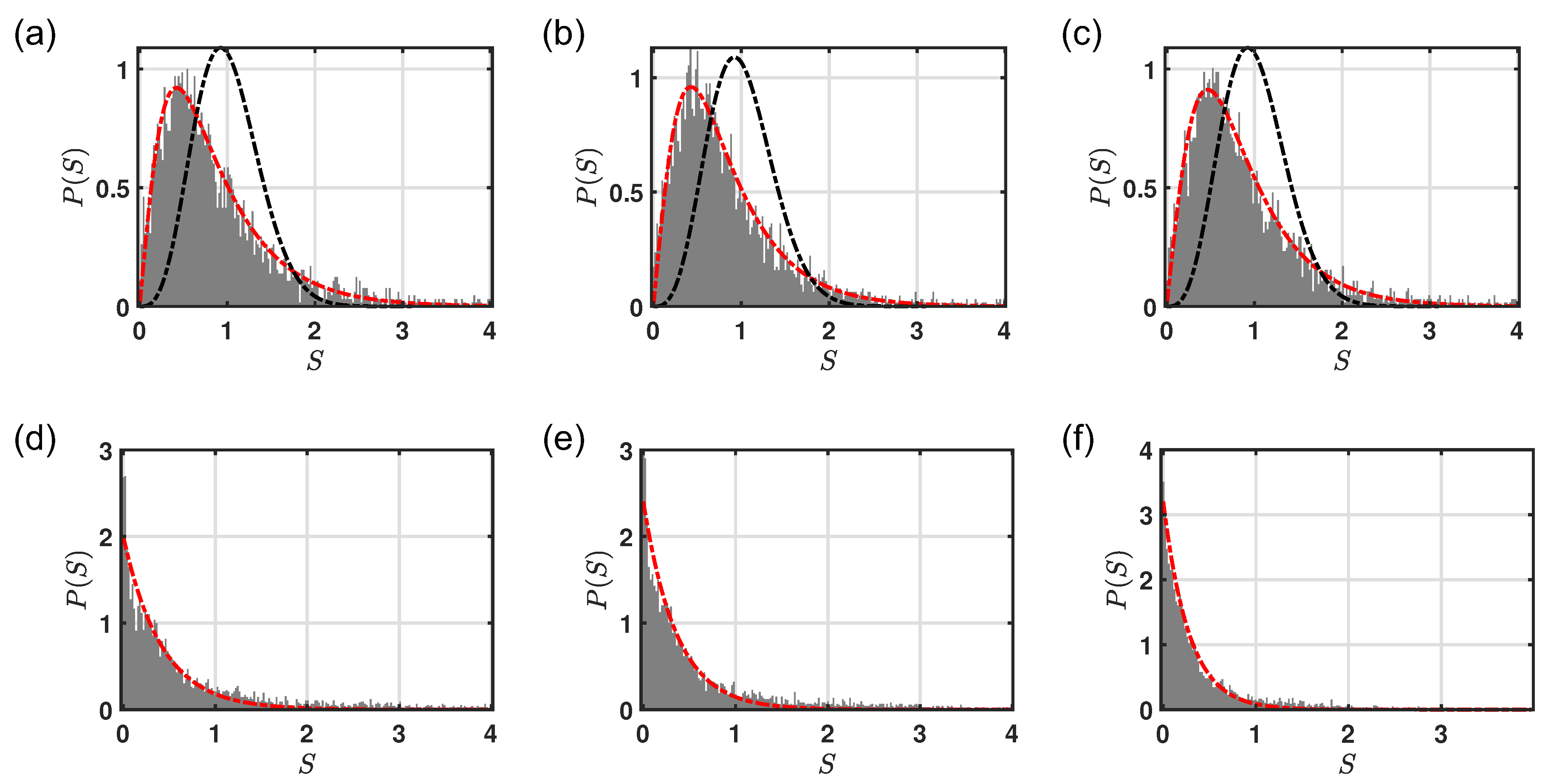
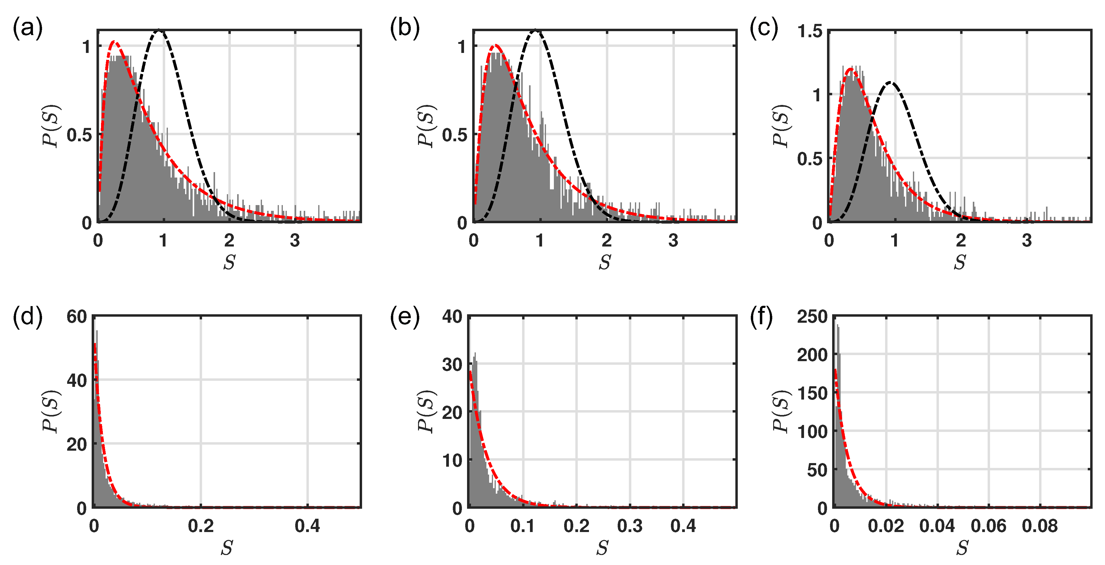
The results shown in Figure 7 demonstrate that the critical behavior is a generic attribute of all the investigated $EC$ structures. Indeed, panels (a,d), (b,e), (c,f) show a transition from the presence to the absence of level repulsion by increasing $\rho {\lambda }^2$ for the $E{C}_H$, $E{C}_M$, and $E{C}_L$ point patterns, defined in Figure 6a, respectively. At low optical density (panels (a–c)), the $P\left(s\right)$ of the $EC$ point patterns and $UR$ configurations are well described by, respectively, Equation (11) (dotted dashed red lines) and Equation (9) (dotted dashed black lines). On the other hand, $P\left(s\right)$ follows the Poisson distribution (10) for both $UR$ and $EC$ configurations for high optical density ($\rho {\lambda }^2=50$). Since the presence of a critical statistics is associated to the multifractal nature of the spectrum, the criticality discovered in $EC$ structures opens intriguing opportunities to engineer wave transport in these novel aperiodic systems [11,29].

We now address the structural and spectral properties of aperiodic point patterns obtained by the solution of the discrete logarithm problem, as discussed in Section 2. Figure 8 displays the main results of the structural analysis, based on the radial distribution function and on the first and second neighbor distributions. $EC$$DL$ structures, generated by the coordinate $(M_y;k)$, show higher degree of structural correlations than the $EC$$DL$ that are symmetric with respect to the x-axis, i.e., produced by the pairs $(M_x;k)$. However, after averaging over 72 different $EC$$DL$ arrays generated by randomly selecting the starting point W from the $E{C}_H$ and $E{C}_L$ point patterns (the elliptic curve configurations that show the highest and lowest modal lifetime, as reported in Figure 6a), the $g\left(r\right)$ becomes constant and very close to 1 in value, indicating absence of any structural correlations (see the black lines in Figure 8a,c). Moreover, also the averaged first (black dash dotted lines in Figure 8b,d) and second (orange dash dotted lines in Figure 8b,d) neighbor distributions are very similar to the analytical expression of Equation (3) valid for homogeneous Poisson point processes [55]. Therefore, we have found that on average also the $EC$$DL$ structures are spatially uncorrelated point patterns (incidentally, this property explains why the discrete logarithm problem on elliptic curve is a very hard problem). This behavior is also confirmed by analyzing their spectral properties via the diagonalization of the matrix (7). Indeed, the results of Figure 9 are very similar to the ones reported in Figure 3 for the EC structures. Specifically, the complex eigenvalues distribution of $EC$$DL$ point patterns at low optical density ($\rho {\lambda }^2=0.01$) shows the same characteristics of elliptic curves: a circular disk region as for the $UR$ structures but without the distinctive spiral arms populated by the proximity resonances (see Figure 9a). Instead, the distribution of the complex scattering poles at large optical density shows similar features in both $EC$$DL$ and $UR$ arrays. In particular, both proximity and clustered quasi-modes, with $MSE\ge 4$, are present. Proximity resonances populate mostly the spectral region with ${\mathsf{\Gamma }}_n>{\mathsf{\Gamma }}_0$, while these clustered optical modes characterize the sub-radiant spiral arms (see Figure 9c,d). Moreover, the dispersion branch around $\widehat{\omega }=-1$ is characterized by both scattering resonances clustered on few particles near the array boundaries, similar to the $UR$ scenario, and by critical quasi-modes, as shown in Figure 9e,f, respectively. Indeed, a clear spectral region characterized by longer-lived modes with large value of $MSE$ is clearly visible is Figure 9b when $\widehat{\omega }=-1$ and $\mathsf{\Gamma }/{\mathsf{\Gamma }}_0<{10}^{-1}$.

In order to understand how critical quasi-modes influence the light-matter interaction properties of $EC$$DL$ geometry, we have also evaluated their probability density function by selecting different $MSE$ ranges. We discovered that the probability of finding scattering resonances localized over a clusters of scatterers is always larger than in the $UR$ scenario (see Figure 10). Of particular interest is the situation depicted in Figure 10a where the $MSE$ range is fixed between 1.5 and 3, i.e., the resonances are localized over at most 3 particles. Whereas $EC$ point patterns are always characterized by the absence of proximity resonances, $EC$$DL$ structures instead show the presence of long-lived, strongly localized sub-radiant states even for the lowest $MSE$ range considered. Specifically, we observed that proximity resonances are always present in the type of $EC$$DL$ point patterns that lack reflection symmetry, discussed in Section 2. Moreover, the modal average lifetime (Figure 11a), the Thouless conductance (Figure 11b), and the level spacing statistics (Figure 12) clearly demonstrate the role played by the critical scattering resonances also for the case of $EC$$DL$ structures. However, we found that the average modal lifetime of 36 $EC$$DL$ aperiodic structures is always larger than the $UR$ scenario. Moreover, the Thouless conductance of the $EC$$DL$ and $EC$ structures with the largest $\widehat{\mathsf{\Gamma }}$ (orange and violet line in Figure 6a and Figure 11a, respectively) are comparable and both larger than what can be achieved in $UR$ systems, demonstrating the potential to obtain stronger light-matter interaction in these novel aperiodic arrays.

4. Light Scattering Properties and the Extended Green’s Matrix Method

As discussed in the previous section, the Green’s matrix spectral method is an excellent approximation to study light scattering by atomic clouds and can give fundamental insights into the physics of multiple scattered light by small particles within the dipole approximation. However, this method is an oversimplification in the case of realistic scatterers that are, instead, characterized by higher-order multipolar resonances. The number of these peaks depends by the scatterer material and by the size parameter x defined as $kR$, where k is the wavelength number, while R is the scatterer radius. Specifically, light scattering by a homogeneous, isotropic and spherical particle with radius R illuminated by a linearly polarized plane wave traveling in the z-direction $\mathit{k}=[0;0;k]=[0;0;\omega /c]$ can be calculated by using the Mie–Lorentz theory [78]. If the size of scatterers in an array is smaller than the incident wavelength and they are far enough from each others, the light scattering problem can be described by using only the dipolar term in the general multipolar expansion [79]. However, the interplay between the electric and magnetic dipolar responses of small particles is a key ingredient in determining their directional scattering features. Therefore, in order to obtain a more realistic description of light scattering from these complex arrays we must go beyond the simple electric dipole framework. For this reason, we provide an extension of the Green’s matrix method that takes into account both the first-order Mie–Lorentz coefficients, referred to as the electric and magnetic coupled dipole approximation (EMCDA) [78,80]. In this approximation, each particle is characterized by two dipoles (electric dipole (ED) and magnetic dipole (MD)) corresponding to the induced electric and a magnetic polarizability [81].

In order to derive rigorously the EMCDA approximation, we must start from the electric ${\mathit{E}}_p$ and magnetic fields ${\mathit{H}}_p$ at a distance r and direction $\mathit{n}$ produced by an electric dipole $\mathit{p}$. In the cgs unit system, we have [82]:

$$\begin{array}{c}\hfill \begin{array}{c}{\mathit{E}}_p=\left[\mathit{p}\frac{e^{ikr}}{r}\left(k^2-\frac{1}{r^2}+\frac{ik}{r}\right)+\mathit{n}(\mathit{n}·\mathit{p})\frac{e^{ikr}}{r}\left(-k^2+\frac{3}{r^2}-\frac{3ik}{r}\right)\right]\hfill \\ {\mathit{H}}_p=\left[(\mathit{n}\times \mathit{p})\frac{e^{ikr}}{r}\left(k^2+\frac{ik}{r}\right)\right].\hfill \end{array}\end{array}$$

(12)

Equivalently, the field ${\mathit{E}}_m$ and ${\mathit{H}}_m$ produced by a magnetic dipole $\mathit{m}$ are give by [82]

$$\begin{array}{c}\hfill \begin{array}{c}{\mathit{E}}_m=-(\mathit{n}\times \mathit{m})\frac{e^{ikr}}{r}\left(k^2+\frac{ik}{r}\right)\hfill \\ {\mathit{H}}_m=\left[\mathit{m}\frac{e^{ikr}}{r}\left(k^2-\frac{1}{r^2}+\frac{ik}{r}\right)+\mathit{n}(\mathit{n}·\mathit{m})\frac{e^{ikr}}{r}\left(-k^2+\frac{3}{r^2}-\frac{3ik}{r}\right)\right].\hfill \end{array}\end{array}$$

(13)

By introducing the coefficients a, b, and d defined as [78,80]

$$\begin{array}{c}\hfill a=\frac{e^{i{k}_{0}r}}{r}{k}_0^2\left(1-\frac{1}{k_0^2{r}^2}-\frac{1}{i{k}_{0}r}\right)\end{array}$$

(14)

$$\begin{array}{c}\hfill b=\frac{e^{i{k}_{0}r}}{r}{k}_0^2\left(-1+\frac{3}{k_0^2{r}^2}+\frac{3}{i{k}_{0}r}\right)\end{array}$$

(15)

$$\begin{array}{c}\hfill d=\frac{e^{i{k}_{0}r}}{r}{k}_0^2\left(1-\frac{1}{i{k}_{0}r}\right)\end{array}.$$

(16)

We can rewrite Equations (12) and (13) in a shorter notation:

$$\begin{array}{c}\hfill \begin{array}{c}{\mathit{E}}_p=\mathit{p}a+\mathit{n}(\mathit{n}·\mathit{p})b\hfill \\ {\mathit{H}}_p=(\mathit{n}\times \mathit{p})d\hfill \\ {\mathit{E}}_m=-(\mathit{n}\times \mathit{m})d\hfill \\ {\mathit{H}}_m=\left[\mathit{m}a+\mathit{n}(\mathit{n}·\mathit{m})b\right]\hfill \end{array}.\end{array}$$

(17)

As a first step, our goal is to evaluate the total electric and magnetic fields at the ith particle (${\mathit{E}}_i$ and ${\mathit{H}}_i$) resulting from the electric and magnetic dipole moments of the jth particle. Explicitly, we can write, by using Equation (17), ${\mathit{E}}_i$ and ${\mathit{H}}_i$ as:

$$\begin{array}{c}\hfill {\mathit{E}}_i={\mathit{E}}_p^j+{\mathit{E}}_m^j=\left[a_{ij}{\mathit{p}}_j+b_{ij}({\mathit{n}}_{ij}·{\mathit{p}}_j){\mathit{n}}_{ij}\right]-d_{ij}({\mathit{n}}_{ij}\times {\mathit{m}}_j)\\ \hfill {\mathit{H}}_i={\mathit{H}}_p^j+{\mathit{H}}_m^j=d_{ij}({\mathit{n}}_{ij}\times {\mathit{p}}_j)+[a_{ij}{\mathit{m}}_j+b_{ij}({\mathit{n}}_{ij}·{\mathit{m}}_j){\mathit{n}}_{ij}],\end{array}$$

(18)

where the electric and magnetic dipole moments at the jth particle position are defined as ${\mathit{p}}_j={\alpha }_E{\mathit{E}}_j$ and ${\mathit{m}}_j={\alpha }_H{\mathit{H}}_j$, respectively [83]. The electric and magnetic polarizabilities ${\alpha }_E$ and ${\alpha }_M$ (that have units of a volume) are related to the first order Mie–Lorentz coefficients $a_1$ and $b_1$ as [81,84]:

$$\begin{array}{c}\hfill \begin{array}{c}{\alpha }_E=\frac{3\pi i}{2k_0^3}{a}_1\hfill \\ {\alpha }_H=\frac{3\pi i}{2k_0^3}{b}_1\hfill \end{array}.\end{array}$$

(19)

Here, $k_0$ is the wavenumber of the background medium, while $a_1$ and $b_1$ are derived from the equation

$$\begin{array}{c}\hfill \begin{array}{c}{a}_{\nu }=\frac{n{\psi }_{\nu }\left(nkR\right){\psi }_{\nu }^{\prime }\left(kR\right)-{\psi }_{\nu }\left(kR\right){\psi }_{\nu }^{\prime }\left(nkR\right)}{n{\psi }_{\nu }\left(nkR\right){\xi }_{\nu }^{\prime }\left(kR\right)-{\xi }_{\nu }\left(kR\right){\psi }_{\nu }^{\prime }\left(nkR\right)}\hfill \\ b_{\nu }=\frac{{\psi }_{\nu }\left(nkR\right){\psi }_{\nu }^{\prime }\left(kR\right)-n{\psi }_{\nu }\left(kR\right){\psi }_{\nu }^{\prime }\left(nkR\right)}{{\psi }_{\nu }\left(nkR\right){\xi }_{\nu }^{\prime }\left(kR\right)-n{\xi }_{\nu }\left(kR\right){\psi }_{\nu }^{\prime }\left(nkR\right)},\hfill \end{array}\end{array}$$

(20)

where R is the radius of the spherical scatterer, and n is the relative refractive index of the nanosphere with respect to the background medium. ${\psi }_{\nu }\left(x\right)$ and ${\xi }_{\nu }\left(x\right)$ are the Riccati–Bessel functions constructed from spherical Bessel functions via ${\psi }_{\nu }\left(x\right)=x{j}_{\nu }\left(x\right)$ and ${\xi }_{\nu }\left(x\right)=x{h}_{\nu }^{\left(1\right)}\left(x\right)$. In addition, $j_{\nu }\left(x\right)$ is the spherical Bessel function of the first type, and $h_{\nu }^{\left(1\right)}\left(x\right)$ is the spherical Hankel function of the first type. By substituting the dipole moments expressions into Equation (18), we finally obtain the total electric and magnetic fields at the i-th particle in the form:

$${\mathbf{E}}_i=a_{ij}{\alpha }_E{\mathbf{E}}_j+b_{ij}{\alpha }_E({\mathbf{E}}_j·{\mathbf{n}}_{ji}){\mathbf{n}}_{ji}-d_{ij}{\alpha }_H({\mathbf{n}}_{ji}\times {\mathbf{H}}_j)$$

(21)

$${\mathbf{H}}_i=a_{ij}{\alpha }_H{\mathbf{H}}_j+b_{ij}{\alpha }_H({\mathbf{H}}_j·{\mathbf{n}}_{ji}){\mathbf{n}}_{ji}+d_{ij}{\alpha }_E({\mathbf{n}}_{ji}\times {\mathbf{E}}_j).$$

(22)

To solve these coupled equations, it is convenient to express the various vector products in Equations (21) and (22) as matrix products [78,83]. In detail, by introducing the $3\times 3$ matrices $C_{ij}$ and $f_{ij}$, defined as:

$$C_{ij}=\left[\begin{array}{ccc}{a}_{ij}+b_{ij}{\left(n_{ij}^x\right)}^2& b_{ij}{n}_{ij}^x{n}_{ij}^y& b_{ij}{n}_{ij}^x{n}_{ij}^z\\ b_{ij}{n}_{ij}^y{n}_{ij}^x& a_{ij}+b_{ij}{\left(n_{ij}^y\right)}^2& b_{ij}{n}_{ij}^y{n}_{ij}^z\\ b_{ij}{n}_{ij}^z{n}_{ij}^x& b_{ij}{n}_{ij}^z{n}_{ij}^y& a_{ij}+b_{ij}{\left(n_{ij}^z\right)}^2\end{array}\right]$$

(23)

$$f_{ij}=\left[\begin{array}{ccc}0& -d_{ij}{n}_{ij}^z& d_{ij}{n}_{ij}^y\\ d_{ij}{n}_{ij}^z& 0& -d_{ij}{n}_{ij}^x\\ -d_{ij}{n}_{ij}^y& d_{ij}{n}_{ij}^x& 0\end{array}\right]$$

(24)

where $n_{ij}^{\beta }={\beta }_i-{\beta }_j$ ($\beta =x,y,$ and z) are the components of the direction vector from the jth to the ith particle, we can re-write Equations (21) and (22) in the compact form:

$$\left[\begin{array}{c}{\mathit{E}}_i\\ {\mathit{H}}_i\end{array}\right]=\left[\begin{array}{cc}{C}_{ij}& -f_{ij}\\ f_{ij}& C_{ij}\end{array}\right]\left[\begin{array}{cc}{\tilde{\alpha }}_E& 0\\ 0& {\tilde{\alpha }}_H\end{array}\right]\left[\begin{array}{c}{\mathit{E}}_j\\ {\mathit{H}}_j\end{array}\right],$$

(25)

where ${\tilde{\alpha }}_E$ and ${\tilde{\alpha }}_H$ are 3×3 diagonal matrices containing the polarizability ${\alpha }_E$ and ${\alpha }_H$ defined by Equation (19) in the case of isotropic materials.

Equation (25) defines the dyadic Green’s matrix ${\overleftrightarrow{G}}_{ij}$ that connects the electromagnetic field of the i-th-particle with the electromagnetic field of the j-th-particle. Specifically, ${\overleftrightarrow{G}}_{ij}$ is obtained as:

$${\overleftrightarrow{G}}_{ij}=\left[\begin{array}{cc}{C}_{ij}& -f_{ij}\\ f_{ij}& C_{ij}\end{array}\right]=\left[\begin{array}{cc}{\overleftrightarrow{G}}_{ij}^{ee}& {\overleftrightarrow{G}}_{ij}^{eh}\\ {\overleftrightarrow{G}}_{ij}^{he}& {\overleftrightarrow{G}}_{ij}^{hh}\end{array}\right].$$

(26)

The dyadic symbol $\overleftrightarrow{\{\cdots \}}$ is used to stress the fact that we are taking into account all the field components. Therefore, ${\overleftrightarrow{G}}_{ij}$ is a $6\times 6$ matrix. Moreover, one of the advantages of using cgs system unit is that the symmetry relations between electric and magnetic quantities are preserved, i.e., ${\overleftrightarrow{G}}^{ee}$ = ${\overleftrightarrow{G}}^{hh}$ and ${\overleftrightarrow{G}}^{eh}$ = $-{\overleftrightarrow{G}}^{he}$ [83].

The generalization of the formalism for N scatterers is straightforward. Equations (21) and (22) can be assembled using the a Foldy–Lax scheme such that the local fields at the position of the ith scatterer ${\mathit{E}}_i^{tot}$ and ${\mathit{H}}_i^{tot}$ are the sum of the scattered term of all the other particles plus the incident field (${\mathbf{E}}_{i,0}$; ${\mathbf{H}}_{i,0}$) on the ith particle

$$\begin{array}{cc}\hfill {\mathbf{E}}_i^{tot}& ={\mathbf{E}}_{i,0}+\sum _{j\ne i}^N{\alpha }_{E,i}{C}_{ij}{\mathbf{E}}_j-\sum _{j\ne i}^N{\alpha }_{H_i}{f}_{ij}{\mathbf{H}}_j={\mathbf{E}}_{i,0}+\sum _{j\ne i}^N\left[{\alpha }_{E,i}{\overleftrightarrow{G}}_{ij}^{ee}{\mathbf{E}}_j+{\alpha }_{H_i}{\overleftrightarrow{G}}_{ij}^{eh}{\mathbf{H}}_j\right]\hfill \end{array}$$

(27)

$$\begin{array}{c}\hfill {\mathbf{H}}_i^{tot}={\mathbf{H}}_{i,0}+\sum _{j\ne i}^N{\alpha }_{H,i}{\tilde{C}}_{ij}{\mathbf{H}}_j+\sum _{j\ne i}^N{\alpha }_{E,i}{\tilde{f}}_{ij}{\mathbf{E}}_j={\mathbf{H}}_{i,0}+\sum _{j\ne i}^N\left[{\alpha }_{H,i}{\overleftrightarrow{G}}_{ij}^{hh}{\mathbf{H}}_j+{\alpha }_{E_i}{\overleftrightarrow{G}}_{ij}^{he}{\mathbf{E}}_j\right].\end{array}$$

(28)

These last two equations can be rewritten as:

$$\mathsf{\Xi }\left(\mathit{r}\right)={\mathsf{\Xi }}_{inc}\left(\mathit{r}\right)+\mathit{M}\mathsf{\Xi }\left(\mathit{r}\right).$$

(29)

where $\mathsf{\Xi }$ is the vector containing the electric ${\mathit{E}}_i$ and magnetic field ${\mathit{H}}_i$, while $\mathit{M}$ is a linear integral operator describing the interactions between the scatterers. To solve Equation (29), successive approximations must be used. The first step is characterized by the Rayleigh–Gans–Debye (RGD) approximation [78,81]. Within this approximation, ${\mathsf{\Xi }}_{inc}\left(\mathit{r}\right)$ is equal to $\mathsf{\Xi }\left(\mathit{r}\right)$. In this way, we can compute the first-order estimation for every particles. After that, the iterative scheme is obtained by inserting the j-th interaction of the fields ${\mathsf{\Xi }}^j\left(\mathit{r}\right)$ into the right side of Equation (29) and evaluating the next interaction in the left side. The solution of Equation (29) is, therefore,

$$\mathsf{\Xi }\left(\mathit{r}\right)=\sum _{l=0}^{\infty }{\mathit{M}}^l{\mathsf{\Xi }}_{inc}\left(\mathit{r}\right),$$

(30)

which is a direct implementation of the well-know Neumann series

$${(\mathit{I}-\mathit{M})}^{-1}=\sum _{l=0}^{\infty }{\mathit{M}}^l$$

where $\mathit{I}$ is the unitary operator. A necessary and sufficient condition for the convergence of the Neumann-series is $∥M∥<1$. From a physical point of view, this iterative self consistent method lies in successive calculations of interactions between different scatterers. Therefore, the zero order level accounts for no interactions, the first approximation takes into account the influence of the scattering of each dipole on the others once, and so on.

It is very instructive to write down the compact matrix form of Equations (27) and (28) because it defines the full Green’s matrix $\overleftrightarrow{\check{G}}$. Explicitly, the full Green’s matrix has the form

$$\overleftrightarrow{\check{G}}=\left[\begin{array}{ccccc}\widehat{0}& {\overleftrightarrow{G}}_{12}& {\overleftrightarrow{G}}_{13}& \cdots & {\overleftrightarrow{G}}_{1N}\\ ⋮& \ddots & ⋮& ⋮& ⋮\\ {\overleftrightarrow{G}}_{j1}& \cdots & \widehat{0}& \cdots & {\overleftrightarrow{G}}_{jN}\\ ⋮& ⋮& ⋮& \ddots & ⋮\\ {\overleftrightarrow{G}}_{N1}& {\overleftrightarrow{G}}_{N2}& {\overleftrightarrow{G}}_{N3}& \cdots & \widehat{0}\end{array}\right],$$

(31)

where $\widehat{0}$ represents the $6\times 6$ zeros matrix, while the $6\times 6$ sub-block are expressed by the matrix (26). The $\overleftrightarrow{\check{G}}$ is a $6N\times 6N$ elements where N expresses the total number of scattereres.

Within this formalism, the extinction efficiency of a generic array of scattering particles can be directly obtained from the forward-scattering amplitude using the optical theorem for vector waves for both electric and magnetic polarizations, which results in [85]:

$$Q_{ext}=\frac{4\pi k_0}{\pi |E_{inc}{|}^{2}N{R}^2}\sum _{i=1}^N\mathsf{\Im }[\mathit{p}\left({\mathit{r}}_{\mathit{i}}\right)·{\mathit{E}}_{inc}^{*}\left({\mathit{r}}_i\right)+\mathit{m}\left({\mathit{r}}_i\right)·{\mathit{H}}_{inc}^{*}\left({\mathit{r}}_i\right)],$$

(32)

where $\mathit{p}\left({\mathit{r}}_i\right)={\alpha }_e\mathit{E}\left({\mathit{r}}_i\right)$, $\mathit{m}\left({\mathit{r}}_i\right)={\alpha }_m\mathit{H}\left({\mathit{r}}_i\right)$, R is the particle radius, N is the particle number, and the asterisk denotes the complex conjugate. Similarly, the absorption efficiency can be obtained by considering the energy dissipation of both dipoles in the system producing:

$$\begin{array}{cc}\hfill Q_{abs}=& \frac{4\pi k_0}{\pi |E_{inc}{|}^{2}N{R}^2}\sum _{i=1}^N{\left|\mathit{E}\left({\mathit{r}}_{\mathit{i}}\right)\right|}^2\left(\mathsf{\Im }\left[{\alpha }_e\left({\mathit{r}}_i\right)\right]-\frac{2}{3}{k}_0^3{\left|{\alpha }_e\left({\mathit{r}}_i\right)\right|}^2\right)\hfill \\ & +\frac{4\pi k_0}{|E_{inc}{|}^2}\sum _{i=1}^N{\left|\mathit{H}\left({\mathit{r}}_{\mathit{i}}\right)\right|}^2\left(\mathsf{\Im }\left[{\alpha }_m\left({\mathit{r}}_i\right)\right]-\frac{2}{3}{k}_0^3{\left|{\alpha }_m\left({\mathit{r}}_i\right)\right|}^2\right).\hfill \end{array}$$

(33)

The scattering efficiency can be always obtained by the difference of the extinction and the absorption efficiency, i.e., $Q_{sca}=Q_{ext}-Q_{abs}$. However, this operation requires high numerical accuracy in the computation of both $Q_{ext}$ and $Q_{abs}$ [83]. To avoid this problem it is possible to directly calculate the scattering efficiency $Q_{scat}$ by evaluating the power radiated in the far field by the oscillating electric and magnetic dipoles, which is [86]:

$$\begin{array}{cc}\hfill Q_{sca}& =\frac{k_0^4}{\pi |E_{inc}{|}^{2}N{R}^2}\int \left(\frac{d\sigma }{d\mathsf{\Omega }}\right)d\mathsf{\Omega }\hfill \\ & =\frac{k_0^4}{\pi |E_{inc}{|}^{2}N{R}^2}\int {\left|\sum _{i=1}^N{e}^{i{k}_0\mathit{n}·{\mathit{r}}_i}\{\mathit{p}\left({\mathit{r}}_i\right)-[\widehat{\mathit{n}}·\mathit{p}\left({\mathit{r}}_i\right)]\widehat{\mathit{n}}-\widehat{\mathit{n}}\times \mathit{m}\left({\mathit{r}}_{\mathit{i}}\right)\right|}^{2}d\mathsf{\Omega },\hfill \end{array}$$

(34)

where $\widehat{\mathit{n}}$ is an unit vector in the direction of scattering. Moreover, Equation (34) defines the differential scattering efficiency in the backward and forward direction when $\widehat{\mathit{n}}$ is equal to the tern $(0,0,-1)$ and $(0,0,1)$, respectively, if the excitation is assumed along the z-axis. Explicitly, the forward and backward scattering efficiencies are defined as:

$$\begin{array}{cc}\hfill \left(\frac{d\sigma }{d\mathsf{\Omega }}\right){|}_{\theta =0}& ={\left.\frac{4k_0^4}{|E_{inc}{|}^{2}N{R}^2}\frac{d\sigma }{d\mathsf{\Omega }}\right|}_{\theta =0}\hfill \\ & =\frac{4k_0^4}{|E_{inc}{|}^{2}N{R}^2}{\left|\sum _{i=1}^N{e}^{i{k}_0\widehat{\mathit{n}}·{\mathit{r}}_i}\{\mathit{p}\left({\mathit{r}}_i\right)-[\widehat{\mathit{n}}·\mathit{p}\left({\mathit{r}}_i\right)]\widehat{\mathit{n}}-\widehat{\mathit{n}}\times \mathit{m}\left({\mathit{r}}_{\mathit{i}}\right)\right|}^2\hfill \end{array}$$

(35)

$$\begin{array}{cc}\hfill \left(\frac{d\sigma }{d\mathsf{\Omega }}\right){|}_{\theta =\pi }& ={\left.\frac{4k_0^4}{|E_{inc}{|}^{2}N{R}^2}\frac{d\sigma }{d\mathsf{\Omega }}\right|}_{\theta =\pi }\hfill \\ & =\frac{4k_0^4}{|E_{inc}{|}^{2}N{R}^2}{\left|\sum _{i=1}^N{e}^{i{k}_0\widehat{\mathit{n}}·{\mathit{r}}_i}\{\mathit{p}\left({\mathit{r}}_i\right)-[\widehat{\mathit{n}}·\mathit{p}\left({\mathit{r}}_i\right)]\widehat{\mathit{n}}-\widehat{\mathit{n}}\times \mathit{m}\left({\mathit{r}}_{\mathit{i}}\right)\right|}^2,\hfill \end{array}$$

(36)

where $\theta$ is the azimuthal angle.

5. Scattering Properties of Elliptic Curves and Discrete Logarithm Structures

Using the EMCDA framework introduced above we now discuss the scattering properties of aperiodic TiO${}_2$ nanoparticles arrays generated according to elliptic curves over ${\mathbb{F}}_{2111}$ and the corresponding discrete logarithm problem. The magnetic permittivity of the sphere and the surrounding medium is assumed to be 1. All the calculations are performed in air ($n_{host}=1$) under plane wave illumination with ${\theta }_{inc}$ = 0${}^{\circ }$ assuming transverse electric polarized light described by

$$\mathit{E}=E_0\widehat{\mathit{x}}{e}^{i\mathit{k}·\widehat{\mathit{z}}}{e}^{-i\omega t}\mathit{H}=H_0\widehat{\mathit{y}}{e}^{i\mathit{k}·\widehat{\mathit{z}}}{e}^{-i\omega t},$$

(37)

where $k=n_{host}2\pi /\lambda$, while the symbol $\left\{\widehat{·}\right\}$ identifies the unit axes vector.

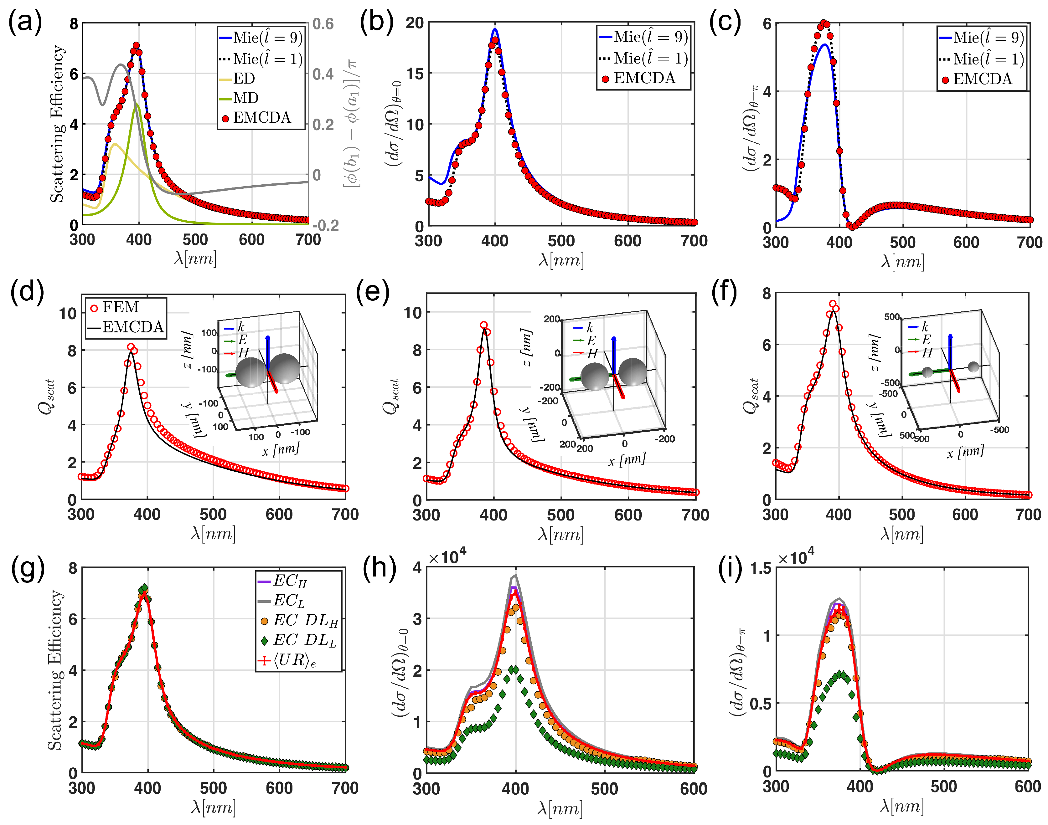
Before analyzing the scattering properties of the arrays, we performed different benchmarks of the EMCDA method with respect to the analytical full-wave Mie theory [88,89] applied to a single TiO${}_2$ nanoparticle with a radius of 70 nm. Figure 13a–c show the results of this comparison. In particular, Figure 13a displays the scattering efficiency computed using the analytical Mie–Lorentz theory by truncating the multipolar expansion up to the convergence order provided by $\widehat{l}=x+4.05x^{1/3}+2$ [87] (x is the size parameter) as compared to both the analytical result with only the dipolar contribution ($\widehat{l}=1$) and the numerical EMCDA calculation (red circle markers). The agreements between the EMCDA and the Mie theory with only the dipolar contribution is almost perfect. Moreover, the relative error due to the dipolar approximation, evaluated from the ratio of the area beyond the blue and the black dotted curves, is 1.5%. Therefore, the scattering properties of these small nanoparticles are sufficiently well-described by considering only the electric ($a_1$) and magnetic ($b_1$) dipole terms of the Mie expansion [79]. Figure 13b,c display, respectively, the differential scattering efficiency in the forward and backward direction evaluated by using Equations (35) and (36), respectively, (red circle markers) and compare to the results from the equations:

$$Q_{bs}^{Mie}=\frac{1}{{\left(k_{0}R\right)}^2}{\left|\sum _{l=1}^{\widehat{l}}(2l+1){(-1)}^l(a_l-b_l)\right|}^2{Q}_{fd}^{Mie}=\frac{1}{{\left(k_{0}R\right)}^2}{\left|\sum _{l=1}^{\widehat{l}}(2l+1)(a_l+b_l)\right|}^2$$

(38)

that are derived from the Mie theory [88,89] when $\widehat{l}=9$ (blue curve) and $\widehat{l}=1$ (dotted black line). Again, the matching between the EMCDA and the Mie theory with $\widehat{l}=1$ is excellent. On the other hand, the relative error due to the dipolar approximation is approximately 10% for both comparisons. This is due to the fact that the higher-order multipoles interfere with the dipole moments for fixed scattering directions. We remark that Equation (38) describes a coherent sum between all the multipole moments. On the other hand, no interference effects contribute to the total scattering efficiency [88]. Interestingly, Figure 13c shows that the backscattered light is completely suppressed around $\lambda \sim 420$ nm, where the relative phase between the electric ($\varphi \left(a_1\right)$) and magnetic ($\varphi \left(b_1\right)$) dipoles crosses zero, as shown in the grey y-axis of Figure 13a (see also [90] for more details).

In order to analyze the scattering properties of the $EC$ and $EC$$DL$ arrays, we have selected the structures that showed significantly different modal lifetime behavior. Namely, $E{C}_H$, $E{C}_L$, $EC$$D{L}_H$, and $EC$$D{L}_L$. To avoid the occurrence of overlapping nanoparticles (remember that we are considering now a real scattering object characterized by a size and a material through the polarizabilities expressed by Equation (19)), we have rescaled these aperiodic arrays by fixing the minimum particle separation to be of the order of $2R+10$ nm. We carefully verified the accuracy of the EMCDA simulations by comparing them with simulations performed using the finite element method (FEM) in a dimer nanoparticle configuration with 10 nm gap separation. The FEM model was meshed with 5.6 nm maximum element size and 0.56 nm minimum element size. The total degrees of freedom of the FEM simulation were 1,420,416. We performed the simulations using a 40 core cluster (Intel Xeon(R) CPU E5-2698 v4) with 256Gb total RAM. Typical time to complete full-spectrum simulations was approximately 4 h and only approximately 3 min using the EMCDA method on the same geometry. Moreover, the Green’s matrix spectral method provides fundamental physical information about the light transport properties of open scattering systems that cannot be easily accessed via other numerical methods, such as finite difference time domain (FDTD) or finite elements (FEM). Indeed, in contrast to numerical mesh-based methods, the Green’s matrix spectral method and its EMCDA extension allow one not only to obtain the frequency positions and lifetimes of all the scattering resonances, but also to fully characterize their spectral statistics and measurable scattering parameters. Finally, these methods enable the understanding of the full spectral characteristics of the deterministic aperiodic arrays containing several thousand interacting nanoparticles, which are well beyond the reach of mesh-based numerical methods.

The validation results (shown in Figure 13d–f for the longitudinal polarization) yield a small ($6\%$) discrepancy compared to the ones obtained using our EMCDA method. On the other hand, the results of the EMCDA analysis on the arrays are reported in Figure 13g–i. Since only a small fraction (<$5\%$) of the particles in the arrays are separated by the 10 nm minimum gap distance, the application of the EMCDA method to these geometries is fully justified and the contribution of higher-order electromagnetic multipoles can be safely neglected. Our findings show that the scattering spectra of the investigated $EC$ and $EC$$DL$ structures overlap very well with the spectrum of the ensemble-averaged $UR$ system across the entire visible spectrum. This is in agreement with the uncorrelated nature of the $EC$ arrays and of the $EC$$DL$ arrays with the largest and the smallest modal lifetimes. However, structural differences between these systems can be identified by considering the spectral behavior of their directional scattering parameters. This has been achieved by computing the forward and the backward scattering spectra, which are shown in Figure 13h,i, respectively. In particular, we observe that the data obtained on $EC$$D{L}_L$ feature significantly reduced forward and backscattering intensities, reflecting a more correlated spatial structure compared to all the other systems. Smaller differences are also visible among the other $EC$-based structures when compared to the ensemble-averaged $UR$ case.

In order to more precisely address the subtle modifications in the directional scattering parameters we analyzed in Figure 14 the linewidth and the maximal differential scattering efficiency in the backward direction for the different arrays. The analysis is performed considering 26 representative $EC$ and $EC$$DL$ structures. In order to uniformly sample the vast space of structural parameters that we have examined in the Section 3, we have selected 52 aperiodic arrays by using as discriminator the average modal lifetime $\widehat{\mathsf{\Gamma }}$, as reported in Figure 6 and Figure 11. Specifically, 26 $EC$ arrays were chosen between the 900 different elliptic curves point patterns generated by the integer coefficients A and B in the range (1, 30) ordered by following the trend of $\widehat{\mathsf{\Gamma }}$. Specifically, 26 different $EC$ structures were selected with parameter values that are equidistant between the $E{C}_L$ and the $E{C}_H$ structure. In the same way, the 26 $ECDL$ arrays were selected equidistantly between the 36 different structures discussed in Figure 11. All these 52 arrays were scaled to avoid the occurrence of overlapping nanoparticles.

Table 1. Averaged structural parameters of the different analyzed devices. Specifically, $d_{min}$, $d_1$ and $\rho$ indicates, respectively, the minimum particle separation, the averaged first-neighbor particle separation, and the particle density evaluated as $N/L_x{L}_y$ ($L_{x,y}$ are the lateral dimension along the x and y direction).

Structural Parameters	EC	EC DL	UR
$\langle d_{min}\rangle$$\left[nm\right]$	$152.04\pm 1.72$	$189.79\pm 19.35$	$151.05\pm 1.05$
$\langle d_1\rangle$$\left[nm\right]$	$482.99\pm 5.03$	$499.43\pm 12.69$	$484.11\pm 3.62$
$\rho$$\left[\mu m^{-2}\right]$	$1.22\pm 0.03$	$1.20\pm 0.11$	$1.23\pm 0.04$

summarizes the averaged structural parameters of all the investigated structures. All share approximately the same minimum and averaged first-neighbor particle separation, as well as the same particle density.

The normalized lineshapes of the backscattering are displayed in Figure 14a and show a significant variability. The backscattering of a $UR$ representative realization is also shown for comparison in red. The significant differences in the width of the backscattering angular spectrum (computed at the wavelength of maximum scattering) evidence subtle differences in the structural properties of the arrays that cannot otherwise be resolved by total scattering analysis. The more sensitive interference effects that contribute to the width and intensity of the backscattering cone allow us to differentiate between different $EC$ and $EC$$DL$ structures for the first time. Note that simply considering the maximum backscattering efficiency, shown in Figure 14b, would not lead to a clear discrimination between a $UR$ and the different $EC$ structures. The full-width-at-half-maximum (FWHM) results obtained for all the investigated structures are plotted in Figure 14c,d, which demonstrate a great variability across the analyzed sample. We should appreciate that the FWHM of the backscatering cone varies by almost a factor of two across the different $EC$$DL$ structures, which is evidence of significant modifications in the underlying geometrical structure of the arrays. Therefore, our findings not only establish that $EC$ and $EC$$DL$ are remarkably different from uniform random systems, but they may also provide an optical approach to rapidly identify the potential vulnerabilities of modern $EC$-based cryptosystems by investigating coherent light scattering effects in the associated photonic structures.

6. Conclusions

In this paper we introduce a novel class of deterministic aperiodic photonic systems that physically implement the distinctive aperiodic order of elliptic curves and their associated discrete logarithm problem. In particular, we addressed structure-property relationships in a large number (900) of aperiodic photonic systems that manifest an extremely rich spectrum of scattering and localization properties that can be engineered to outperform the performances of traditional uniform random media in terms of optical confinement and directional light scattering. By combining the interdisciplinary methods of point patterns spatial statistics with the rigorous Green’s matrix solution of the multiple wave scattering problem for electric and magnetic dipoles we systematically explored the spectral and light scattering properties of novel deterministic aperiodic structures with enhanced light-matter coupling for nanophotonics and metamaterials applications to imaging and spectroscopy. By demonstrating significant deviations from traditional random media, our findings not only underline the importance of structural correlations in elliptic curve-based structures for photonics technology but may additionally provide an optics-driven approach to rapidly identify potential vulnerabilities in modern EC-based cryptosystems.