Mechanical Analysis of Functionally Graded Multilayered Two-Dimensional Decagonal Piezoelectric Quasicrystal Laminates with Imperfect Interfaces

Abstract

Quasicrystals have a wide range of applications due to their unique multi-field coupling effects and distinctive physical and mechanical characteristics. In this paper, the static and dynamic problems of imperfectly bonded, multilayered, functionally graded, two-dimensional decagonal piezoelectric quasicrystal laminates under mixed boundary conditions are investigated. The state equations in a concise and compact matrix form can be expressed by using differential quadrature regional discrete point expansions in any layer of the laminate. This allows for the representation of displacement, stress, electric potential, and electric displacement components. Then, different imperfect interface conditions are introduced to characterize specific structural and electric contact properties at the bounding interfaces, which are further converted to the interface propagator matrix. Numerical examples are carried out to investigate the impact of varying interface compliances, load types, and functional gradient factors on the static bending and vibration phenomena of QC laminates. These results can be used as references to validate existing or future numerical work on QC laminates and could further guide the design of related QC laminate structures.

1. Introduction

Quasicrystals (QCs) were discovered by Shechtman [1] in 1982 during X-ray diffraction experiments on Al-Mn alloys. Natural QCs were first discovered in 2009 [2], followed by the discovery of natural QCs with decagonal symmetry in 2015 [3], proving that QCs are widespread in the natural environment. Until now, nearly 210 different natural and synthetic solid QC materials have been reported. QCs can be divided into one-(1D), two-(2D), and three-dimensional (3D) QCs according to the dimensionality of the atoms’ quasiperiodic arrangement [4]. Due to the special atomic arrangement and multi-field coupling effects, QCs possess various superb characteristics. The mathematical elasticity of solid and soft matter QCs and their related theories were systematically studied by Fan [5], who summarized various QC material parameters and methods for solving various problems. Piezoelectric quasicrystals (PQCs) refer to QCs with piezoelectric effects. PQCs can have various applications across different fields due to their unique combination of characteristics, such as sensors and actuators [6,7], electromechanical systems, acoustic devices, and so on. Since PQC materials have a wide range of applications, it is important to study the effect of piezoelectric and multi-field coupling on their mechanical properties [8,9,10,11], to enhance the exploration of their potential applications.

Due to the highly complex composition of QCs’ non-stoichiometric structure, the preparation of large-size QCs is very difficult. As such, QCs are often fabricated as layered structures with their mechanical behaviors being important in various engineering applications. Yang et al. [12] utilized the pseudo-Stroh formalism to provide an accurate solution for a multilayered 2D decagonal QC laminate with simply supported boundary conditions. Guo et al. [13] developed analytical solutions for the free and forced vibrations of a 1D QC nanoplate. Huang et al. [14] employed the state-space method (SSM) to study the behavior of compressible fluids that are filled with multilayered 2D PQC cylindrical shells. Huang et al. [15] examined the interlaminar stresses in piezoelectric composite laminates. Guo et al. [16] proposed a non-local analytical solution for FG multilayered 1D hexagonal PQC nanoplates.

Functional gradient materials (FGMs) consist of two or more materials with a gradual change in composition and structure. By gradually altering the volume fraction of the constituent materials, the mechanical properties in the FGMs can be tuned to smoothly and continuously vary from one surface to another. FGMs are widely used in laminates, especially in QC laminates, due to their designable characteristics. Vel et al. [17] obtained 3D accurate solutions of free and forced vibrations of FGM rectangular thick plates under simply supported boundary conditions. Phung-Van et al. [18] applied the generalized shear theory deformation principle to investigate the response of FGM piezoelectric plates under thermo-mechanical loading. Guo et al. [19] studied the scale effect in anisotropic and MEE FGM plates. Feng et al. [20] analyzed the effects of boundary conditions and functional gradient factors on the static solutions of 2D FGM QC plates.

In practice, however, internal defects and imperfect interfaces could exist in composites where the interfaces could be made of interfacial dislocations and/or cracks [21,22]. A common imperfect interface is the spring-type where the traction is linearly connected to the displacement jump [23]. Qu [24] modeled the imperfect interface with linear spring layers of unaccounted thickness and investigated the impact of imperfect interfaces on the overall elastic property of the composites using the Mori–Tanaka method. Shariyat [25] analyzed the non-linear bending and buckling of imperfect sandwich plates under thermo-mechanical loading using the generalized 3D higher-order double superposition theory. Chen et al. [26] used a general spring model to simulate imperfect interfaces and obtained an accurate 3D solution for a piezoelectric rectangular laminate with imperfect interfaces.

In 1971, Bellman [27] proposed the differential quadrature method (DQM) to solve boundary-value problems and found that the DQM could be very accurate by using only a few discrete points. DQM is a numerical technique used to solve both ordinary and partial differential equations. It is essentially a matching point method, which requires finding the corresponding discrete points in the solution region and replacing the derivatives of the original function at the discrete points with a linear combination of the function values at the discrete points and the corresponding weights. By applying DQM, Bert and Malik et al. [28] studied the free vibration of laminates under different boundary conditions and demonstrated that the computational space required in DQM is much less than that based on either the Fourier series method or the Rayleigh–Ritz method. Chen et al. [29] combined DQM with SSM, called SS-DQM, to deal with laminar structures with free boundaries, and studied a series of static bending and free vibration problems for laminated structures with complex boundary conditions and multi-field coupling. The SS-DQM was also used to solve the static bending and free vibration problems with different boundary conditions for piezoelectric, piezomagnetic, and other smart materials [30,31,32].

In this paper, a semi-analytical solution is derived for a layered PQC rectangular laminate with imperfect interfaces. It is based on the SS-DQM and propagator matrix method. This paper is organized as follows: Section 2 presents the governing equations for 2D decagonal PQCs based on the QC linear elasticity, introduces the DQM, and derives the solution to the state equations. Section 3 implements joint coupling matrices to avoid numerical instability at various discrete points. Section 4 derives the imperfect interface forms for elastic fields, as well as weakly (or highly) conducting dielectric interfaces. Section 5 studies the influence of interface compliances, functional gradient factors, and load types on the static and dynamic response of 2D PQC laminates.

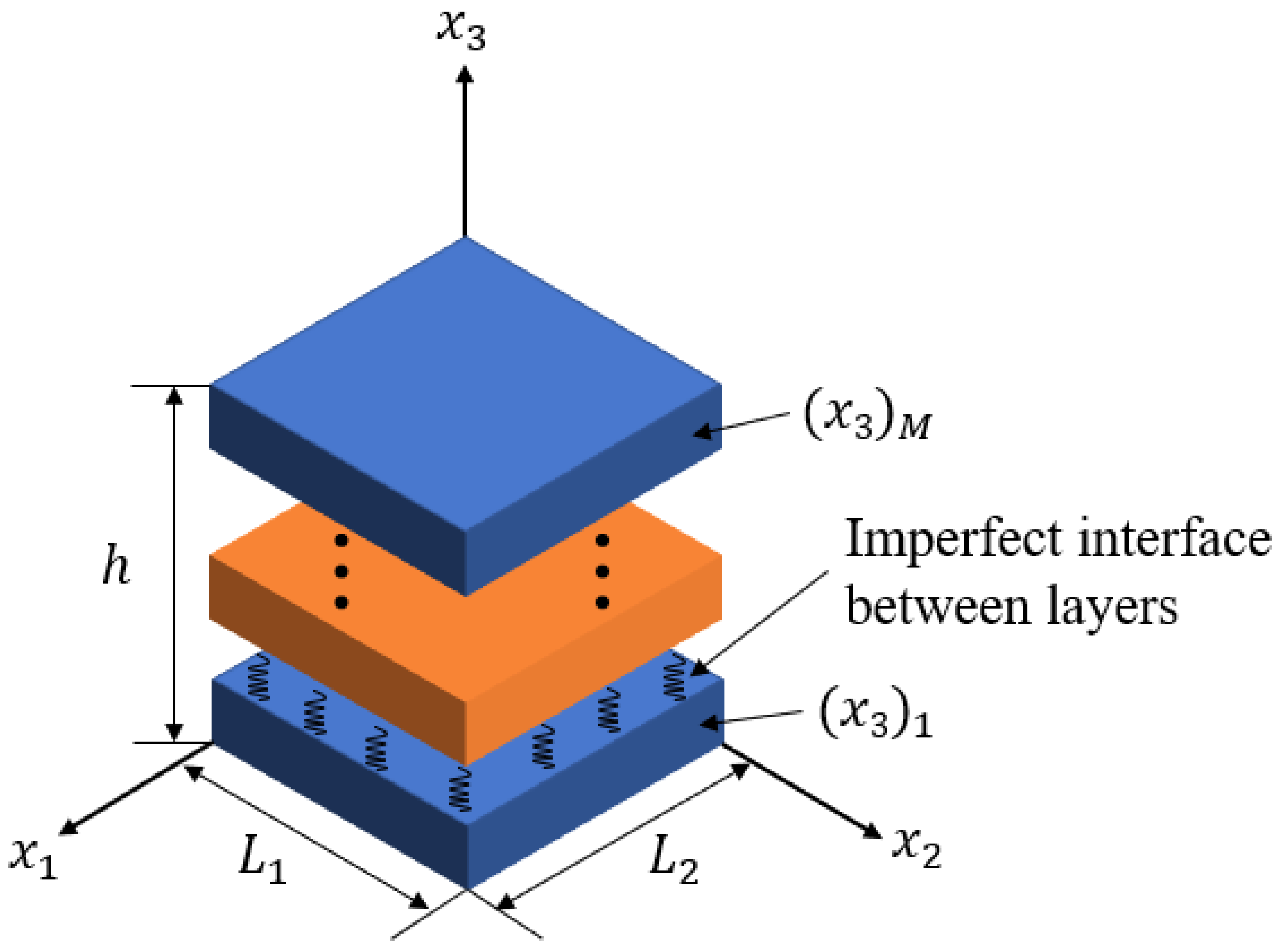
2. Description and Formulation of the Problem

Figure 1 is the problem geometry of a three-layered 2D PQC rectangular laminate with length L₁, width L₂, and height h in terms of a global and fixed Cartesian coordinate system (x, y, z) = (x₁, x₂, x₃). The thickness of each layer in the laminate, denoted as h_p (p = 1, 2, 3, …, M), is defined as the difference between the coordinates z_p and z_p−1. The generalized spring model is employed to represent the imperfect interface between adjacent layers. In this imperfect interface model, the tractions remain continuous across the interface, and they are further proportional to the displacement jumps via the interface “spring factor”. For the interface with weakly conducting dielectric, the electric displacement remains continuous, but the electric potential does not. The jump in the electric potential is proportional to the electric displacement. On the other hand, for the interface with highly conducting dielectric, the electric potential stays continuous, while there exists a discontinuity in the electric displacement, which is a function of the electric potential. The atomic arrangement of 2D PQC is quasiperiodic in the x₁-x₂ plane and periodic in the x₃-direction. The flat top and bottom surfaces are located at (x₃)_M = h and (x₃)₁ = 0, respectively.

2.1. Basic Equations

Based on the QC linear elasticity, the geometric equations of 2D PQCs are

$${\epsilon }_{ij}=\frac{1}{2}\left(\frac{\partial u_i}{\partial x_j}+\frac{\partial u_j}{\partial x_i}\right), w_{mj}=\frac{\partial w_m}{\partial x_j}, E_i=-\frac{\partial \varphi }{\partial x_i},$$

(1)

where ε_ij (i, j = 1, 2, 3) and w_mj (m = 1, 2) are the strains in the phonon and phason fields, respectively; u_i and w_m are the displacements in the phonon and phason fields, respectively; E_i stands for the electric field; and ϕ represents the electric potential.

The essence of FGMs is the continuous change of material properties in a certain direction. We assume that the material properties of FG QC materials are exponentially distributed along the x₃-direction. Therefore, the generalized constitutive equations [33] of 2D decagonal PQCs are

$$\begin{array}{l}{\sigma }_{11}=C_{11}\left(x_3\right){\epsilon }_{11}+C_{12}\left(x_3\right){\epsilon }_{22}+C_{13}\left(x_3\right){\epsilon }_{33}+R_1\left(x_3\right)\left(w_{11}+w_{22}\right)-e_{31}\left(x_3\right)E_3,\\ {\sigma }_{22}=C_{12}\left(x_3\right){\epsilon }_{11}+C_{11}\left(x_3\right){\epsilon }_{22}+C_{13}\left(x_3\right){\epsilon }_{33}-R_1\left(x_3\right)\left(w_{11}+w_{22}\right)-e_{31}\left(x_3\right)E_3,\\ {\sigma }_{33}=C_{13}\left(x_3\right){\epsilon }_{11}+C_{13}\left(x_3\right){\epsilon }_{22}+C_{33}\left(x_3\right){\epsilon }_{33}-e_{33}\left(x_3\right)E_3,\\ {\sigma }_{23}={\sigma }_{32}=2C_{44}\left(x_3\right){\epsilon }_{23}-e_{15}\left(x_3\right)E_2,\\ {\sigma }_{13}={\sigma }_{31}=2C_{44}\left(x_3\right){\epsilon }_{13}-e_{15}\left(x_3\right)E_1,\\ {\sigma }_{12}={\sigma }_{21}=2C_{66}\left(x_3\right){\epsilon }_{12}-R_1\left(x_3\right)w_{12}+R_1\left(x_3\right)w_{21},\\ H_{11}=R_1\left(x_3\right)\left({\epsilon }_{11}-{\epsilon }_{22}\right)+K_1\left(x_3\right)w_{11}+K_2\left(x_3\right)w_{22},\\ H_{22}=R_1\left(x_3\right)\left({\epsilon }_{11}-{\epsilon }_{22}\right)+K_1\left(x_3\right)w_{22}+K_2\left(x_3\right)w_{11},\\ H_{23}=K_4\left(x_3\right)w_{23},\\ H_{12}=-2R_1\left(x_3\right){\epsilon }_{12}+K_1\left(x_3\right)w_{12}-K_2\left(x_3\right)w_{21},\\ H_{13}=K_4\left(x_3\right)w_{13},\\ H_{21}=2R_1\left(x_3\right){\epsilon }_{12}+K_1\left(x_3\right)w_{21}-K_2\left(x_3\right)w_{12},\\ D_1=2e_{15}\left(x_3\right){\epsilon }_{13}+{\xi }_{11}\left(x_3\right)E_1,\\ D_2=2e_{15}\left(x_3\right){\epsilon }_{23}+{\xi }_{22}\left(x_3\right)E_2,\\ D_3=e_{31}\left(x_3\right)\left({\epsilon }_{11}+{\epsilon }_{22}\right)+e_{33}\left(x_3\right){\epsilon }_{33}+{\xi }_{33}\left(x_3\right)E_3,\end{array}$$

(2)

where σ_ij and H_mj are the stresses in the phonon and phason fields, respectively; D_i stand for the electric displacements; C_ij, C_44, and C₆₆ = (C₁₁ − C₁₂)/2 (in N/m²) are the elastic constants in the phonon field; K₁, K₂, and K₄ (in N/m²) represent the phason elastic constants; R₁ (in N/m²) represents the phonon–phason coupling elastic constant; ξ_ii (in C²/(N∙m²)) represent the dielectric coefficients; and e₁₅, e₃₁, and e₃₃ (in C/m²) represent the piezoelectric coefficients in the phonon field. Each material parameter is a function of x₃, assuming that the material parameters vary exponentially along the x₃ axis, i.e.,

$$\begin{array}{l}{C}_{ij}\left(x_3\right)=C_{ij}^0{\mathrm{e}}^{\eta x_3},R_1\left(x_3\right)=R_1^0{\mathrm{e}}^{\eta x_3},K_m\left(x_3\right)=K_m^0{\mathrm{e}}^{\eta x_3},{\xi }_{ii}\left(x_3\right)={\xi }_{ii}{\mathrm{e}}^{\eta x_3},\\ e_{11}\left(x_3\right)=e_{11}^0{\mathrm{e}}^{\eta x_3},e_{15}\left(x_3\right)=e_{15}^0{\mathrm{e}}^{\eta x_3},e_{33}\left(x_3\right)=e_{33}^0{\mathrm{e}}^{\eta x_3},\end{array}$$

(3)

where the superscript “0” represents the material parameters at the bottom of each layer, and η is the gradient factor.

The equilibrium equations of 2D PQCs, in the absence of body force and electric charge densities, can be expressed based on Newton’s second law and Bak’s theory [34,35]

$${\sigma }_{ij,j}=0, H_{mj,j}=0, D_{j,j}=0.$$

(4)

Regarding the dynamic behavior of QCs, there are various arguments due to the unclear physical phenomenon on the phason field, as compared to the statics. Lubensky et al. [36] proposed that the phason field, unlike the phonon field, does not respond to spatial translations and exhibits diffusive behavior with significantly longer diffusion times. Building upon this concept, they introduced the hydrodynamics model for QCs. However, Bak [34] pointed out a different perspective, suggesting that both the phonon and phason fields behave similarly in dynamics, following the acoustic modes. Ding et al. [37], based on Bak’s theory, examined the equation of motion for QCs and found that the law of momentum conservation applies to both phonons and phasons. In this paper, we use the elastodynamics model with wave type to investigate the dynamic behavior of QCs. Therefore, the motion equations of 2D PQCs in the absence of body force and electric charge densities following the elastodynamics model of wave type [37,38] can be expressed as

$${\sigma }_{ij,j}=\rho u_{i,tt}, H_{mj,j}=\rho w_{m,tt}, D_{j,j}=0,$$

(5)

where $\rho$ is the desity of the 2D PQCs.

2.2. State Equations of a Homogeneous QC Laminate Layer

Substituting Equation (1) into Equation (2) and combining with Equation (4) or Equation (5), the partial differential state equations are

$$\frac{\partial }{\partial x_3}{\xi }_1=D{\xi }_1,$$

(6)

where state variable ξ₁ = [u₁, u₂, u₃, w₁, w₂, ϕ, σ₃₃, σ₂₃, σ₁₃, H₂₃, H₁₃, D₃]^T, and D is the state matrix, which has different forms in the static and dynamic cases. The specific forms of the equations for both the static and dynamic cases are given in the Appendix A.1 and Appendix A.2.

For the electro-elastic problem of a 2D PQC laminate, the simply supported and electrically grounded boundary conditions are

$$u_{2,i}=u_{3,i}=0, {\sigma }_{11,i}=H_{11,i}=0, \varphi =0.$$

(7)

To satisfy the simply supported boundary conditions (Equation (7)), we assume the following general solutions in the form of Fourier series expansions for displacements, stresses, electric potential, and electric displacements (for the time-harmonic case)

$$\left[\begin{array}{l}{u}_1\\ u_2\\ u_3\\ w_1\\ w_2\\ \varphi \end{array}\right]={\displaystyle \sum _{m=1}^{\infty }{\displaystyle \sum _{n=1}^{\infty }\left[\begin{array}{l}{u}_{1mn}\cos (p{x}_1)\sin (q{x}_2)\\ u_{2mn}\sin (p{x}_1)\cos (q{x}_2)\\ u_{3mn}\sin (p{x}_1)\sin (q{x}_2)\\ w_{1mn}\cos (p{x}_1)\sin (q{x}_2)\\ w_{2mn}\sin (p{x}_1)\cos (q{x}_2)\\ {\varphi }_{mn} \sin (p{x}_1)\sin (q{x}_2)\end{array}\right]}}{e}^{i\omega t},\left[\begin{array}{l}{\sigma }_{33}\\ {\sigma }_{23}\\ {\sigma }_{13}\\ H_{23}\\ H_{13}\\ D_3\end{array}\right]={\displaystyle \sum _{m=1}^{\infty }{\displaystyle \sum _{n=1}^{\infty }\left[\begin{array}{l}{\sigma }_{33mn}\sin (p{x}_1)\sin (q{x}_2)\\ {\sigma }_{23mn}\sin (p{x}_1)\cos (q{x}_2)\\ {\sigma }_{13mn}\cos (p{x}_1)\sin (q{x}_2)\\ H_{23mn}\sin (p{x}_1)\cos (q{x}_2)\\ H_{13mn}\cos (p{x}_1)\sin (q{x}_2)\\ D_{3mn}\sin (p{x}_1)\sin (q{x}_2)\end{array}\right]}}{e}^{i\omega t},$$

(8)

where the imaginary $\mathrm{i}=\sqrt{-1}$; p = mπ/L₁, q = nπ/L₂, in which m, n is the half-wave number taking only positive integers; and ω is the angular frequency. And ω is the angular frequency. The above general solutions apply to the dynamic case, while the static case can be obtained by letting ω = 0.

By substituting Equation (8) into Equation (6), Equation (6) is transformed from partial differential equations (PDEs) to ordinary differential equations (ODEs). However, the double Fourier series expansion form can only satisfy the simply supported boundary condition, but no longer be applicable if there are clamped or mixed boundary conditions.

Assume that the laminate is simply supported at x₂ = 0 and x₂ = L₂, and the other two edges are random boundary conditions, then, each quantity can only be expanded in the Fourier series along the x₂-direction

$$\left[\begin{array}{l}{u}_1\\ u_2\\ u_3\\ w_1\\ w_2\\ \varphi \end{array}\right]={\displaystyle \sum _{n=1}^{\infty }\left[\begin{array}{l}{u}_{1n}\sin (q{x}_2)\\ u_{2n}\cos (q{x}_2)\\ u_{3n}\sin (q{x}_2)\\ w_{1n}\sin (q{x}_2)\\ w_{2n}\cos (q{x}_2)\\ {\varphi }_n \sin (q{x}_2)\end{array}\right]}{e}^{i\omega t},\left[\begin{array}{l}{\sigma }_{33}\\ {\sigma }_{23}\\ {\sigma }_{13}\\ H_{23}\\ H_{13}\\ D_3\end{array}\right]={\displaystyle \sum _{n=1}^{\infty }\left[\begin{array}{l}{\sigma }_{33n}\sin (q{x}_2)\\ {\sigma }_{23n}\cos (q{x}_2)\\ {\sigma }_{13n}\sin (q{x}_2)\\ H_{23n}\cos (q{x}_2)\\ H_{13n}\sin (q{x}_2)\\ D_{3n}\sin (q{x}_2)\end{array}\right]}{e}^{i\omega t}.$$

(9)

Substituting Equation (9) into Equation (6), we obtain Equation (A1) (the exact form is given in Appendix A.4). It should be noted that Equation (A1) is still partial differential equations (PDEs) and cannot be solved analytically. Therefore, the DQM is used to solve the PDEs. DQM can approximate the derivative of a function with respect to a direction by a linear combination of the weight coefficients and the values of the original function at the discrete points. Therefore, the n-order derivative of a function f (x₁, x₃) at a discrete point in the Cartesian coordinate system at x = x_{1, i} is

$${\left.\frac{{\partial }^{n}f\left(x_1,x_3\right)}{\partial x_1^n}\right|}_{x_1=x_{1,i}}={\displaystyle \sum _{k=1}^N{X}_{ik}^{(n)}f\left(x_{1,k},x_3\right)},$$

(10)

where $X_{ik}^{\left(n\right)}$ are the differential quadrature weight coefficients; and N is the number of discrete points in the x₁-direction. The weighting coefficients along the x₁-direction are calculated using the polynomial expansion form as

$$\left\{\begin{array}{l}{X}_{ik}^{(1)}=\frac{{\displaystyle {\prod }_{r=1,r\ne i}^N\left(x_i-x_r\right)}}{\left(x_i-x_k\right){\displaystyle {\prod }_{r=1,r\ne k}^N\left(x_k-x_r\right)}}\left(i\ne k\right),\\ X_{ii}^{(1)}=-{\displaystyle \sum _{k=1,k\ne i}^N{X}_{ik}^{(1)}},\\ X_{ik}^{(2)}={\displaystyle \sum _{r=1}^N{X}_{ir}^{(1)}{X}_{rk}^{(1)}}.\end{array}\right.$$

(11)

Also, the form of Chebyshev–Gauss–Lobatto discrete points is used to represent the distribution of discrete points in the discrete domain

$$x_{1,i}=\frac{L_1}{2}\left[1-\cos \left(\frac{i-1}{N-1}\pi \right)\right]i=1,2,\dots N.$$

(12)

By expanding the stresses, displacements, electric potential, and electric displacements in Equation (6) using the Fourier series and DQM, for static problem, we obtain the following set of state equations

$$\begin{array}{l}\frac{d{u}_{1,i}}{d{x}_3}=-{\displaystyle \sum _{k=1}^N{X}_{ik}^{\left(1\right)}}{u}_{3,k}-a_1{\displaystyle \sum _{k=1}^N{X}_{ik}^{\left(1\right)}}{\varphi }_{,k}+a_2{\sigma }_{13,i},\\ \frac{d{u}_{2,i}}{d{x}_3}=-q{u}_{3,i}-a_{1}q{\varphi }_{,i}+a_2{\sigma }_{23,i},\\ \frac{d{u}_{3,i}}{d{x}_3}=-{\displaystyle \sum _{k=1}^N{X}_{ik}^{\left(1\right)}}{u}_{1,k}+\frac{a_4}{a_3}q{u}_{2,i}+\frac{a_5}{a_3}\sigma {}_{33,i}+\frac{a_6}{a_3}{D}_{3,i},\\ \frac{d{w}_{1,i}}{d{x}_3}=a_7{H}_{13,i},\\ \frac{d{w}_{2,i}}{d{x}_3}=a_7{H}_{23,i}, \\ \frac{d{\varphi }_{,i}}{d{x}_3}=\frac{a_8}{a_3}{\displaystyle \sum _{k=1}^N{X}_{ik}^{\left(1\right)}}{u}_{1,k}-\frac{a_8}{a_3}q{u}_{2,i}+\frac{a_6}{a_3}\sigma {}_{33,i}-\frac{a_9}{a_3}{D}_{3,i}, \\ \frac{d{\sigma }_{33,i}}{d{x}_3}=q{\sigma }_{23,i}-{\displaystyle \sum _{k=1}^N{X}_{ik}^{\left(1\right)}}{\sigma }_{13,k},\\ \frac{d{\sigma }_{23,i}}{d{x}_3}=\left(\frac{a_{10}}{a_3}-a_{12}-a_{13}\right)q{\displaystyle \sum _{k=1}^N{X}_{ik}^{\left(1\right)}}{u}_{1,k}-a_{13}{\displaystyle \sum _{k=1}^N{X}_{ik}^{\left(2\right)}}{u}_{2,k}-\left(\frac{a_{10}}{a_3}-a_{11}\right)q^2{u}_{2,i}^2\\ \hspace{1em}\hspace{1em}\hspace{1em}+2a_{14}q{\displaystyle \sum _{k=1}^N{X}_{ik}^{\left(1\right)}}{w}_{1,k}-a_{14}{\displaystyle \sum _{k=1}^N{X}_{ik}^{\left(2\right)}}{w}_{2,k}-a_{14}{q}^2{w}_{2,i}^2-\frac{a_4}{a_3}q{\sigma }_{33,i}+\frac{a_8}{a_3}q{D}_{3,i},\\ \frac{d{\sigma }_{13,i}}{d{x}_3}=a_{13}{q}^2{u}_{1,i}^2+\left(\frac{a_{10}}{a_3}-a_{11}\right){\displaystyle \sum _{k=1}^N{X}_{ik}^{\left(2\right)}}{u}_{1,k}+\left(\frac{a_{10}}{a_3}-a_{12}-a_{13}\right)q{\displaystyle \sum _{k=1}^N{X}_{ik}^{\left(1\right)}}{u}_{2,k}\\ \hspace{1em}\hspace{1em}\hspace{1em}-a_{14}{\displaystyle \sum _{k=1}^N{X}_{ik}^{\left(2\right)}}{w}_{1,k}-a_{14}{q}^2{w}_{1,i}^2+2a_{14}q{\displaystyle \sum _{k=1}^N{X}_{ik}^{\left(1\right)}}{w}_{2,k}\\ \hspace{1em}\hspace{1em}\hspace{1em}-\frac{a_4}{a_3}{\displaystyle \sum _{k=1}^N{X}_{ik}^{\left(1\right)}}{\sigma }_{33,k}+\frac{a_8}{a_3}{\displaystyle \sum _{k=1}^N{X}_{ik}^{\left(1\right)}}{D}_{3,k},\\ \frac{d{H}_{23,i}}{d{x}_3}=-2a_{14}q{\displaystyle \sum _{k=1}^N{X}_{ik}^{\left(1\right)}}{u}_{1,k}-a_{14}{\displaystyle \sum _{k=1}^N{X}_{ik}^{\left(2\right)}}{u}_{2,k}-a_{14}{q}^2{u}_{2,i}^2-a_{15}{\displaystyle \sum _{k=1}^N{X}_{ik}^{\left(2\right)}}{w}_{2,k}+a_{15}{q}^2{w}_{2,i}^2, \\ \frac{d{H}_{13}}{d{x}_3}=-a_{14}{\displaystyle \sum _{k=1}^N{X}_{ik}^{\left(2\right)}}{u}_{1,k}-a_{14}{q}^2{u}_{1,i}^2-2a_{14}q{\displaystyle \sum _{k=1}^N{X}_{ik}^{\left(1\right)}}{u}_{2,k}-a_{15}{\displaystyle \sum _{k=1}^N{X}_{ik}^{\left(2\right)}}{w}_{1,k}+a_{15}{w}_{1,i}^2, \\ \frac{d{D}_3}{d{x}_3}=\left(a_{16}+a_{17}\right){\displaystyle \sum _{k=1}^N{X}_{ik}^{\left(2\right)}}{\varphi }_{,k}-\left(a_{16}+a_{17}\right)q^2{\varphi }_{,i}^k+a_{1}q{\sigma }_{23,i}-a_1{\displaystyle \sum _{k=1}^N{X}_{ik}^{\left(1\right)}}{\sigma }_{13,k},\end{array}$$

(13)

where i = 1, 2, …, N, and the involved coefficients a_m are listed in Appendix A.3. By using the same way, applying Equations (10)–(12) into Equation(A2), we can get the state equations for dynamic problem.

Equation (13) represents the state equations at the endpoints when i = 1 and N. Therefore, we can express the simply supported (Equation (14)) and clamped (Equation (15)) boundary conditions directly in terms of displacements, stresses, and electric potential

$$u_{2,d}=u_{3,d}=0, {\sigma }_{11,d}=H_{11,d}=0, {\varphi }_{,d}=0,$$

(14)

$$u_{1,d}=u_{2,d}=u_{3,d}=w_{1,d}=w_{2,d}=0, {\varphi }_{,d}=0,$$

(15)

where d = 1 and N. Substituting the boundary conditions into Equation (13), the governing equations with relevant boundary conditions can be solved, as presented below.

To simplify the presentation, we introduce the following abbreviations for the boundary conditions of the laminate. Taking the 2D PQC laminates with SSSS and CCCC boundary conditions as examples, ‘SSSS’ denotes that the boundary condition is simply supported along the edges x₁ = 0, x₁ = L₂, x₂ = 0, and x₂ = L₁, and ‘CCCC’ indicates that the boundary condition is clamped along the edges x₁ = 0, x₁ = L₂, x₂ = 0, and x₂ = L₁. The state equations of these two boundary conditions are shown in Equations (A5) and (A6), respectively.

As such, Equation (13) for any layer, saying Layer p, can be simplified to a matrix form as

$$\frac{\mathrm{d}}{\mathrm{d}{x}_3}{\zeta }^{\left(p\right)}=P^{\left(p\right)}{\zeta }^{\left(p\right)},$$

(16)

where ${\zeta }^{\left(p\right)}={\left[u_1^T,u_2^T,u_3^T,w_1^T,w_2^T,{\varphi }^T,{\sigma }_{33}^T,{\sigma }_{23}^T,{\sigma }_{13}^T,H_{23}^T,H_{13}^T,D_3^T\right]}^T$, ${\mathrm{u}}_1^{\mathrm{T}}={ \stackrel{\mathrm{~}}{\mathrm{u}}}_{1\mathrm{i}}$; P^(p) is the coefficient matrix of Layer p.

3. General Solutions for a 2D QC Laminate

The state equations can be described as a system of homogeneous linear ODEs with constant coefficients. Due to their linear nature, it is possible to obtain the general solutions of these equations directly.

Based on the solution theory of ODEs, the general solutions of Equation (16) are

$${\zeta }^{\left(p\right)}\left(z\right)=\exp \left[\left(z-z_{p-1}\right)P^{\left(p\right)}\right]{\zeta }^{\left(p\right)}\left(z_{p-1}\right) \left(z_{p-1}\le z\le z_p\right),$$

(17)

where z_p−1 and z_p, respectively, represent the coordinates of the lower and upper interfaces of Layer p. Let z = z_p, we have

$${\zeta }_1^{\left(p\right)}=G^{\left(p\right)}{\zeta }_0^{\left(p\right)},$$

(18)

where ${\mathrm{G}}^{\left(p\right)}=\exp [{\stackrel{\_}{h}}_p{P}^{\left(p\right)}]$, in which ${\stackrel{\_}{h}}_p=z_p-z_{p-1}$, ${\xi }_1^{\left(p\right)}={\xi }^{\left(p\right)}(z_p)$, ${\xi }_0^{\left(p\right)}={\xi }^{\left(p\right)}(z_{p-1})$, subscripts 0 and 1 represent the lower and upper interfaces of Layer p. Similarly, let z = z_p+1, we have

$${\zeta }_1^{\left(p+1\right)}=G^{\left(p+1\right)}{\zeta }_0^{\left(p+1\right)}.$$

(19)

In the case of perfectly connected layers, all variables are continuous at their common interface

$${\zeta }_0^{\left(p+1\right)}={\zeta }^{\left(p+1\right)}\left(z_p\right)={\zeta }^{\left(p\right)}\left(z_p\right)={\zeta }_1^{\left(p\right)}.$$

(20)

Substituting Equation (20) into Equations (18) and (19) and eliminating the state variables on their common interface z_p, we obtain

$${\zeta }_1^{\left(p+1\right)}=G^{\left(p+1\right)}{G}^{\left(p\right)}{\zeta }_0^{\left(p\right)}.$$

(21)

For the entire multilayered laminate, when all the interfaces are perfectly connected, we have

$${\zeta }_1^{\left(k\right)}=G{\zeta }_0^{\left(1\right)},$$

(22)

where

$$G=G^{\left(k\right)}\cdots G^{\left(p+1\right)}{G}^{\left(p\right)}\cdots G^{\left(1\right)}={\displaystyle {\prod }_{p=k}^1{G}^{\left(p\right)}},$$

(23)

and Equation (23) is called the global propagator matrix.

Separating the displacements and stresses of the above equation, we obtain

$${\left\{\begin{array}{c}U\\ T\end{array}\right\}}_1^{\left(k\right)}=\left[\begin{array}{cc}{G}_{11}& G_{12}\\ G_{21}& G_{22}\end{array}\right]{\left\{\begin{array}{c}U\\ T\end{array}\right\}}_0^{\left(1\right)},$$

(24)

where $U=\left[u_1^T,u_2^T,u_3^T,w_1^T,w_2^T,{\varphi }^T\right]$, $T=\left[{\sigma }_{33}^T,{\sigma }_{23}^T,{\sigma }_{13}^T,H_{23}^T,H_{13}^T,D_3^T\right]$.

Then, from Equation (24), we have

$$U_1^{\left(k\right)}=G_{11}{U}_0^{\left(1\right)}+G_{12}{T}_0^{\left(1\right)},$$

(25)

$$G_{21}{U}_0^{\left(1\right)}=T_1^{\left(k\right)}-G_{22}{T}_0^{\left(1\right)}.$$

(26)

The above procedure is the same when solving static and dynamic problems. For the case of free vibration, assume the tractions and electric displacements on the top and bottom surfaces of the layered plate are zero. The frequency equation is obtained as

$$\left|G_{21}\right|=0.$$

(27)

Then, the natural frequencies of different orders can be obtained by solving its eigenvalues.

For the static problem, we assume that the mechanical loads acting on the top and bottom surfaces of the laminate can be expressed as

$$T_1^{\left(k\right)}={\overline{q}}_t, T_0^{\left(1\right)}={\overline{q}}_b,$$

(28)

where ${\stackrel{\_}{\mathrm{q}}}_{\mathrm{t}}$ and ${\stackrel{\_}{\mathrm{q}}}_{\mathrm{b}}$ represent the mechanical loads on the top and bottom surfaces, respectively.

Substituting Equation (28) into Equations (25) and (26), we obtain

$$U_1^{\left(k\right)}=G_{11}{U}_0^{\left(1\right)}+G_{12}{\overline{q}}_b,$$

(29)

$$G_{21}{U}_0^{\left(1\right)}={\overline{q}}_t-G_{22}{\overline{q}}_b.$$

(30)

The displacements and electric potential on the bottom surface can be obtained from Equation (30)

$$U_0^{\left(1\right)}=G_{21}^{-1}\left({\overline{q}}_t-G_{22}{\overline{q}}_b\right),$$

(31)

With these solutions, the state vectors at any thickness position in the laminate can be obtained using Equation (22).

4. Imperfect Conductive Interface Analysis

The interface of PQC laminates can be in an intermediate state between firmly bonded and completely debonded at the interfacial joints due to defects such as damage or cracks. On both sides of such an interface, the displacements or stresses are always discontinuous, and such an interface is called an imperfect interface. It is assumed that the traction at the interface is continuous, but the displacement is discontinuous. The imperfect condition on the interface for the elastic field can be expressed as follows

$$\begin{array}{l}{\left({\sigma }_{13}\right)}^{\left(p+1\right)-}={\left({\sigma }_{13}\right)}^{\left(p\right)+}=\left({\left(u_1\right)}^{\left(p+1\right)-}-{\left(u_1\right)}^{\left(p\right)+}\right){\alpha }_1^{\left(p\right)},\\ {\left({\sigma }_{23}\right)}^{\left(p+1\right)-}={\left({\sigma }_{23}\right)}^{\left(p\right)+}=\left({\left(u_2\right)}^{\left(p+1\right)-}-{\left(u_2\right)}^{\left(p\right)+}\right){\alpha }_2^{\left(p\right)},\\ {\left({\sigma }_{33}\right)}^{\left(p+1\right)-}={\left({\sigma }_{33}\right)}^{\left(p\right)+}=\left({\left(u_3\right)}^{\left(p+1\right)-}-{\left(u_3\right)}^{\left(p\right)+}\right){\alpha }_3^{\left(p\right)},\\ {\left(H_{13}\right)}^{\left(p+1\right)-}={\left(H_{13}\right)}^{\left(p+\right)}=\left({\left(w_1\right)}^{\left(p+1\right)-}-{\left(w_1\right)}^{\left(p\right)+}\right){\beta }_1^{\left(p\right)},\\ {\left(H_{23}\right)}^{\left(p+1\right)-}={\left(H_{23}\right)}^{\left(p\right)+}=\left({\left(w_2\right)}^{\left(p+1\right)-}-{\left(w_2\right)}^{\left(p\right)+}\right){\beta }_2^{\left(p\right)},\end{array}$$

(32)

where “−” and “+” are the quantities on the two sides of the common interface z_p between Layer p + 1 and Layer p; and ${\mathsf{\alpha }}_i^{\left(p\right)}$ and ${\mathsf{\beta }}_m^{\left(p\right)}$ are the interface-stiffness coefficients of the phonon and phason fields on the interface. It is noted that ${\mathsf{\alpha }}_i^{\left(p\right)},{\mathsf{\beta }}_m^{\left(p\right)}\to 0$ represents a completely separated interface, while ${\mathsf{\alpha }}_i^{\left(p\right)}, {\mathsf{\beta }}_m^{\left(p\right)}\to \infty$ denotes a perfectly connected interface.

The imperfect condition of the electric field can be categorized into two cases: dielectrically weakly and highly conducting. In the weakly conducting case (Equation (33)), it is assumed that the electric displacements on the interface are continuous while the electric potential is not.

$${\left(D_3\right)}^{\left(p+1\right)-}={\left(D_3\right)}^{\left(p\right)+}=\left({\left(\varphi \right)}^{\left(p+1\right)-}-{\left(\varphi \right)}^{\left(p\right)+}\right)\left(-{\gamma }_2^{(p)}\right).$$

(33)

In the highly conducting case (Equation (34)), the electric potential is continuous while the electric displacements are not.

$${\left(\varphi \right)}^{\left(p+1\right)-}={\left(\varphi \right)}^{\left(p\right)+}=\left({\left(D_3\right)}^{\left(p+1\right)-}-{\left(D_3\right)}^{\left(p\right)+}\right)\frac{1}{\Delta }{\gamma }_1^{\left(p\right)},$$

(34)

where Δ = ∂²/$x_1^2$ + ∂²/$x_2^2$, ${\mathsf{\gamma }}_m^{\left(p\right)}$ are the stiffness coefficients of the electric field. Now by ordering Equations (32)–(34) according to their orders in terms of ${\mathsf{\xi }}_1$, we have

$${\zeta }_1^{\left(p+1\right)-}=J^{\left(p\right)}{\zeta }_1^{\left(p\right)+},$$

(35)

where I is the identity matrix

$$J^{\left(p\right)}=\left[\begin{array}{cc}I& J_{12}^{\left(p\right)}\\ J_{21}^{\left(p\right)}& I\end{array}\right].$$

(36)

In the case of a dielectrically weakly conducting interface, we have

$$J_{21}^{\left(p\right)}=0_{6\times 6},$$

(37)

$$J_{12}^{\left(p\right)}=\mathrm{diag}\left[1/{\alpha }_1^{\left(p\right)}{I}_1\hspace{1em}1/{\alpha }_2^{\left(p\right)}{I}_2\hspace{1em}1/{\alpha }_3^{\left(p\right)}{I}_3\hspace{1em}1/{\beta }_1^{\left(p\right)}{I}_4\hspace{1em}1/{\beta }_2^{\left(p\right)}{I}_5\hspace{1em}-1/{\gamma }_2^{\left(p\right)}{I}_6\right].$$

(38)

In the case of dielectrically highly conducting, we have

$$J_{21}^{\left(p\right)}=\mathrm{diag}\left[0\hspace{1em}0\hspace{1em}0\hspace{1em}0\hspace{1em}0\hspace{1em}1/{\gamma }_1^{\left(p\right)}\Delta I_6\right],$$

(39)

$$J_{12}^{\left(p\right)}=\mathrm{diag}\left[1/{\alpha }_1^{\left(p\right)}{I}_1\hspace{1em}1/{\alpha }_2^{\left(p\right)}{I}_2\hspace{1em}1/{\alpha }_3^{\left(p\right)}{I}_3\hspace{1em}1/{\beta }_1^{\left(p\right)}{I}_4\hspace{1em}1/{\beta }_2^{\left(p\right)}{I}_5\hspace{1em}0\right].$$

(40)

If the laminate is perfectly connected, ${\mathbf{J}}_{12}^{\left(p\right)}={\mathbf{J}}_{21}^{\left(p\right)}=\mathbf{0}$.

In the following numerical studies, we further assume that

$$\frac{1}{{\alpha }_1^{\left(p\right)}}=\frac{1}{{\alpha }_2^{\left(p\right)}}=\frac{1}{{\alpha }_3^{\left(p\right)}}=\frac{1}{{\beta }_1^{\left(p\right)}}=\frac{1}{{\beta }_2^{\left(p\right)}}=\frac{1}{{\gamma }_1^{\left(p\right)}}=\frac{1}{{\gamma }_2^{\left(p\right)}}=\delta ,$$

(41)

where the interface compliance δ is used to characterize the degree of interface imperfection.

For the imperfect interface case, Equation (22) can be rewritten as follows

$${\zeta }_1^{\left(k\right)}={\displaystyle {\prod }_{p=k}^1{J}^{\left(p\right)}\left(h_p\right)}{G}^{\left(p\right)}{\zeta }_0^{\left(1\right)}.$$

(42)

In summary, the partial differential state equations are obtained through the state-space method. By using DQM and Fourier series expansions, they are modified to an ordinary differential form. Then, the imperfect interfaces are considered and the general solutions are obtained.

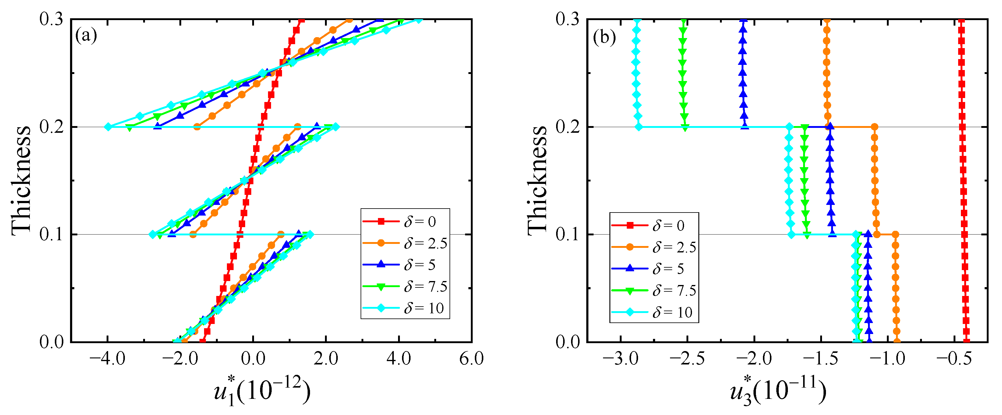
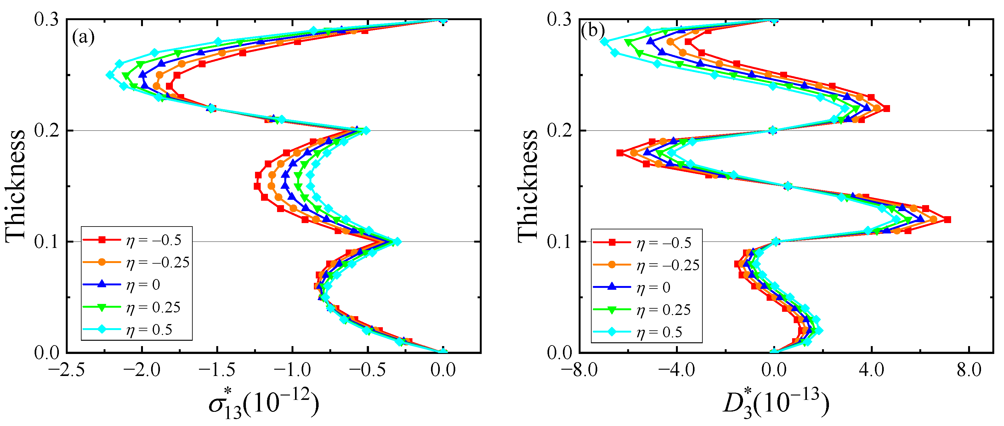
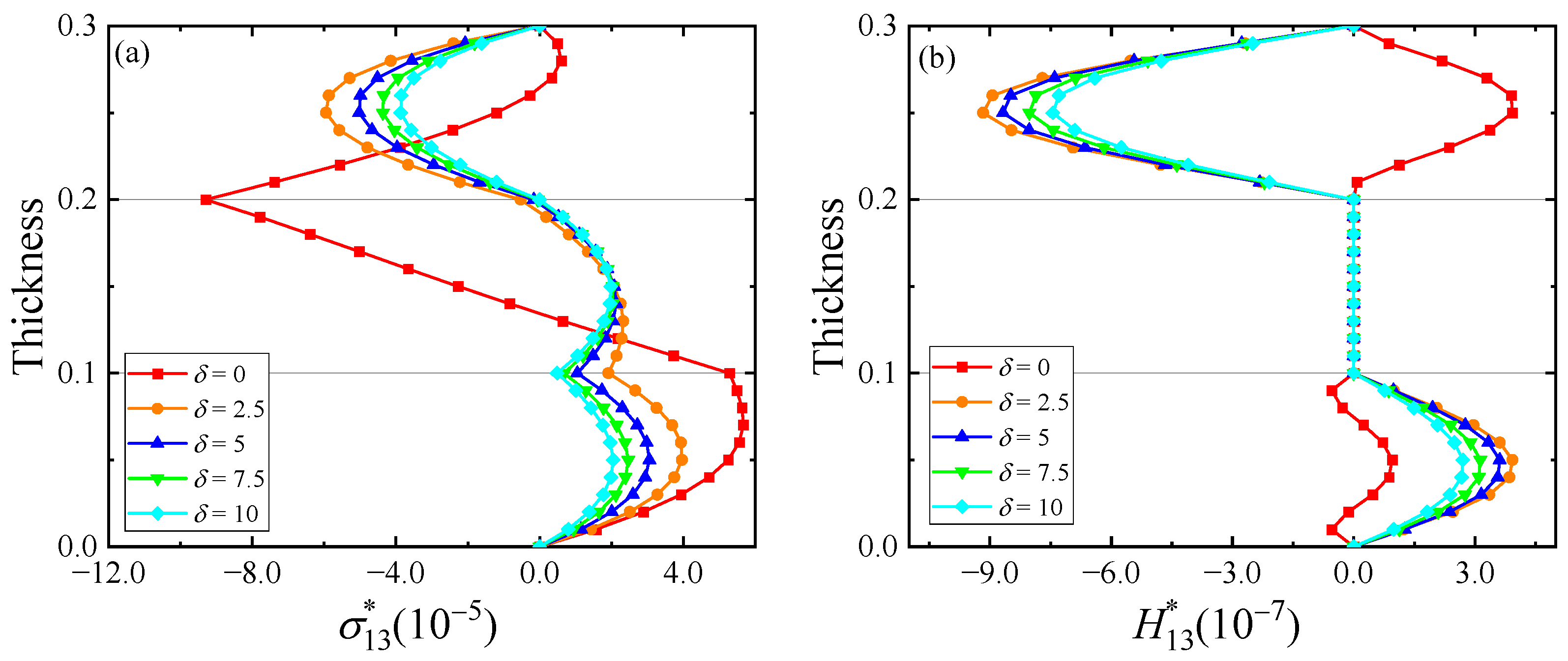
5. Numerical Examples

To validate the accuracy of the proposed method, a numerical example is solved for laminates with simply supported boundary conditions under normal stress (Equation (44)). The geometry and material properties of the plates are taken from the work of Yang et al. [12]. In this analysis, the effect of the electric field is neglected, and the phonon displacement of the laminates along the x₃-direction is determined at the point (x₁, x₂) = (0.75L₁, 0.75L₂). The obtained results are compared with the literature [12] and shown in Figure 2a, demonstrating a high level of consistency. Furthermore, the influence of the number of discrete points on the accuracy of the results is analyzed in Figure 2b. It can be observed that the results tend to converge as the number of discrete points increases, with convergence occurring at N = 7. To ensure the accuracy of the results, a total of 13 discrete points are selected in this study.

This section mainly studies the effect of the interface compliance δ, functional gradient factor η, and initial stress on the static bending of 2D PQC laminates by using the semi-analytical solutions derived in Section 4. To increase computing speed and reduce storage capacity, the dimensionless form of field quantities and frequencies are defined as

$$\begin{array}{l}{u}_i^{*}=\frac{u_i}{L_{\max }}, w_m^{*}=\frac{w_m}{L_{\max }}, {\varphi }^{*}=\frac{\varphi e_{\max }}{L_{\max }{C}_{\max }}, {\sigma }_{ij}^{*}=\frac{{\sigma }_{ij}}{C_{\max }}, H_{mj}^{*}=\frac{H_{mj}}{C_{\max }}, D_i^{*}=\frac{D_i}{e_{\max }}, \\ {\rho }^{*}=\frac{\rho }{{\rho }_{\max }}, {\delta }^{*}=\frac{\alpha \cdot C_{\max }}{R}=\frac{\beta \cdot C_{\max }}{R}=\frac{\gamma \cdot e_{\max }^2}{R\cdot C_{\max }}, \Omega =\omega L_{\max }/\sqrt{{\rho }_{\max }/C_{\max }},\end{array}$$

(43)

where L_max, C_max, e_max, and ρ_max are the maximum values of the side length, phonon elastic coefficients, phonon piezoelectric coefficients, and densities of the 2D PQC laminate, respectively. We assume that the laminate consists of three layers, each with the geometry ratio L₁:L₂:h = 1:1:0.1. The QC material used is Al-Ni-Co alloy, and the crystalline material is BaTiO₃. The parameters of these two materials are given in

Table 1. Material Parameters [39] (C_ij, K_i, R₁ (10⁹ N/m²), e_ij (C/m²), ξ_ii (10⁻⁹ C²/(N∙m²)), ρ (kg/m³)).

	C11	C12	C13	C33	C44	K1	K2	K4
QC1	234.33	57.41	66.63	232.22	70.19	122	24	12
QC2	166	77	78	162	43	0	0	0
	e15	e31	e33	${\xi }_{11}$	${\xi }_{22}$	${\xi }_{33}$	ρ	R1
QC1	5.8	−2.2	9.3	22.4	22.4	25.2	4186	8.846
QC2	11.6	−4.4	18.6	11.2	11.2	12.6	5800	0

, where R₁ = R₂ = R₃ = R₅ = R₆. The discrete points in all examples in this section are taken as N_x = N_y = 13 to meet the computational accuracy and convergence requirements.

Example 1.

Effect of the interface compliance δ* on the static bending of the QC laminates.

We assume that the laminate is homogeneous and that the mechanical load acting on the top surface is

$${\sigma }_{33}={\sigma }_H\sin \left(p{x}_1\right)\sin \left(q{x}_2\right),$$

(44)

where σ_H = −1 N/m².

For fixed (x, y) = (0.25L₁, 0.25L₂), Figure 3 and Figure 4 show the changes in displacements (electric potential) and stresses (electric displacements) along the thickness direction in sandwich QC/Q/QC laminates with SSSS lateral conditions and subjected to mechanical loads. Namely, the top and bottom surfaces of the laminate are, respectively, subjected to tensile pressure. The imperfect interface is dielectrically weakly conducting. When δ* = 0, the interface becomes perfectly connected. It can be seen from Figure 3 that u₁, u_3, and ϕ are continuous when δ* = 0, and the displacement (electric potential) at the interface will undergo a sudden change when δ* ≠ 0. Furthermore, it can be seen from Figure 3a,b that the overall stiffness weakens when δ* rises. The magnitude of w₁ decreases with increasing interface imperfection, indicating that an imperfect interface could affect the local rearrangement of atoms. Figure 4a,b show that a mechanical load would generate a larger stress in the phonon field as compared with the stress in the phason field in Figure 4c. Furthermore, when the imperfect interface factor δ* increases, the maximum magnitude of the stress increases, leading to possible damage to the laminate being easily damaged. Figure 4d shows that the magnitude of the electric displacement D₃ can be very small when considering the effect of the imperfect interface.

We consider now the case of a dielectrically highly conducting interface. Figure 5a–c show the variation of the phonon and phason displacements. By comparing it with the weakly conducting interface (Figure 3), we observe that these displacements are nearly the same, indicating that the dielectric interface condition has nearly no effect, no matter if it is highly or weakly conducting. However, the variations of the electric potential are completely different under different dielectric conditions (Figure 5d vs. Figure 3d). Similarly, while the imperfect interface condition has nearly no effect on the stress, its impact on the electric displacement D₃ is obvious (Figure 6b vs. Figure 4d). For instance, while D₃ is small under weakly conducting conditions (Figure 4d), it is large and increases its magnitude with increasing interface imperfection under the high conduction case.

Example 2.

Effect of the functional gradient factor η on the static bending of the QC laminates.

This section mainly studies the influence of the functional gradient factor on the static bending of CCCC PQC FG laminates under dielectrically weakly conducting conditions. The QC laminate is made of three FG layers, with their pre-exponential properties (i.e., the ones before the exponential factor in Equation (3)) the same as QC/C/QC in Example 1, i.e., with three major layers. In this FG example, each major layer is uniformly divided into ten sublayers. We also assume that while the middle C layer is homogeneous, the top and bottom QC layer is FG with symmetric exponential distribution along the middle C layer. The mechanical load acting on the upper surface is the same as in Example 1 with δ* = 5.

Figure 7 shows the distribution of displacements and electric potential along the thickness direction of FG laminates with different gradient factors. It can be seen from Figure 7 that these quantities vary significantly as η ranges from −0.5 to 0.5. When η = −0.5, the displacements on the top and bottom surfaces reach their maximum magnitude. Notice further that all these field quantities are discontinuous on the interfaces due to the assumed imperfection there. Figure 7d shows the electric potential ϕ has the largest magnitude in the middle layer and its value is more sensitive than those in the top and bottom layers, even though the middle layer is homogeneous. Figure 8 shows the distribution of stress and electric displacement along the thickness direction in FG laminates with different gradient factors. It is observed from Figure 8 that with increasing thickness from the bottom layer surface, the influence of the FG factor η increases. This feature could be related to the fact that the mechanical load is applied on the top surface.

Example 3.

Effect of electric load on the static bending of the QC laminates.

In this example, we assume that an electric load is applied on the top surface of a PQC laminate with a fixed gradient factor η = 0.5 and varying interface compliance δ*. The electric load is the vertical electric displacement assumed as

$$D_{33}=D_H\sin \left(p{x}_1\right)\sin \left(q{x}_2\right),$$

(45)

where D_H = 1 C/m².

Figure 9 and Figure 10 show the variation of displacement (electric potential) and stress (electric displacement) along the thickness direction of the FG QC/C/QC laminate, induced by the surface electric displacement with different interface compliances (dielectrically weakly conducting). It is observed from Figure 9 that the responses under the perfect and imperfect interface conditions are completely different and that the effect of different interface compliances is insignificant. Similar features can be also seen in Figure 10, where the phonon and phason stresses are plotted.

Example 4.

Free and forced vibrations of the QC laminates.

The natural frequency is particularly important for the study of vibration problems. Here we consider SSSS FG PQC laminates made of QC/C/QC with interface imperfection characterized by the interface compliance δ* and functional gradience characterized by the factor η. Similar to Example 2, the middle C layer is homogeneous, and the top/bottom layers are FG with symmetric property distribution with respect to the middle plane of the sandwich laminate.

Table 2. Dimensionless natural frequencies of the sandwich SSSS FG PQC QC/C/QC for different interface compliances δ* and functional gradient factors η.

	δ* = 0	δ* = 2.5	δ* = 5	δ* = 7.5	δ* = 10
η = −0.5	1.3510	0.8549	0.7392	0.6865	0.6560
η = −0.25	1.3563	0.8564	0.7408	0.6883	0.6580
η = 0	1.3616	0.8580	0.7425	0.6902	0.6599
η = 0.25	1.3670	0.8596	0.7442	0.6920	0.6619
η = 0.5	1.3723	0.8612	0.7460	0.6940	0.6639

lists the dimensionless natural frequency for different η and δ*. It is observed from Table 2 that while the natural frequency is insensitive to η (increases slightly with increasing η), it obviously decreases with increasing interface compliance δ*.

We now consider the forced vibration of the same PQC laminate but with fixed η = 0.5, δ* = 5. The mechanical dynamic load applied on the top surface is

$${\sigma }_{33}={\sigma }_H\sin \left(p{x}_1\right)\cos \left(q{x}_2\right)\exp \left(i\omega t\right),$$

(46)

where σ_H = −1 N/m².

Figure 11 shows the variation of the displacements and the eigenmodes along the thickness direction of the sandwich laminate. While Figure 11a,c are for different loading frequencies, Figure 11b,d are the corresponding dimensionless eigenmodes at the fixed dimensionless natural frequency Ω = 0.7460. From Figure 11, the following features can be observed: (1) the displacement variation is roughly antisymmetric with respect to the middle plane of the sandwich; (2) at a fixed thickness value, the magnitude of the displacement increases with increasing loading frequency in the top and bottom layers when the loading frequency is less than the corresponding natural frequency. However, these displacements change their signs when the loading frequency is larger than the natural frequency; (3) the shape of the displacement at Ω = 0.8 is similar to that of the eigenmode in Figure 11b,d.

Figure 12 shows the variation of the stresses along the thickness direction, with Figure 12a,c for different loading frequencies, Figure 11b,d for the corresponding dimensionless eigenmodes at the fixed dimensionless natural frequency Ω = 0.7460. Comparing Figure 12 with Figure 11, we observe that the variation trend for the stresses is similar to that of the displacements. Namely, the three features listed for the displacement apply here for the stress. Similar features can be also seen for the variation of the electric potential and electric displacement along the thickness direction, as shown in Figure 13.

6. Conclusions

In this paper, we have derived the static and dynamic response of a layered FG PQC rectangular laminate with imperfect interfaces. SS-DQM is superior in modeling for QC laminates with clamped or simply supported boundary conditions. Numerical examples are presented to illustrate the impact of the interface compliance, functional gradient factor, and load types on the responses of the QC laminate. The proposed analytical model can be further extended to other QCs or piezoelectric materials. Our parametric studies show the following features:

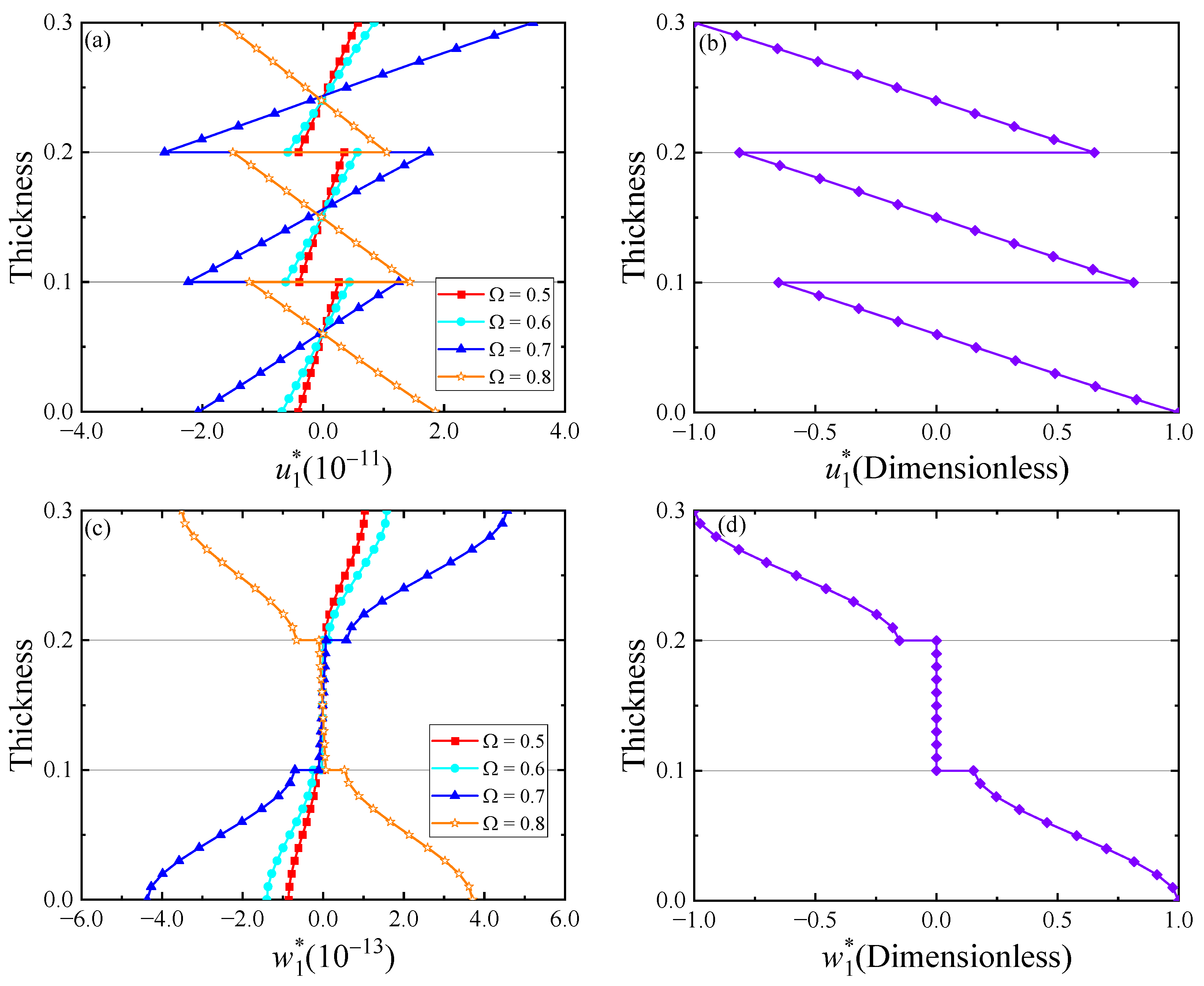
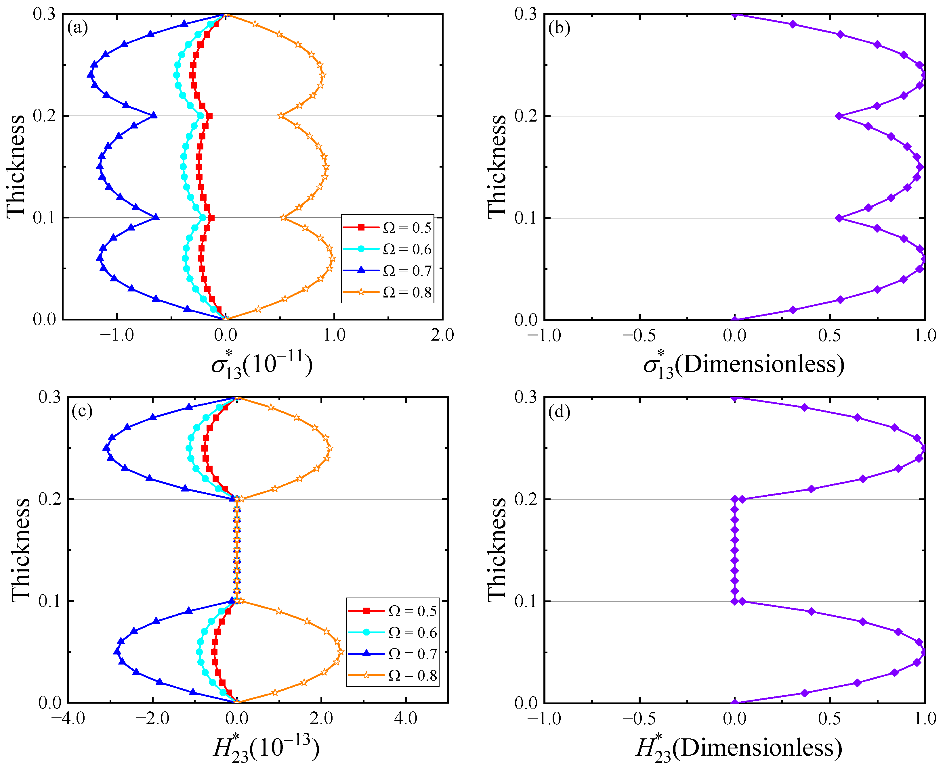
• As the degree of imperfect connection at the interface increases, some physical quantities become discontinuous at the interface, such as displacements.
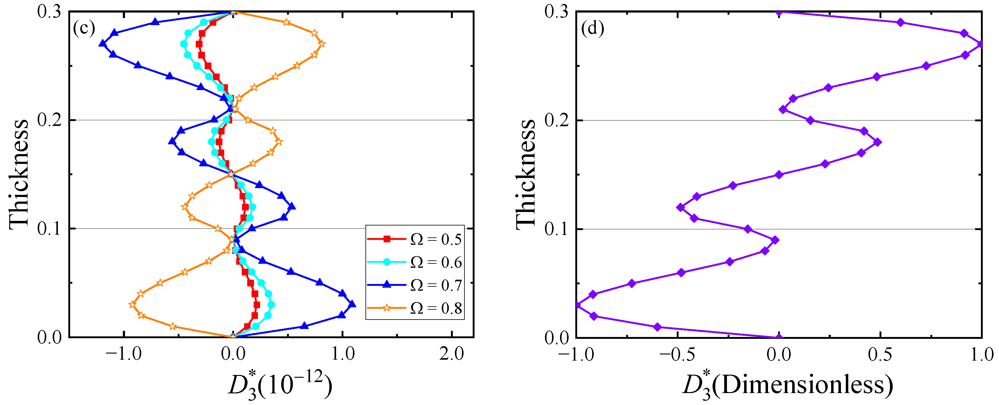
• As the functional gradient factor changes, each physical quantity only changes its numerical magnitude while keeping its variation trend.
• An increase in the interface compliance would reduce the overall stiffness of the laminates while an increase in functional gradient factor would enhance the stiffness. The free vibration frequency will gradually increase as the interface compliance decreases and the functional gradient factor increases.
• The variation trends of the field quantities under different loading frequencies are similar to that of the eigenmode shape at the natural frequency, which is near the loading frequency.

References

1. Shechtman, D.; Blech, I.; Gratias, D.; Cahn, J.W. Metallic phase with long-range orientational order and no translational symmetry. Phys. Rev. Lett. 1984, 53, 1951–1953. [Google Scholar] [CrossRef]
2. Bindi, L.; Steinhardt, P.J.; Yao, N.; Lu, P.J. Natural Quasicrystals. Science 2009, 324, 1306–1309. [Google Scholar] [CrossRef]
3. Bindi, L.; Yao, N.; Lin, C.; Hollister, L.S.; Andronicos, C.L.; Distler, V.V.; Eddy, M.P.; Kostin, A.; Kryachko, V.; MacPherson, G.J.; et al. Natural quasicrystal with decagonal symmetry. Sci. Rep. 2015, 5, 9111. [Google Scholar] [CrossRef]
4. Jaric, M.V.; Nelson, D.R. Introduction to quasicrystals. Phys. Today 1990, 43, 77–79. [Google Scholar] [CrossRef]
5. Fan, T.Y. Mathematical Theory of Elasticity of Quasicrystals and Its Applications; Springer: Heidelberg, Germany, 2011. [Google Scholar]
6. Huang, Y.Z.; Chen, J.; Zhao, M.; Feng, M. Electromechanical coupling characteristics of double-layer piezoelectric quasicrystal actuators. Int. J. Mech. Sci. 2021, 196, 106293. [Google Scholar] [CrossRef]
7. Zhang, L.Y.; Zhang, H.L.; Li, Y.; Wang, J.; Lu, C. Static Electro-Mechanical Response of Axisymmetric One-Dimensional Piezoelectric Quasicrystal Circular Actuator. Materials 2022, 15, 3157. [Google Scholar] [CrossRef] [PubMed]
8. Li, Y.S.; Xiao, T. Free vibration of the one-dimensional piezoelectric quasicrystal microb eams base d on modifie d couple stress theory. Appl. Math. Model. 2021, 96, 733–750. [Google Scholar] [CrossRef]
9. Loboda, V.; Komarov, O.; Bilyi, D.; Lapusta, Y. An analytical approach to the analysis of an electrically permeable interface crack in a 1D piezoelectric quasicrystal. Acta Mech. 2020, 231, 3419–3433. [Google Scholar] [CrossRef]
10. Zhu, S.B.; Tong, Z.Z.; Li, Y.Q.; Sun, J.; Zhou, Z.; Xu, X. Post-buckling of two-dimensional decagonal piezoelectric quasicrystal cylindrical shells under compression. Int. J. Mech. Sci. 2022, 235, 107720. [Google Scholar] [CrossRef]
11. Zhou, Y.B.; Liu, G.T.; Li, L.H. Effect of T-stress on the fracture in an infinite one-dimensional hexagonal piezoelectric quasicrystal with a Griffith crack. Eur. J. Mech. A/Solids 2021, 86, 104184. [Google Scholar] [CrossRef]
12. Yang, L.Z.; Gao, Y.; Pan, E.; Waksmanski, N. An exact solution for a multilayered two-dimensional decagonal quasicrystal plate. Int. J. Solids Struct. 2014, 51, 1737–1749. [Google Scholar] [CrossRef]
13. Guo, J.H.; Zhang, M.; Chen, W.Q.; Zhang, X.Y. Free and forced vibration of layered one-dimensional quasicrystal nanoplates with modified couple-stress effect. Sci. China 2020, 63, 124–125. [Google Scholar] [CrossRef]
14. Huang, Y.Z.; Li, Y.; Zhang, L.L.; Zhang, H.; Gao, Y. Dynamic analysis of a multilayered piezoelectric two-dimensional quasicrystal cylindrical shell filled with compressible fluid using the state-space approach. Acta Mech. 2020, 231, 2351–2368. [Google Scholar] [CrossRef]
15. Huang, B.; Kim, H.S. Free-edge interlaminar stress analysis of piezo-bonded composite laminates under symmetric electric excitation. Int. J. Solids Struct. 2014, 51, 1246–1252. [Google Scholar] [CrossRef]
16. Zhang, L.; Guo, J.H.; Xing, Y.M. Nonlocal analytical solution of functionally graded multilayered one-dimensional hexagonal piezoelectric quasicrystal nanoplates. Acta Mech. 2019, 230, 1781–1810. [Google Scholar] [CrossRef]
17. Vel, S.S.; Batra, R.C. Three-dimensional exact solution for the vibration of functionally graded rectangular plates. J. Sound Vib. 2004, 272, 703–730. [Google Scholar] [CrossRef]
18. Phung-Van, P.; Tran, L.V.; Ferreira, A.J.M.; Nguyen-Xuan, H.; Abdel-Wahab, M. Nonlinear transient isogeometric analysis of smart piezoelectric functionally graded material plates based on generalized shear deformation theory under thermo-electro-mechanical loads. Nonlinear Dyn. 2017, 87, 879–894. [Google Scholar] [CrossRef]
19. Guo, J.H.; Chen, J.Y.; Pan, E. A three-dimensional size-dependent layered model for simply-supported and functionally graded magnetoelectroelastic plates. Acta Mech. Solida Sin. 2018, 31, 652–671. [Google Scholar] [CrossRef]
20. Feng, X.; Zhang, L.L.; Wang, Y.X.; Zhang, J.M.; Zhang, H.; Gao, Y. Static response of functionally graded multilayered two-dimensional quasicrystal plates with mixed boundary conditions. Appl. Math. Mech. 2021, 42, 1599–1618. [Google Scholar] [CrossRef]
21. Ma, W.S.; Liu, F.H.; Li, D.X.; Zhang, J.Y.; Lü, S.F. Global dynamics of a special symmetrically laid composite laminated rectangular plate. J. Inn. Mong. Univ. Technol. 2023, 42, 109–115. [Google Scholar]
22. Benveniste, Y. The effective mechanical behaviour of composite materials with imperfect contact between the constituents. Mech. Mater. 1985, 4, 197–208. [Google Scholar] [CrossRef]
23. Cheng, Z.Q.; Jemah, A.K.; Williams, F.W. Theory for multilayered anisotropic plates with weakened interfaces. J. Appl. Mech. 1996, 63, 1019–1026. [Google Scholar] [CrossRef]
24. Qu, J.M. The effect of slightly weakened interfaces on the overall elastic properties of composite-materials. Mech. Mater. 1993, 14, 269–281. [Google Scholar] [CrossRef]
25. Shariyat, M. A generalized high-order global-local plate theory for nonlinear bending and buckling analyses of imperfect sandwich plates subjected to thermo-mechanical loads. Compos. Struct. 2010, 92, 130–143. [Google Scholar] [CrossRef]
26. Chen, W.Q.; Cai, J.B.; Ye, G.R.; Wang, Y.F. Exact three-dimensional solutions of laminated orthotropic piezoelectric rectangular plates featuring interlaminar bonding imperfections modeled by a general spring layer. Int. J. Solids Struct. 2004, 41, 5247–5263. [Google Scholar] [CrossRef]
27. Bellman, R.; Kashef, B.G.; Casti, J. Differential quadrature: A technique for the rapid solution of nonlinear partial differential equations. J. Comput. Phys. 1972, 10, 40–52. [Google Scholar] [CrossRef]
28. Bert, C.W.; Malik, M. Differential quadrature: A powerful new technique for analysis of composite structures. Compos. Struct. 1997, 39, 179–189. [Google Scholar] [CrossRef]
29. Chen, W.Q.; Lv, C.F.; Bian, Z.G. Free vibration analysis of generally laminated beams via state-space-based differential quadrature. Compos. Struct. 2004, 63, 417–425. [Google Scholar] [CrossRef]
30. Lü, C.F.; Chen, W.Q.; Shao, J.W. Semi-analytical three-dimensional elasticity solutions for generally laminated composite plates. Eur. J. Mech. A/Solids 2008, 27, 899–917. [Google Scholar] [CrossRef]
31. Zhou, Y.Y.; Chen, W.Q.; Lü, C.F. Semi-analytical solution for orthotropic piezoelectric laminates in cylindrical bending with interfacial imperfections. Compos. Struct. 2010, 92, 1009–1018. [Google Scholar] [CrossRef]
32. Lü, C.F.; Lee, Y.Y.; Lim, C.W.; Chen, W.Q. Free vibration of long-span continuous rectangular Kirchhoff plates with internal rigid line supports. J. Sound Vib. 2006, 297, 351–364. [Google Scholar] [CrossRef]
33. Agiasofitou, E.; Lazar, M. On the Constitutive Modelling of Piezoelectric Quasicrystals. Crystals 2023, 13, 1652. [Google Scholar] [CrossRef]
34. Bak, P. Phenomenological theory of icosahedral incommensurate (quasiperiodic) order in Mn-Al alloys. Phys. Rev. Lett. 1985, 54, 1517–1519. [Google Scholar] [CrossRef]
35. Bak, P. Symmetry, stability, and elastic properties of icosahedral incommensurate crystals. Phys. Rev. B 1985, 32, 5764–5772. [Google Scholar] [CrossRef]
36. Lubensky, T.; Ramaswamy, S.; Toner, J. Hydrodynamics of icosahedral quasicrystals. Phys. Rev. B 1985, 32, 7444. [Google Scholar] [CrossRef] [PubMed]
37. Ding, D.H.; Yang, W.G.; Hu, C.Z.; Wang, R.H. Generalized elasticity theory of quasicrystals. Phys. Rev. B Condens. Matter 1993, 48, 7003–7010. [Google Scholar] [CrossRef] [PubMed]
38. Agiasofitou, E.; Lazar, M. On the equations of motion of dislocations in quasicrystals. Mech. Res. Commun. 2014, 57, 27–33. [Google Scholar] [CrossRef]
39. Liu, C.; Feng, X.; Li, Y.; Zhang, L.L.; Gao, Y. Static solution of two-dimensional decagonal piezoelectric quasicrystal laminates with mixed boundary conditions. Mech. Adv. Mater. Struct. 2022, 1–17. [Google Scholar] [CrossRef]
Figure 1. Geometry of a layered QC rectangular laminate with imperfect interfaces.
Crystals 14 00170 g001
Figure 2. (a) Phonon and phason displacement distributions along thickness direction in QC/QC/QC laminate, compared with the results of Ref. [12]. (b) Relative error analysis.
Crystals 14 00170 g002
Figure 3. Variation of the displacements and electric potential along thickness direction in QC/C/QC laminates subjected to mechanical load, under dielectrically weakly conducting conditions with different interface compliances δ*: (a) u 1 * , (b) u 3 * , (c) w 1 * , (d) ϕ * . Coordinates (x, y) = (0.25L1, 0.25L2).
Crystals 14 00170 g003aCrystals 14 00170 g003b
Figure 4. Variation of the stresses and electric displacement along thickness direction in QC/C/QC laminates subjected to mechanical load under dielectrically weakly conducting conditions with different interface compliances δ*: (a) σ 13 * , (b) σ 23 * , (c) H 13 * , (d) D 3 * . Coordinates (x,y) = (0.25L1, 0.25L2).
Crystals 14 00170 g004
Figure 5. Variation of displacements and electric potential along thickness direction in QC/C/QC laminates subjected to mechanical load under dielectrically highly conducting conditions with different interface compliances δ*: (a) u 1 * , (b) u 3 * , (c) w 1 * , (d) ϕ * . Coordinates (x,y) = (0.25L1, 0.25L2).
Crystals 14 00170 g005
Figure 6. Variation of stresses and electric displacement along thickness direction in QC/C/QC laminates subjected to mechanical load under dielectrically highly conducting conditions with different interface compliances δ*: (a) σ 13 * , (b) D 3 * . Coordinates (x,y) = (0.25L1, 0.25L2).
Crystals 14 00170 g006
Figure 7. Variation of displacements and electric potential along thickness direction in FG QC/C/QC laminates subjected to mechanical load, with different functional gradient factors: (a) u 1 * , (b) u 3 * , (c) w 1 * , (d) ϕ * . Coordinates (x,y) = (0.25L1, 0.25L2).
Crystals 14 00170 g007
Figure 8. Variation of stress and electric displacement along thickness direction in FG QC/C/QC laminates subjected to mechanical load, with different functional gradient factors: (a) σ 13 * , (b) H 13 * . Coordinates (x,y) = (0.25L1, 0.25L2).
Crystals 14 00170 g008
Figure 9. Variation of displacement and electric potential along the thickness direction of the FG QC/C/QC laminates under the electric load with different interface compliances δ* (dielectrically weakly conducting) (a) u 1 * , (b) ϕ * . Coordinates (x,y) = (0.25L1, 0.25L2).
Crystals 14 00170 g009
Figure 10. Variation of phonon and phason stresses along the thickness direction of the FG QC/C/QC laminates under the electric load with different interface compliances δ* (dielectrically weakly conducting) (a) σ 13 * , (b) H 13 * . Coordinates (x,y) = (0.25L1, 0.25L2).
Crystals 14 00170 g010
Figure 11. Variation of displacements along the thickness direction of the FG QC/C/QC FG laminates under different loading frequencies (a,c), and dimensionless displacements at the natural frequency Ω = 0.7460 (b,d): (a) u 1 * , (b) u 1 * (natural frequency), (c) w 1 * , (d) w 1 * (natural frequency). Coordinates (x,y) = (0.25L1, 0.25L2).
Crystals 14 00170 g011
Figure 12. Variation of stresses along the thickness direction of the FG QC/C/QC FG laminates under different loading frequencies (a,c), and dimensionless stresses at the natural frequency Ω = 0.7460 (b,d): (a) σ 13 * , (b) σ 13 * (natural frequency), (c) H 23 * , (d) H 23 * (natural frequency). Coordinates (x,y) = (0.25L1, 0.25L2).
Crystals 14 00170 g012
Figure 13. Variation of the electric potential and electric displacement along the thickness direction of the FG QC/C/QC FG laminates under different loading frequencies (a,c), and dimensionless electric potential and electric displacement at the natural frequency Ω = 0.7460 (b,d): (a) ϕ * , (b) ϕ * (natural frequency), (c) D 3 * , (d) D 3 * (natural frequency). Coordinates (x,y) = (0.25L1, 0.25L2).
Crystals 14 00170 g013aCrystals 14 00170 g013b