Article

Mesomechanical Aspects of the Strain-Rate Sensitivity of Armco-Iron Pulled in Tension

1
Laboratory of Mechanics of Heterogeneous Materials, Institute of Strength Physics and Materials Science of the Siberian Branch of the Russian Academy of Sciences, 2/4 Akademicheskii Pr., 634055 Tomsk, Russia
2
Laboratory of Strength Physics, Institute of Strength Physics and Materials Science of the Siberian Branch of the Russian Academy of Sciences, 2/4 Akademicheskii Pr., 634055 Tomsk, Russia
*
Author to whom correspondence should be addressed.
Crystals 2023, 13(6), 866; https://doi.org/10.3390/cryst13060866
Submission received: 18 April 2023 / Revised: 2 May 2023 / Accepted: 7 May 2023 / Published: 25 May 2023

Abstract

:
The phenomenon of the strain-rate sensitivity of metallic materials has been a topic of interest since the first mechanical tests at different strain rates were performed. The problem of its theoretical description appeared simultaneously. Despite the significant number of studies covering this issue, it is necessary to rule out a few drawbacks of previously reported models, which is the goal of this work. Herein, an extension of the elastic–viscoplastic model to a generalized state of stress is proposed while aiming to describe the strain rate sensitivity of Armco-iron samples that were pulled in tension within the framework of the finite-difference method. A mathematical model was formulated using equivalent stress and strain, which alleviated the complexity of the relaxation-type constitutive equations. The critical shear stress (CSS) function describes S-type instability with a single equation. The plastic strain rate was calculated based on the well-known Orowan equation, which is related to dislocation dynamics. In addition, the model took the material’s microstructure into account based on the design of a representative volume element (RVE) using the step-by-step packing (SSP) method. The results of the modeling were compared with the available experimental data and were found to satisfactorily correlate with them. The results suggest that the misfit error between the model and experimental data did not exceed 10% in the range of strain rates under study, which is a reliable outcome.

1. Introduction

Liquid media show practically no resistance to external impacts at low strain rates. For instance, when one immerses their hand in water, no significant resistance is felt. However, if one slaps the water’s surface with one’s palm, some pain will be felt. At high strain rates, liquids develop a resistance or strength that is associated with their viscosity. As for solids, they exhibit an inherent initial strength, even under static loading (at low strain rates). However, according to a large number of experimental works (e.g., [1,2,3,4]), their strength at elevated strain rates can significantly change; generally, it increases with the strain rate. Researchers have been interested in the effect of strain rate sensitivity since the first experiments on it, which are comprehensively reviewed in [2,3]. Lugo et al. [4] reported the results of an experimental study on Armco-iron at different strain rates and temperatures. It was shown that at a constant temperature, the lower yield stress that was observed increased with the strain rate, while the yield stress decreased with an increasing temperature.
Significant progress in solving the problem of plasticity in materials that manifest the yield-point phenomenon was made in the first 25 years after World War II [2]. This also applies to the theoretical description of the strain rate sensitivity of numerous materials. Johnston and Gilman [5] performed an experimental study on the mechanical behavior of LiF and other crystals. They showed that plastic flow is related to dislocation dynamics. The application of this theory gave birth to a class of viscoplastic models, wherein special attention was given to their dislocation density and mobility (e.g., [6,7,8,9,10,11]). The constitutive equations that were formulated allowed the description of the strain rate sensitivity of many materials. For instance, the strain rate sensitivity of several materials that did not demonstrate any Lüders band propagation was successfully described using self-consistent viscoplastic models that implicitly included the materials’ microstructures [9,10,11]. Rida et al. [12] used molecular dynamics (MD) simulations to predict the mechanical behavior of nanocrystalline copper subjected to high strain rates (104–1010 1/s). They argued that increased strain rates give rise to an increase in the deforming stress of up to 2–3 GPa due to delayed dislocation dynamics.
Shioya and Shioiri [8] drew an important conclusion on Lüders banding in iron-based materials. They observed that the inhomogeneous strain distribution in a sample that was subjected to tension was due to the negative-slope stress–strain relation. The so-called “up–down–up” constitutive equation related to the negative-slope stress–strain relation is now widely accepted for describing the yield-point phenomenon, Lüders band propagation, and phase-transition-driven instabilities [13,14,15,16,17,18,19,20,21].
Despite the numerous studies, we believe some aspects have not been fully resolved. To begin with, the shear stress at the point of continuum in the “up–down–up” constitutive equation is specified as a piecewise function (e.g., [14,16,17,20,21]) rather than as a single equation for describing S-type instability. In practice, this drawback is overcome by choosing a segment of the piece-wise function. However, according to Maziere [19] and Yoshida [22], it is more convenient and physically reasonable to have a smooth transition between the negative and positive slopes on the stress–strain curve at the point of continuum [19,22].
Another problem is related to using the theory of unpinning dislocations from the atmospheres of interstitial solute atoms and its modifications [19,23]. This theory provides an interpretation of the mechanism of plastic flow nucleation (in the form of moving shear bands) that is associated with overcoming the potential barriers of solute atoms’ atmospheres. However, describing a material’s strain rate sensitivity within this theory’s framework is impossible since there are no physical reasons for the potential barrier to increase with the strain rate. Therefore, the mechanism of rapid dislocation multiplication is thought to be more reliable than that of unpinning existing dislocations [6]. The use of viscoplastic models is more relevant because they assume a finite rate of defect generation in a loaded solid. These models can explain that the solid needs more time to dissipate the input energy and generate dislocations, which is expressed in an increased stress level on the stress–strain curve at higher strain rates. The only condition for modeling this process is the need to determine the CSS function and the kinetic equation for the plastic strain rate.
Nevertheless, another problem is that there are few studies in which the microstructural features of a certain material are considered in the numerical modeling of Lüders banding [16,21,24]. The inclusion of grain-scale plastic flow in these considerations clarifies the actual mechanism of Lüders band propagation, which is not obvious when modeling the loading of 5–10 cm samples [21].
In this work, we make progress in solving the aforementioned problems and present an extension of the elastic–viscoplastic model to a generalized state of stress taking into consideration grain-scale plastic flow.

2. Material and Methods
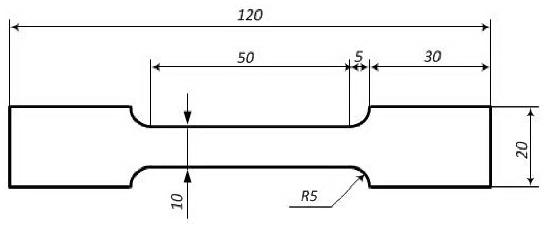
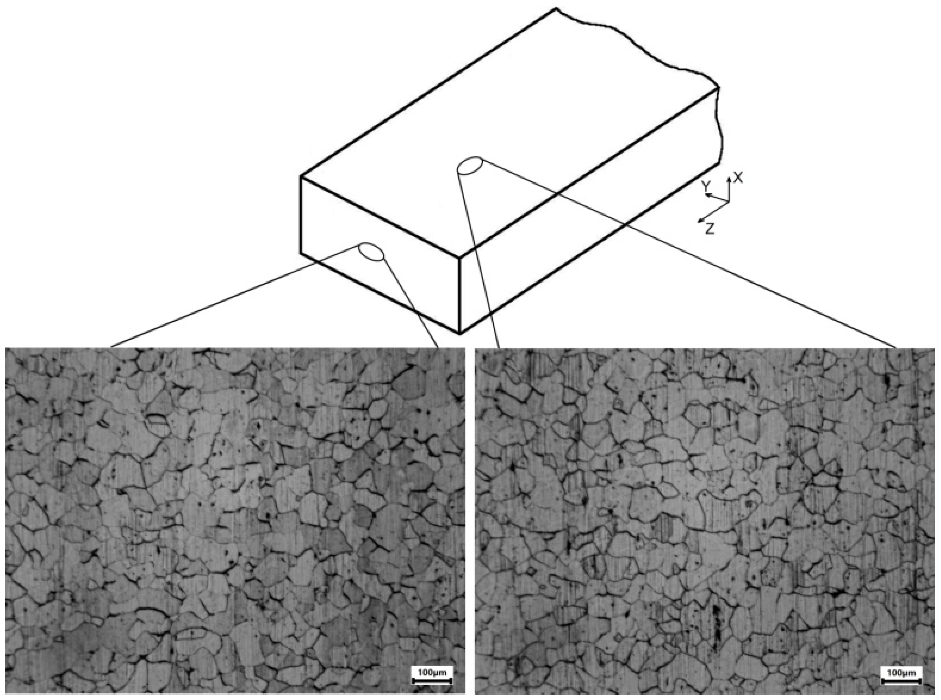
2.1. Material

The experimental material was Armco-iron. Dog-bone tensile test samples (Figure 1) with a gaging section of 50 × 10 × 1.5 mm3 were cut from a cold-rolled sheet using a laser. Then, the samples were annealed at a temperature of 1233 K in vacuum for an hour. The results of a microstructural study were used to obtain the grain size distribution. Based on this study (Figure 2), the grains are spherical without any textural features. The chemical composition of the material is given in Table 1.

2.2. Methods

An S4 Pioneer X-ray fluorescence spectral analyzer was used to determine the chemical composition of the experimental material. A Neophot-21 microscope based on the reflected light optics was used in the microstructural studies. The samples were prepared for the microstructural examination using a standard method [26]. Several abrasives of different grits, M40, M28, M14, and M8, were sequentially applied to grind the samples. ACM 1/0 diamond paste on felt was further used to finish polishing the samples. The microstructure was identified based on the Fe3Cl chemical etching of the samples. An LFM-125 universal testing machine (Walter+Bai AG, Löhningen, Switzerland) with a maximum loading capacity of 125 kN and an accuracy class of 0.5% was used to load the samples. The loading velocity v l varied in the range from 0.02 to 2 mm/min. The samples were pulled in tension without any surface finish. Each experimental point was obtained as an average value from five experiments conducted in the same conditions.
The SSP method [27] with a hand-controlled iteration process was used to design the RVE of Armco-iron. The modeling of the loading of the samples was carried out using in-house software within the framework of a three-dimensional finite-difference method [28] using a workstation with an AMD Threadripper 3990 64-core processor. The scheme for determining the Lüders fronts is given in Figure A3.

3. Mathematical Formulation of the Boundary Value Problem
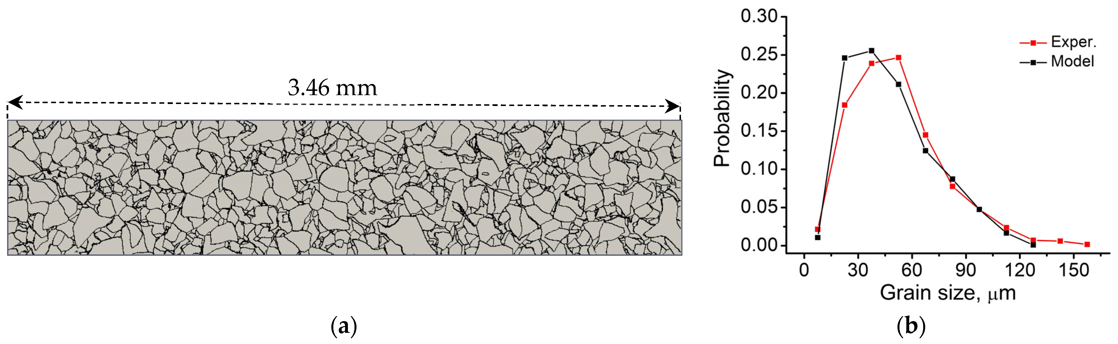
3.1. RVE Design

In this work, we employed the step-by-step packing method that has been proposed elsewhere [27] to design the RVE of polycrystalline Armco-iron. The method is based on a stochastic distribution of the grain nuclei within the computational domain and their step-by-step growth according to a certain law. A spherical fourth-power law was used, and each group of grains (a total of eight groups were considered) was grown separately. (For further details of the RVE design, refer to [21,27].) Figure 3a illustrates the grain distribution in the RVE on the YZ plane. The RVE length was ≈3.5 mm, and the aspect ratio was kept the same as in the experiment. Grains with a size above 130 µm were disregarded in the model due to their insignificant share in the experimental distribution. Figure 3b illustrates a comparison between the experimental and model grain distributions. The mean grain size in the real sample was 52 µm, while that in the model was 48 µm. The mismatch error was approximately 8%. We can conclude that the distributions were in reasonable agreement. The computational mesh contained 1023 × 205 × 31 finite-difference voxels, with a total number of ≈6.5 mln elements. This mesh was chosen as a reasonable trade-off between computational costs and numerical accuracy based on the convergence verification.

3.2. Governing Equations and Elastic Constitutive Response
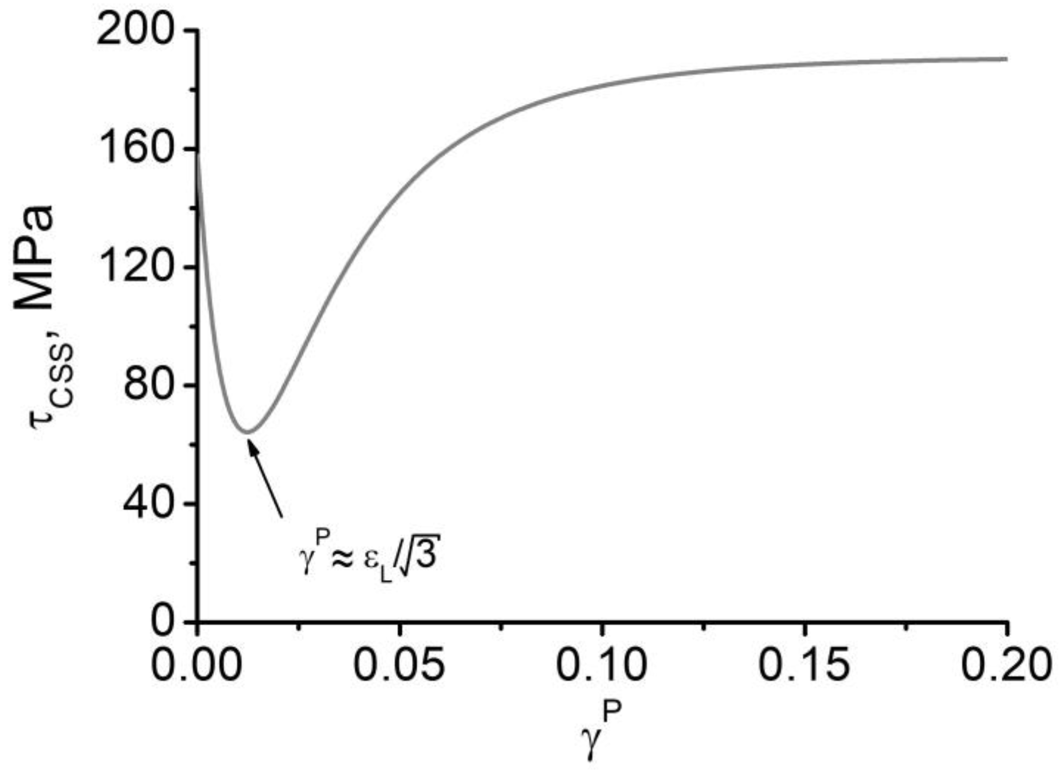
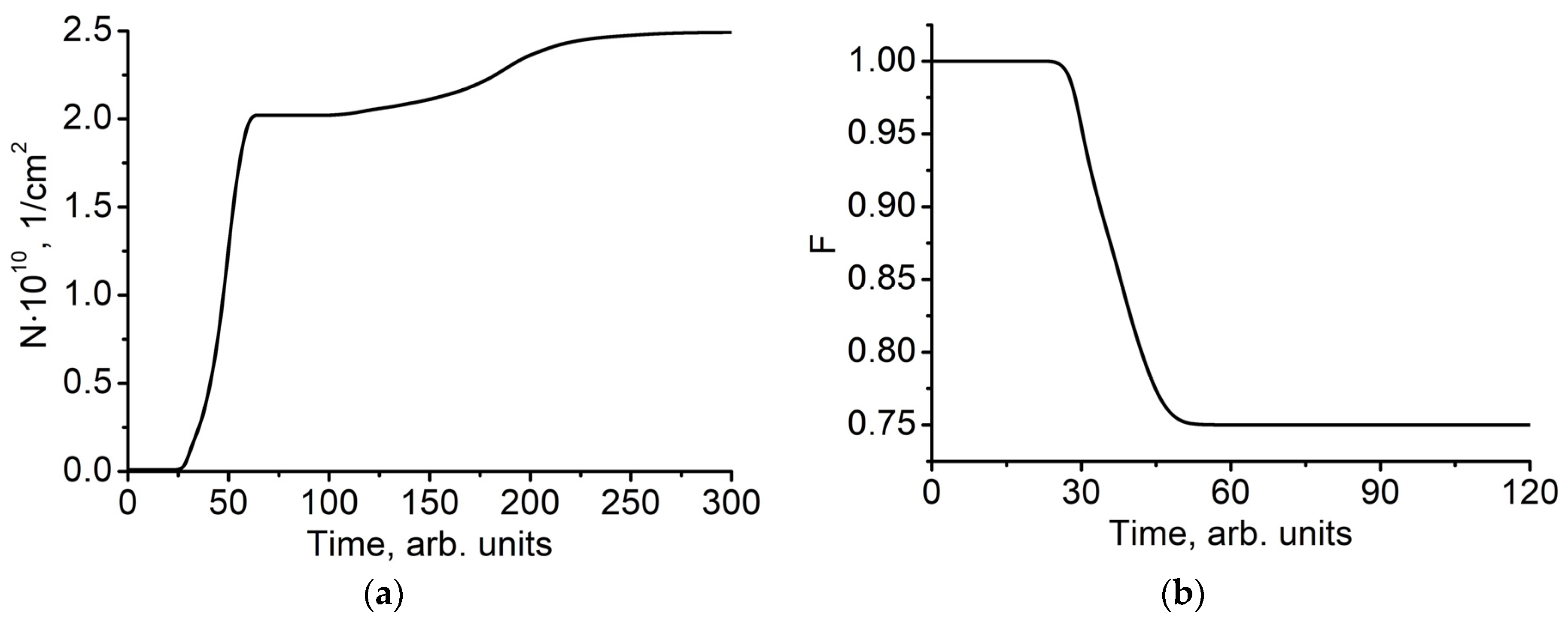
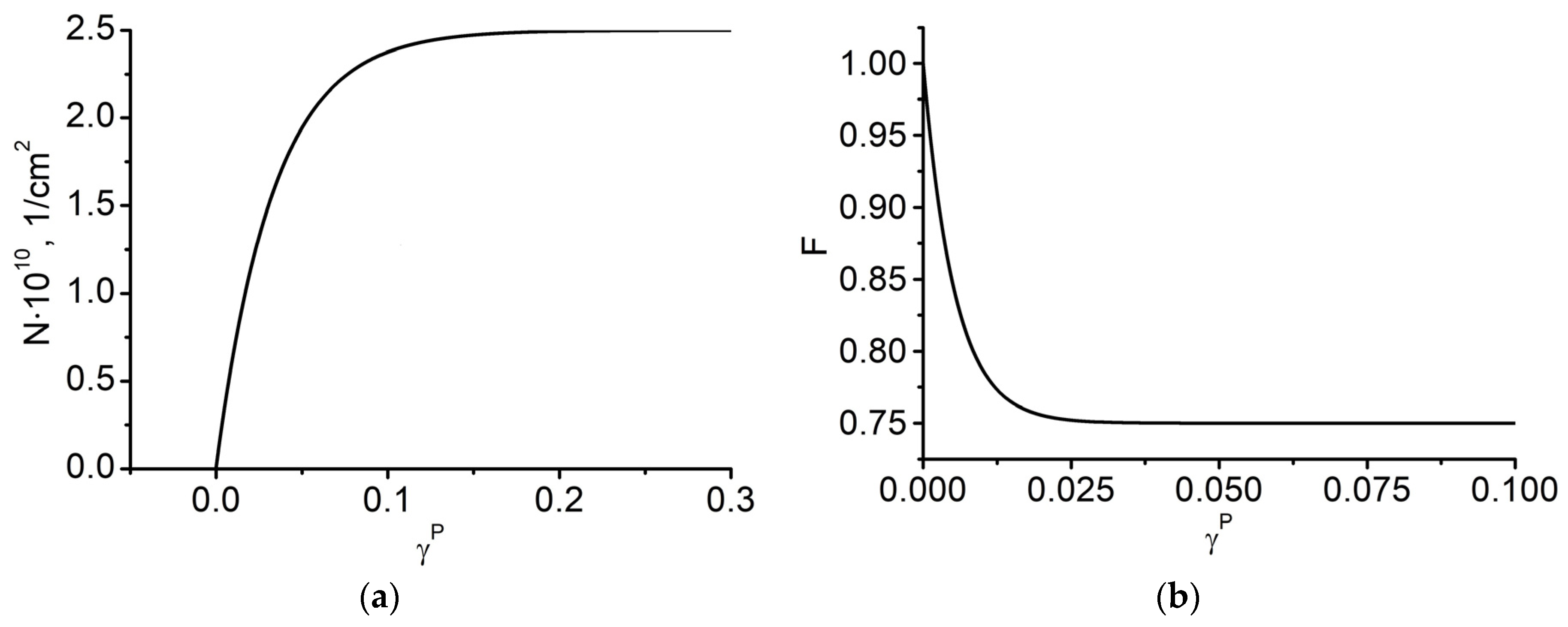
The mathematical model relies on a system of solid mechanics, which is illustrated in Equations (1)–(6) [16,20,21]. The governing equations are derived via the mass (1) and momentum (2) conservation laws:
ρ 0 V 0 = ρ V ,
ρ v ˙ i = σ i j x j ,
where ρ 0 , ρ , V 0 , and V are the density and volume values at the beginning of the deformation process and in the current state, respectively; v i comprises the velocity vector components; σ i j stands for the Cauchy stress tensor components; and x i represents the Cartesian coordinates.
The geometrical relations for the strain rate (Equation (3)) and vorticity (Equation (4)) tensors are also included in the system:
2 ε ˙ i j = v i x j + v j x i
2 ω ˙ i j = v i x j v j x i
We use a relaxation-type constitutive equation of an isotropic medium to calculate the stress increments at each point of the continuum (Equations (5) and (6)). The grains in the RVE are assumed to be isotropic. Therefore, the bulk and shear moduli of the material are easily obtained from the acoustic study. The hydrostatic pressure (Equation (5)) and the deviatoric stresses (Equation (6)) of the Cauchy stress tensor are calculated separately:
P ˙ = K V ˙ V
S ˙ i j + S i k ω ˙ k j S k j ω ˙ i k = 2 μ ε ˙ i j 1 3 V ˙ V δ i j ε ˙ i j P
The Jaumann co-rotation derivative in Equation (6) is used to subtract the rigid rotation of a computational cell that does not influence the values of the deviatoric stress tensor components.

3.3. Plastic Flow

The plastic strain rate is determined using the well-known Orowan equation (Equation (7)), which is related to the mobile dislocation density N m and velocity v , such that
ε ˙ i j P = g N m b v
where g is the orientation multiplier that is generally equal to 0.5 [29] and b is the Burgers vector. Equation (6) assumes that each component of the deviatoric stress tensor relaxes separately over the course of plastic flow development in accordance with Equation (6). This approach is complex; therefore, a simpler approach that is based on the equivalent stress and strain formulation can be employed. In this case, the equivalent stress rate is calculated as follows:
τ ˙ = 3 μ ( γ ˙ T γ ˙ P )
where the equivalent stress τ = 1 2 S i j S i j , and the equivalent plastic strain rate γ ˙ P = 2 3 ε ˙ i j P ε ˙ i j P = 2 3 g N m b v . In the case of a non-zero γ ˙ P value, all components of the deviatoric stress tensor are corrected in the same manner as for the equivalent stress. Otherwise, the equivalent stress continues growing. The ordinary differential Equation (8) is solved numerically with simple iterations within each time step of the numerical integration and each computational cell.
We consider the averaged cooperative contribution from different types of dislocations, which is treated as a dislocation continuum. To calculate the equivalent plastic strain rate in Equation (8), the functions of the mobile dislocations density N m and velocity v need to be determined. Based on the study reported in [8], we used the following functions for the dislocation density N and the fraction of mobile dislocations f :
N = N * + N 0 N * exp   ( A g b γ P )
f = f * + f 0 f * exp   ( B g b γ P )
where N 0 and N * are the initial and limit dislocation densities, respectively; f 0 and f * are the initial and limit fractions of mobile dislocations; constant A stands for the average path of a dislocation until its multiplication; and B stands for the average path of a dislocation until its termination. The density of mobile dislocations N m = N f . A thermodynamics-based justification of the application of this theory is found in [8]. The curves of the dislocation density and the fraction of mobile dislocations at a point of continuum are illustrated in Figure A2a,b, respectively.
An empirical relation for the dislocation velocity is employed [29], which assumes that the dislocation velocity approaches the shear sound speed asymptotically:
v = v 0 q 2 1 + q 2
q = τ e f f β = τ τ C S S β
where v 0 is the shear sound speed, and β is the dislocation deceleration factor, such that its physical meaning is the level of effective stress τ e f f at which the dislocation velocity v asymptotically approaches the shear sound speed. It becomes a non-zero value as soon as τ exceeds τ C S S .
Finally, we have to determine the τ C S S function to describe the plastic flow regularities. In this work, we use the following relation for the critical shear stress:
τ C S S = Y ( γ P ) + k ( γ P ) d 1 / 2
Y γ P = Y 0 + α μ b N
k γ P = k y 1 + 4 γ L γ L + γ P 2 n γ L γ L + γ P n
Figure 4 illustrates the τ C S S at a point in a grain of average size over the course of plastic flow development using Function (12). According to the experimental study performed in this work, the length of the yield plateau or Lüders strain of the sample is ε L ≈ 0.021. The parameters γ L and n are chosen so that the minimum of the τ C S S function is reached when γ P ε L / 3 [21], i.e., when the strain softening is completed and the strain hardening initiates at a point of continuum. Hardening is provided via the change in both Y γ P and k ( γ P ) , which characterize the slip plane stress resistance and the microstructural stress related to the grain-boundary resistance, respectively [30]. Table 2 summarizes the model parameters. The number of model parameters is large in contrast with simpler up–down–up models. However, these parameters have clear physical meanings and interrelate the macroscopic plastic flow with the dislocation dynamics. The determination of the initial values of the Hall–Petch relation parameters is discussed in Appendix A.

3.4. Boundary and Initial Conditions

The following boundary conditions are applied to the model:
(i)
The velocity vector component v z is assigned as v z = v ( t ) and v z = 0 for the upper and the lower supports, respectively;
(ii)
The tangential velocities are v x = 0 and v y = 0 ;
(iii)
The other facets of the sample are free of stress.
Ideal mechanical contact is assumed at the grain junctions. The v ( t ) function increases up to a certain value in the elastic deformation stage and then remains unchanged, which rules out the influence of the acceleration term in Equation (2).

4. Results and Discussion

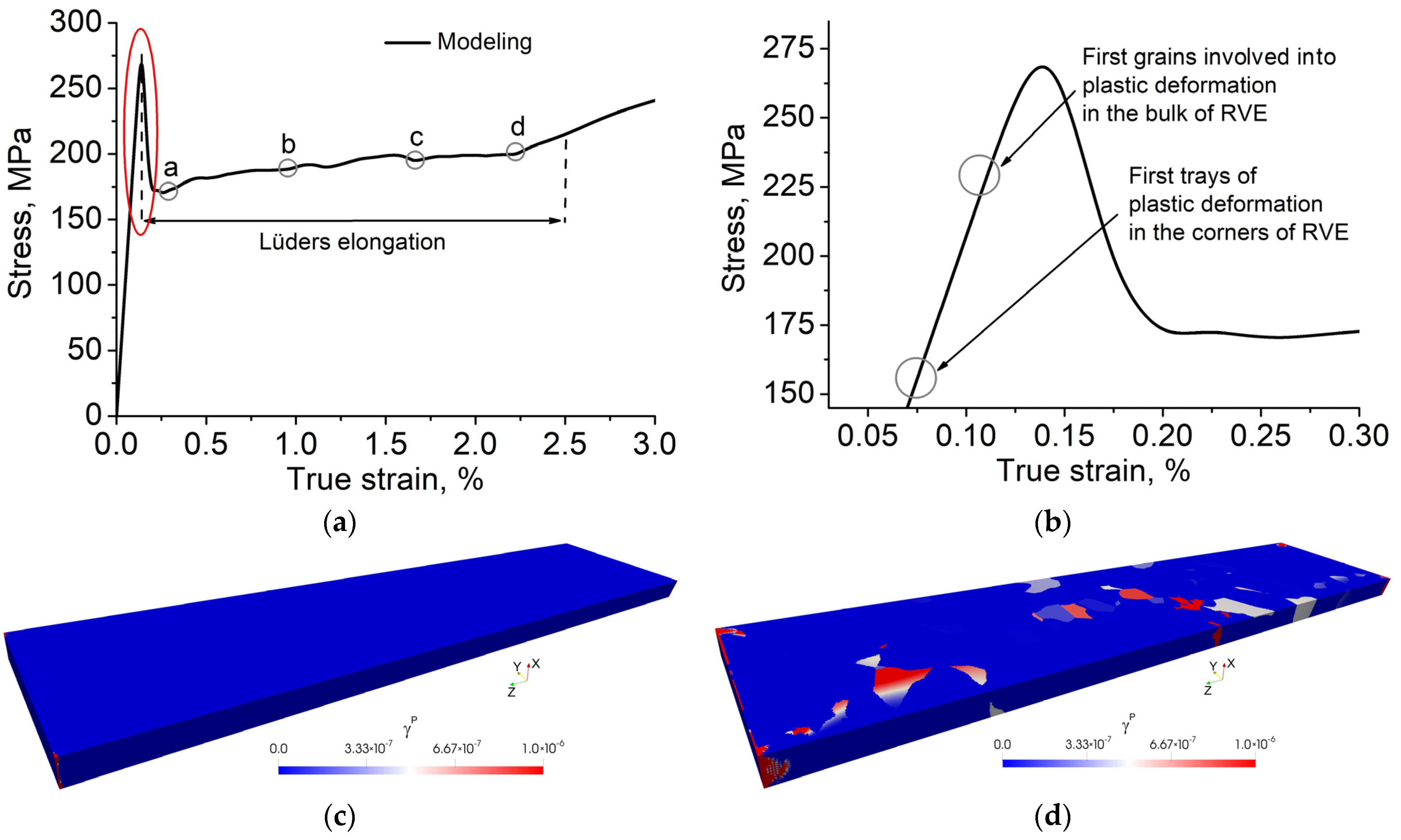
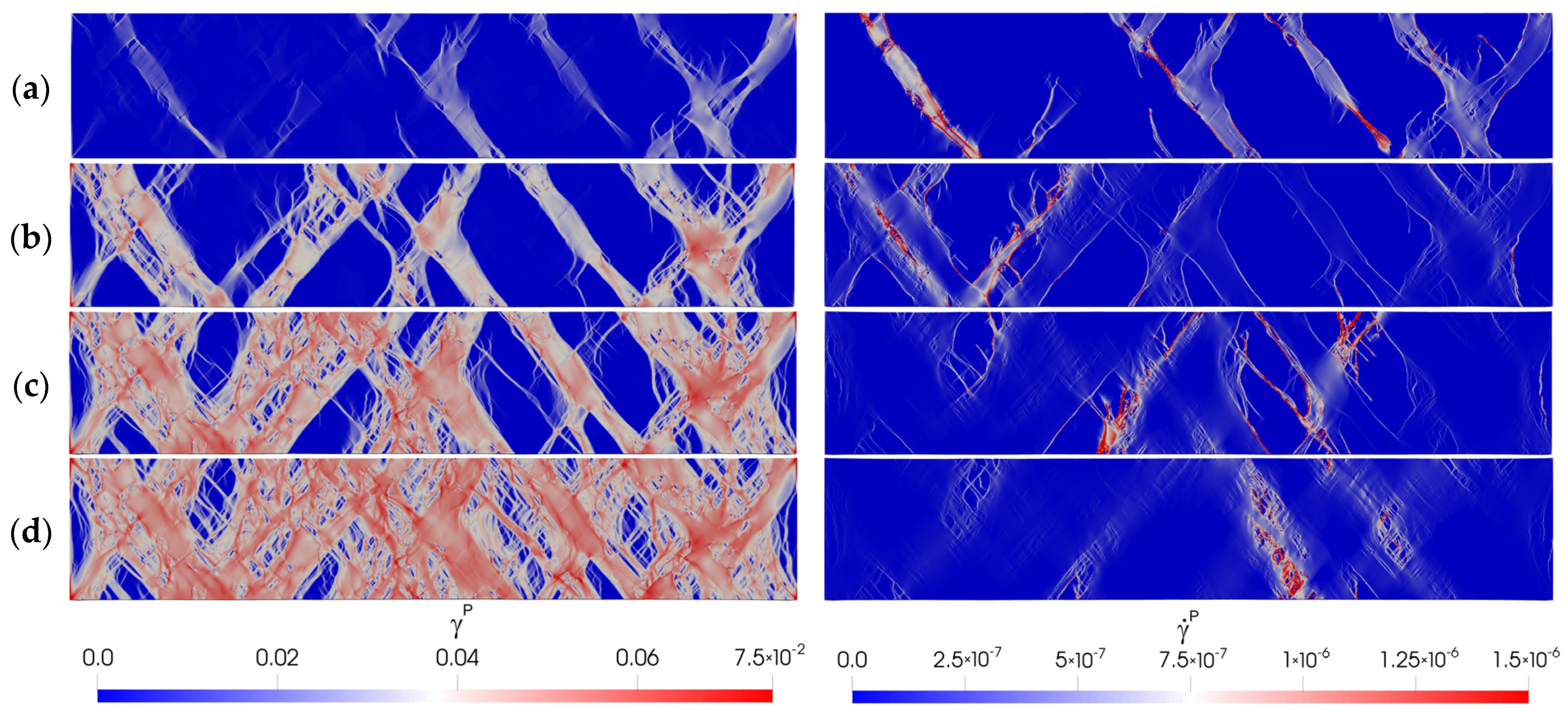
4.1. Features of Plastic Flow at Grain Scale

We will now consider the modeling results. First, we will inspect the patterns of the Lüders front propagation over the mesovolume and compare the stages of propagation with the characteristic states on the flow curve. The stress–strain curve was obtained via the weighted averaging of the stress tensor component σ z z over the entire volume of the computational domain. The macroscopic strain of the sample was calculated as a natural logarithm of the ratio of the current–initial length of the sample.
In this subsection, we analyze the distributions of the plastic strain and plastic strain rates, particularly in the case of a strain rate of ≈3∙10−5 1/s. Then, the kinetic diagram of the plastic flow is constructed using the results of this analysis. Figure 5a shows the mesovolume stress–strain curve in the elastic and yield plateau stages. In addition, Figure 5b illustrates the magnified view of the stress–strain curve at the onset of plastic flow. According to the resulting stress–strain curve, the duration of the yield plateau stage is approximately 2.3%, which slightly exceeds the experimental value (≈2.1%). However, the misfit error in the determination of the yield plateau duration is less than 10%, which is a satisfactory result.
The first traces of plastic deformation due to the stress concentration in the corners of the mesovolume (Figure 5c) appear at an axial stress of approximately 150 MPa, i.e., much earlier than the formation of the effective nucleus of the Lüders front. However, the appearance of traces of plastic deformation does not lead to a noticeable deviation in the averaged flow curve from the elastic law. Figure 5d shows the state of a representative mesovolume when several large grains are involved in the plastic deformation process. The average axial stress, in this case, is approximately 225 MPa, which is ≈20% lower than the observed upper yield stress.
When the axial stress reaches approximately 275 MPa—the observed upper yield stress value—several effective nuclei of Lüders fronts are formed (Figure 6a), which leads to significant stress relaxation. Another behavior of the representative mesovolume is characterized by the propagation of several Lüders fronts as switching waves, transferring the entire computational domain into a plastic state (Figure 6b–d). Qualitatively similar results for low strain rates were obtained in [21,24].
States a–d and the corresponding plastic strain and plastic strain rate distributions are shown in Figure 6a–d. The flow curve demonstrates a gradual increase in the average deforming stress in the yield plateau stage. This is because initially large grains are deformed plastically, and then smaller grains are drawn into the plastic deformation process, which demands a higher deforming stress. Hall et al. [2] and Butler et al. [31] provided an experimental validation of this behavior of Lüders fronts.
Moreover, in state “d” on the flow curve, which is usually characterized by the end of the yield plateau in macroscopic modeling or experiments, not all regions of the representative mesovolume undergo plastic deformation (see Figure 6d). Complete involvement of the computational domain in plastic deformation occurs later, in the stage that macroscopically corresponds to the beginning of the parabolic hardening stage. This feature manifests itself when the grain structure is taken into account and plastic flow is considered at the mesoscale level [21].
A kinetic diagram of the Lüders sub-front propagation is provided in Figure 7. The diagrams are based on the analysis of the plastic strain and strain rate distributions along the central axis in the direction of the RVE loading. According to the data obtained, the yield plateau stage is characterized by the propagation of six to eight sub-fronts moving toward each other and the sample’s ends. The integral velocity of all the sub-fronts averaged over the length of the yield plateau stage satisfies the thumb rule proposed in [31].

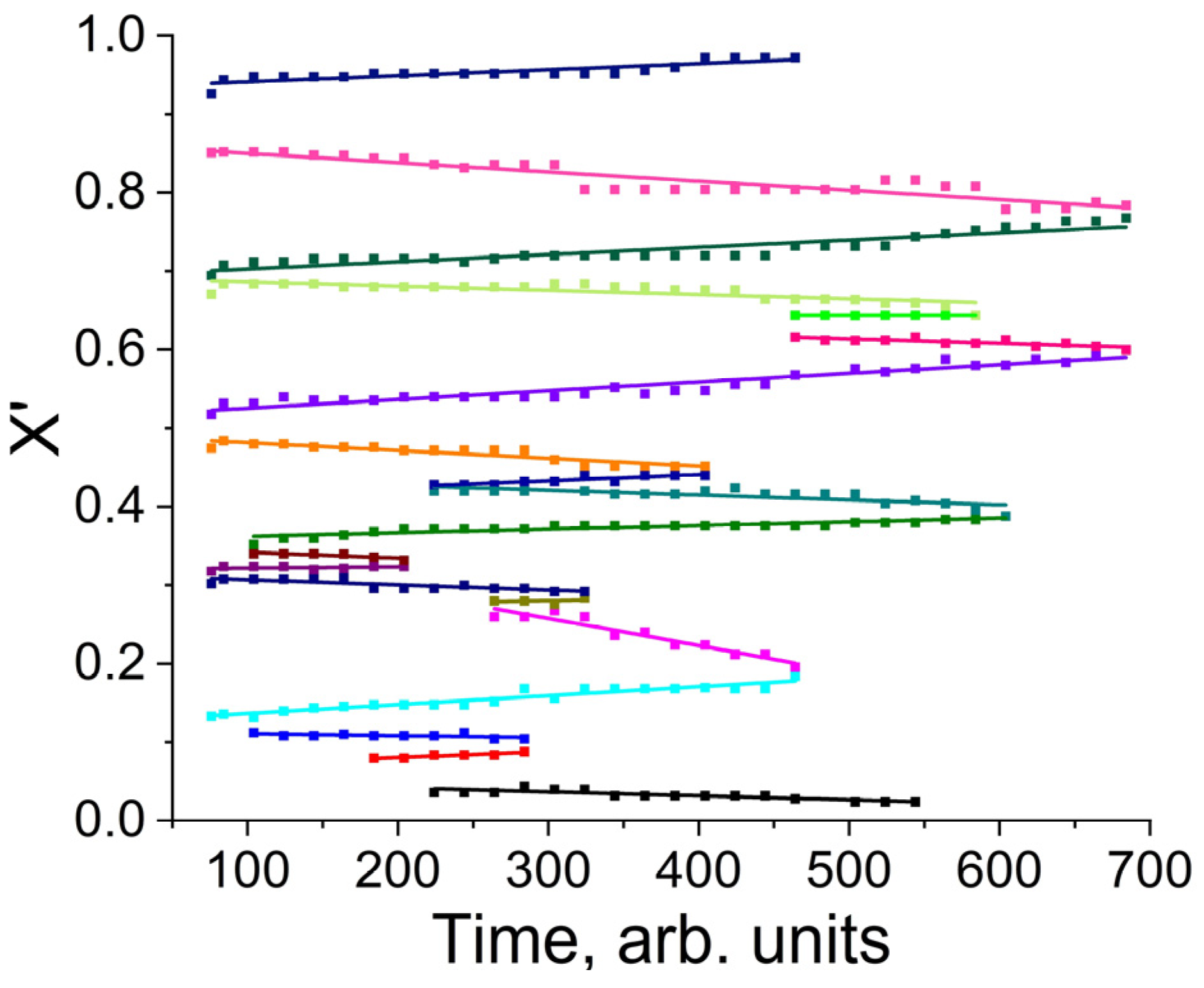
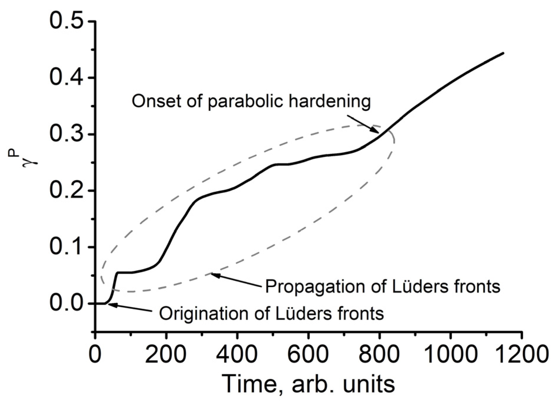
4.2. Features of Plastic Flow at a Point of Continuum

We will now investigate the development of plastic deformation and the corresponding changes in the parameters of the dislocation continuum at one point in the representative mesovolume. According to the modeling data obtained in this work, the dependence of the equivalent plastic strain on time at a point of continuum is a non-linear function. It has some characteristic sections corresponding to different stages, such as the origination and propagation of Lüders sub-fronts and the beginning of the parabolic hardening stage (see Figure 8). Notably, that accumulation of equivalent plastic strain at a point of continuum has a non-monotonic character with periods of acceleration and deceleration at the origination and propagation stage of the Lüders sub-fronts. In particular, the origination of the Lüders sub-fronts (the first segment of the curve) is characterized by the highest rate of increase in the equivalent plastic strain, which correlates in time with significant stress relaxation. The next stage is characterized by several accelerations/decelerations in the growth rate of the equivalent plastic strain.
In contrast with the Lüders sub-front propagation stage, the accumulation of equivalent plastic strain is reasonably smooth in the next parabolic hardening stage of deformation (see the last segment of the curve in Figure 8).
The curves of the dislocation density and the fraction of mobile dislocations (Figure 9a,b) do not significantly change their behavior in the stage-to-stage transition, which is the case in which the equivalent plastic strain is dependent on time. However, these curves behave as logistic functions of time. This indicates that, first, the defect generation process accelerates, and then there is a stable growth stage, which is followed by a slowdown stage.

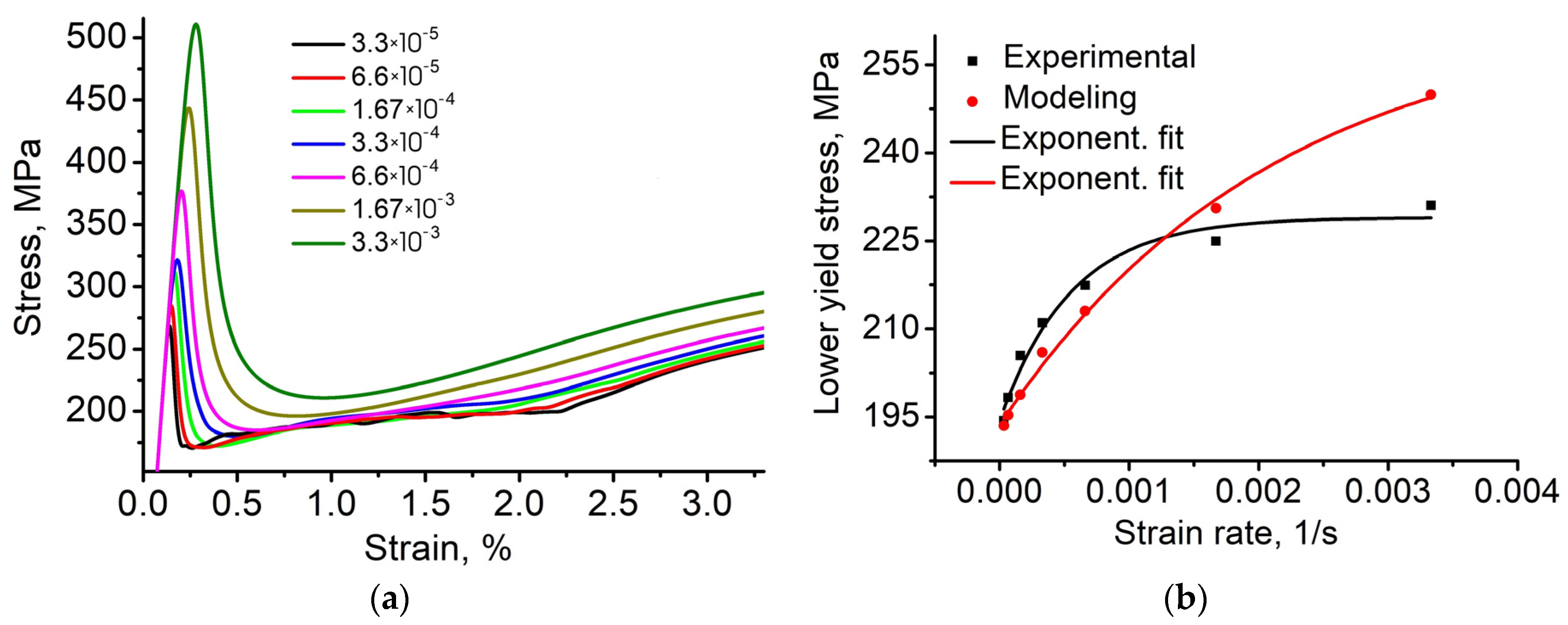
4.3. Strain Rate Sensitivity

The shape of the flow curve in the yield plateau stage indicates that the stress increases as the sub-fronts propagate from the large grains to the small ones. For this reason, we calculated the average stress on the part of the stress–strain curve extending from the observed lower yield stress (the lowest point after the yield tooth) until the computational domain is completely involved in the plastic deformation. For all of the considered strain rates, this process accounts for ≈2.3% of the macroscopic strain.
We will now consider a set of stress–strain curves in the yield plateau stage for different strain rates obtained using numerical modeling (see Figure 10a). It can be seen that the stress–strain curve that was obtained at an increased strain rate lies above the previous one. This implies the results are in reasonable qualitative agreement with previously reported models, e.g., [7,8,12,22]. Moreover, it can be seen that the higher the strain rate, the smoother the stress–strain curve, which is attributed to a not entirely relaxed state, which correlates with the conclusion drawn in [12].
A comparison of the calculated lower yield stress, averaged over the Lüders elongation, with the experimental data obtained in this work is provided in Figure 10b. There is reasonable agreement between the experimental and modeling results for strain rates ranging from 3∙10−5 1/s to 1.67∙10−3 1/s. The misfit error is less than 5%, and for the first two strain rates, the misfit error is even smaller than 2% (see Table 3 for clarity). A further increase in the strain rate results in a more significant deviation in the modeling results from the experimental data. The misfit error increases by almost 10%, which is still reasonable. It is, however, clear that at strain rates higher than 3∙10−3 1/s, the model estimations of the misfit error would exceed 10%.

5. Conclusions

It has been shown that the results of the numerical modeling obtained in this work support the hypothesis that the reason for the strain rate sensitivity of Armco-iron, and probably other materials as well, is due to the limited rate of defect generation in a solid. This results in increased values of deforming stress at higher strain rates.
Taking the microstructure into consideration allowed us to reveal the non-monotonic character of the Lüders sub-front propagation associated with a different grain resistance in the plastic flow. In the case of macroscopic modeling, the actual mechanism of front propagation was not obvious.
A reasonable agreement could be found between the experimental and modeling results in the strain rates ranging from 3∙10−5 1/s to 1.67∙10−3 1/s. The increased model misfit error for strain rates higher than 3∙10−3 1/s suggests that stress relaxation is not adequately described in this range. Therefore, several modifications must be applied regarding the constituents of Equation (7), especially the dislocation velocity. Equation (11) must be modified or replaced with a different empirical relation.
In future work, we plan to include the influence of temperature on the flow stress and the features of the performance of iron alloys in tensile testing.

Author Contributions

Conceptualization, methodology, and writing, M.E.; visualization, software, and formal analysis, A.C.; experimental and formal analysis, V.D. All authors have read and agreed to the published version of the manuscript.

Funding

This work was performed according to the government research assignment for ISPMS SB RAS, project FWRW-2021-0002.

Data Availability Statement

The data are available from the corresponding author upon request.

Acknowledgments

The authors gratefully acknowledge the work of the anonymous reviewers whose critical comments allowed us to improve the manuscript’s quality.

Conflicts of Interest

The authors declare no conflict of interest.

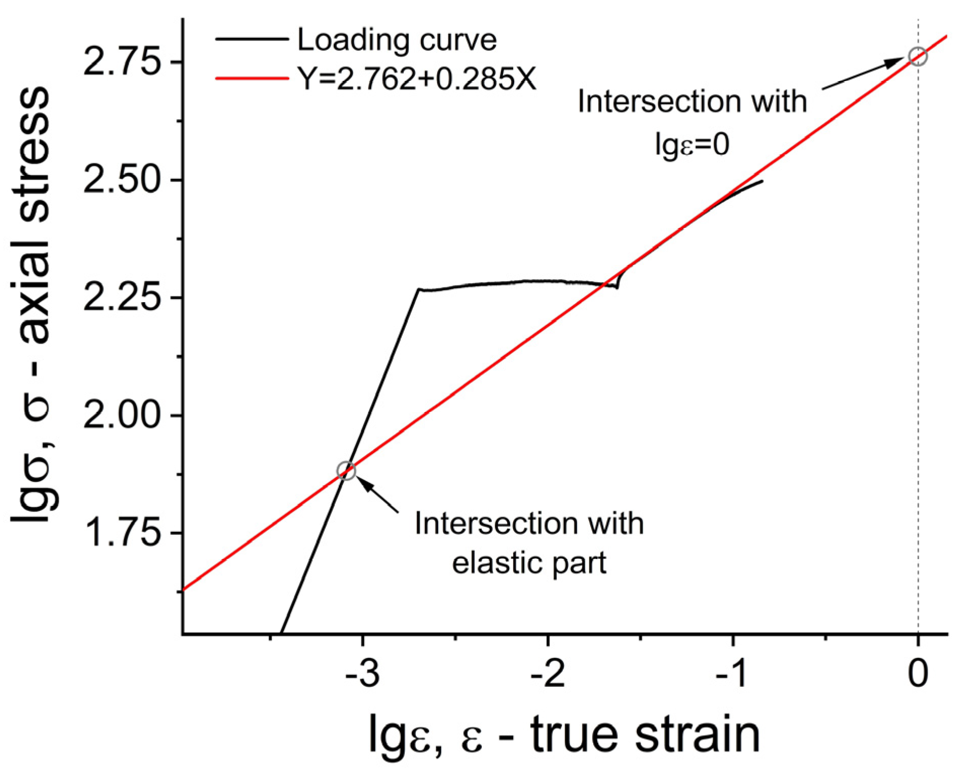
Appendix A. Validation of the Model Parameters

The parameters of the Hall–Petch relation were determined using Rosenfield’s method [32], which is illustrated in Figure A1, wherein the value of σ 0 ≈ 76 MPa (101.88). This value was used in all calculations of Y0 = 44 MPa. An intersection of the linear approximation of the parabolic hardening stage (red line) with lg   ε = 0 gives the value of θ ≈ 578 MPa (102.76), and the hardening exponent n (the slope of the line gives the value of n ≈ 0.285) in the double logarithmic coordinates (Figure A1). Using the relation k y = θ ε L n d 1 / 2 [21], we obtain the value of k y = 1.393 M P a m . An average grain size d is used to calculate the value of k y . An equivalent stress formulation is used in the model. For this reason, the σ 0 and k y parameters are multiplied by the factor 1 / 3 . A detailed discussion of the employed technique is given in [21].
Figure A1. Experimental stress–strain curve of Armco-iron at a strain rate of ≈3∙10−5 1/s plotted logarithmically to show the main points of Rosenfield’s method.
Crystals 13 00866 g0a1
Figure A2. Dislocation density (a) and fraction of mobile dislocations (b) versus the equivalent plastic strain at a point of continuum.
Crystals 13 00866 g0a2
Figure A3. Scheme for determination of the Lüders front position (state “b” in Figure 5 is taken as an example), where the main fronts are marked with red, and the upper and lower patterns correspond to the equivalent plastic strain and plastic strain rate distributions, respectively.
Crystals 13 00866 g0a3

References

  1. Vshivkov, A.; Prokhorov, A.; Uvarov, S.; Plekhov, O. Investigation of mechanical properties of Armco-iron during fatigue test. Mech. Adv. Mater. Mod. Processes 2016, 2, 2. [Google Scholar] [CrossRef]
  2. Hall, E.O. Yield Point Phenomena in Metals and Alloys; Plenum Press: New York, NY, USA, 1970; 296p. [Google Scholar]
  3. Armstrong, R.W.; Walley, S.M. High strain rate properties of metals and alloys. Int. Mater. Rev. 2008, 53, 105–128. [Google Scholar] [CrossRef]
  4. Lugo, N.; Puchi, E.S.; Cabrera, J.M.; Pardo, J.M. Deformation at variable strain rate of ARMCO iron. Rev. Metal. 2004, 40, 139–145. [Google Scholar] [CrossRef]
  5. Johnston, W.G.; Gilman, J.J. Dislocation velocities, dislocation densities, and plastic flow in lithium fluoride crystals. J. Appl. Phys. 1959, 30, 129–144. [Google Scholar] [CrossRef]
  6. Hahn, G.T. A model for yielding with special reference to the yield-point phenomena of iron and related bcc metals. Acta Metall. 1962, 10, 727–738. [Google Scholar] [CrossRef]
  7. Kelly, J.M.; Gillis, P.P. Thermodynamics and dislocation mechanics. J. Frankl. Inst. 1974, 297, 59–74. [Google Scholar] [CrossRef]
  8. Shioya, T.; Shioiri, J. Elastic-plastic analysis of the yield process in mild steel. J. Mech. Phys. Solids 1976, 24, 187–204. [Google Scholar] [CrossRef]
  9. Lebensohn, R.A.; Tomé, C. A self-consistent anisotropic approach for the simulation of plastic deformation and texture development of polycrystals: Application to zirconium alloys. Acta Metall. Mater. 1993, 41, 2611–2624. [Google Scholar] [CrossRef]
  10. Segurado, J.; Lebensohn, R.A.; LLorca, J.; Tomé, C.N. Multiscale modeling of plasticity based on embedding the viscoplastic self-consistent formulation in implicit finite elements. Int. J. Plast. 2012, 28, 124–140. [Google Scholar] [CrossRef]
  11. Galán-López, J.; Shakerifard, B.; Ochoa-Avendaño, J.; Kestens, L.A.I. Advanced Crystal Plasticity Modeling of Multi-Phase Steels: Work-Hardening, Strain Rate Sensitivity and Formability. Appl. Sci. 2021, 11, 6122. [Google Scholar] [CrossRef]
  12. Rida, A.; Micoulaut, M.; Rouhaud, E.; Makke, A. Understanding the strain rate sensitivity of nanocrystalline copper using molecular dynamics simulations. Comput. Mater. Sci. 2020, 172, 109294. [Google Scholar] [CrossRef]
  13. Kubin, L.P.; Estrin, Y. Strain nonuniformities and plastic instabilities. Rev. Phys. Appl. 1988, 23, 573–583. [Google Scholar] [CrossRef]
  14. Shaw, J.A.; Kyriakides, S. Initiation and propagation of localized deformation in elasto-plastic strips under uniaxial tension. Int. J. Plast. 1997, 13, 837–871. [Google Scholar] [CrossRef]
  15. Wenman, M.R.; Chard-Tuckey, P.R. Modelling and experimental characterisation of the luders strain in complex loaded ferritic steel compact tension specimens. Int. J. Plast. 2010, 26, 1013–1028. [Google Scholar] [CrossRef]
  16. Romanova, V.; Balokhonov, R.; Schmauder, S. Three-dimensional analysis of mesoscale deformation phenomena in welded low-carbon steel. Mater. Sci. Eng. A 2011, 528, 5271–5277. [Google Scholar] [CrossRef]
  17. Schwab, R.; Ruff, V. On the nature of the yield point phenomenon. Acta Mater. 2013, 61, 1798–1808. [Google Scholar] [CrossRef]
  18. Hallai, J.F.; Kyriakides, S. Underlying material response for Lüders-like instabilities. Int. J. Plast. 2013, 47, 1–12. [Google Scholar] [CrossRef]
  19. Maziere, M.; Luis, C.; Marais, A.; Forest, S.; Gasperini, M. Experimental and numerical analysis of the Lüders phenomenon in simple shear. Int. J. Solids Struct. 2017, 106–107, 305–314. [Google Scholar] [CrossRef]
  20. Makarov, P.V.; Smolin, I.Y.; Zimina, V.A. The structure of deformation autosoliton fronts in rocks and geomedia. Geodyn. Tectonophys. 2021, 12, 100–111. [Google Scholar] [CrossRef]
  21. Eremin, M.O.; Chirkov, A.O.; Nadezhkin, M.V.; Zuev, L.B. Microstructure-based finite-difference analysis of the plastic flow in low-carbon steel. Eur. J. Mech. A. Solids 2022, 93, 104531. [Google Scholar] [CrossRef]
  22. Yoshida, F.; Kaneda, Y.; Yamamoto, S. A plasticity model describing yield-point phenomena of steels and its application to FE simulation of temper rolling. Int. J. Plast. 2008, 24, 1792–1818. [Google Scholar] [CrossRef]
  23. Cottrell, A.H.; Bilby, B.A. Dislocation theory of yielding and strain ageing of iron. Proc. Phys. Soc. Lond. Sect. A 1949, 62, 49–62. [Google Scholar] [CrossRef]
  24. Mao, B.; Liao, Y. Modeling of luders elongation and work hardening behaviors of ferrite-pearlite dual phase steels under tension. Mech. Mater. 2019, 129, 222–229. [Google Scholar] [CrossRef]
  25. Standard Test Methods for Tension Testing of Metallic Materials. Available online: astm.org (accessed on 30 April 2023).
  26. Beckert, M.; Klemm, H. Handbuch der Metallographischen Atzverfahren; VEB Deutscher Verlag: Leipzig, Germany, 1984; 400p. [Google Scholar]
  27. Romanova, V.A.; Balokhonov, R.R. A method of step-by-step packing and its application in generating 3d microstructures of polycrystalline and composite materials. Eng. Comput. 2019, 37, 241–250. [Google Scholar] [CrossRef]
  28. Wilkins, M.L. Computer Simulation of Dynamic Phenomena; Springer: Berlin/Heidelberg, Germany, 1999. [Google Scholar]
  29. Makarov, P.V.; Romanova, V.A.; Balokhonov, R.R. Plastic deformation behavior of mild steel subjected to ultrasonic treatment. Theor. Appl. Fract. Mech. 1997, 28, 141–146. [Google Scholar] [CrossRef]
  30. Armstrong, R.W. The Dislocation Mechanics of Crystal/Polycrystal Plasticity. Crystals 2022, 12, 1199. [Google Scholar] [CrossRef]
  31. Butler, J.F. Lüders front propagation in low carbon steels. J. Mech. Phys. Solids 1962, 10, 313–318. [Google Scholar] [CrossRef]
  32. Rosenfield, A.R. The significance of σi, the friction stress contribution to the yield point of b.c.c. metals. J. Inst. Met. 1962, 91, 104. [Google Scholar]
Figure 1. Geometry of a dog-bone sample for experimental study. All dimensions are in mm, and the sample thickness is 1.5 mm [25].
Crystals 13 00866 g001
Figure 2. Microstructure of Armco-iron obtained from etched surface on XY (left) and YZ (right) planes after recrystallization.
Crystals 13 00866 g002
Figure 3. Model grain structure on the YZ plane and the RVE size. (a) The aspect ratio of the gage section is the same as in the experiment; (b) a comparison of the experimental and model grain size distributions.
Crystals 13 00866 g003
Figure 4. The τ C S S function at a point in a grain of average size during plastic flow development.
Crystals 13 00866 g004
Figure 5. Stress–strain curve corresponding to the yield plateau stage (a), magnified view of plastic deformation onset stage (b), origination of plastic deformation in the corners of RVE (c), and first yielded grains in the bulk of RVE (d).
Crystals 13 00866 g005
Figure 6. Patterns of plastic strain γ P (left) and plastic strain rate γ ˙ P (right) corresponding to points (ad) on the stress–strain curve. The color legends in Figures (ad) are given at the bottom.
Crystals 13 00866 g006
Figure 7. Kinetic diagram of the Lüders sub-fronts in the yield plateau stage. Different colors correspond to different sub-fronts.
Crystals 13 00866 g007
Figure 8. Equivalent plastic strain versus time at a point of continuum.
Crystals 13 00866 g008
Figure 9. Dislocation continuum parameters versus time: dislocation density (a) and fraction of mobile dislocations (b).
Crystals 13 00866 g009
Figure 10. Set of stress–strain curves in the yield plateau stage for different strain rates obtained using numerical modeling (a) and comparison of the modeling results with the experimental data (the dispersion of experimental data is not illustrated due to its insignificance, at ≤1%) (b).
Crystals 13 00866 g010
Table 1. Chemical composition of Armco-iron (wt. %).
ElementFeCSiMnSPCu
Weight, %The rest0.0250.050.0350.0250.0150.05
Table 2. Summary of model parameters.
ρ 0 , g/cm3 K , GPa μ , GPa N 0 , 1/cm2 N * , 1/cm2 f 0 f *
7.84172791082.5∙101010.75
A g b B g b γ L k y , MPa m Y 0 , MPab 10−8, cmn v 0 , km/s β , GPa α
301900.0850.8532.8663.2340.1
Table 3. Comparison of experimental and modeling results.
Strain Rate, 1/sLower Yield Stress (Exper.), MPaLower Yield Stress (Model.), MPa
3.3∙10−5194.3193.5
6.6∙10−5198.3195.3
1.6∙10−4205.4198.7
3.3∙10−4211205.9
6.6∙10−4217.4213
1.67∙10−3225230.5
3.33∙10−3231249.9
Disclaimer/Publisher’s Note: The statements, opinions and data contained in all publications are solely those of the individual author(s) and contributor(s) and not of MDPI and/or the editor(s). MDPI and/or the editor(s) disclaim responsibility for any injury to people or property resulting from any ideas, methods, instructions or products referred to in the content.

