Modeling Analysis of Melting and Crystallization Process of Mold Flux Based on the Image Processing Technology

Abstract

The aim of this paper is to obtain the image information based on a given image of mold flux and to obtain the features that can describe the dynamical difference. The melting and crystallization dynamics of the slag were analyzed using the autoregressive moving average (ARIMA) time series model and data fitting method. Firstly, the binary image of the digital region of the original image was obtained by image information processing and segmentation methods, the original image number was determined by comparing the similarity of the information matrices of the given and standard images. The standard number with the highest similarity was considered as the number of the original image, and MATLAB was used to solve the problem, the digital information in all the images was successfully extracted. Secondly, ten eigenvalues were extracted from the given image after removing the background, and three principal components were obtained by principal component analysis. Then, a scoring model was constructed based on the percentage of variance, and the comprehensive scores of the three principal components to analyze the melting and crystallization process of the mold flux. Finally, based on the above work, the dynamic relationship between temperature, time and the melting and crystallization process of the mold flux was investigated. Since the temperature is approximately linearly correlated with time, the problem was transformed into finding the relationship between the melting and crystallization process of the mold flux and time. The least squares method, polynomial fitting and other methods were used to derive the relationship function, the relationship between the melting and crystallization process of mold flux and temperature and time was quantitatively analyzed.

1. Introduction

Mold fluxes in the continuous casting process thermally insulate the molten steel meniscus, prevent re-oxidation of liquid steel during continuous casting of liquid steels, control heat transfer, provide strand lubrication and absorb non-metallic inclusions. The metallurgical functions of the mold flux are mainly determined by its melting rate and crystallization rate under the temperature control curve. It is therefore important to study the phase distribution of mold fluxes in the gap between the mold wall and strand shell.

Continuous casting mold fluxes are added to the top of the liquid steel in the mold. These solid slags, which accumulate as a powder layer on the surface of the liquid steel, can prevent the liquid steel level from crusting due to excessive temperature drop of the liquid steel. The temperature of mold fluxes then gradually rises to the melting point, and mold fluxes are melted to form a sintered layer. Raw materials of mold fluxes form low-melting-point substances and then liquid slag through chemical reactions, and the composition of mold fluxes will change to a certain extent. This is the melting process.

When the mold fluxes are completely melted, a layer of liquid slag will form and cover the surface of the molten steel. The slag film is formed when the liquid slag infiltrates from the slag pool on the liquid steel surface into the gap between the shell and the copper mold wall. The slag against the billet is still in the liquid phase due to the high temperature of the billet surface. However, as the temperature of the liquid slag decreases with that of the strand surface in the longitudinal direction of the mold, the slag film, against the copper mold wall, is quenched and solidified to form a glassy solid slag film (solidification behavior of slag film), with the forced cooling, while the slag film will crystallize in certain areas and form a crystalline layer (crystallization behavior of slag film) under suitable conditions, finally forming a typical three-layer slag film structure: glassy layer, crystalline layer and liquid slag layer. This process is called crystallization.

The influence of the mold fluxes on the heat transfer of the mold is mainly realized by the crystalline layer, and the lubricating effect on the steel billet is also influenced by the phase state of the mold fluxes. In general, the lubricating effect of the liquid layer is the best. For the glass layer, premature crystallization or too thick a crystalline layer will affect the lubricating effect. Therefore, it is very important to study the phase distribution of the mold fluxes in the cavity between the mold wall and the solidified blank shell.

Due to the high temperature, transient fluid flow, complex phase transitions and chemical reactions as well as the opacity of the mold wall, it is difficult to directly observe the phase changes of mold fluxes. The single hot thermocouple (SHTT) or double hot thermocouple (DHTT) tester [1] of melting and crystallization temperature testers are now widely used to observe the crystallization behaviors of mold fluxes. After the experiment is completed, the experimenters display the images one by one, record the information in the upper left corner of the images, and identify the key node images by naked eye and experience so as to guide the design of mold fluxes to meet the solidification requirements of steel grades. This process wastes manpower and hinders the development of experimental process information. It is urgent to develop the technology of automatic feature extraction and mathematical modeling of sequence images. Based on the above reasons, this paper has carried out a series of researches on this problem based on image processing technology.

The aim of this paper is to obtain image information based on a given image of mold flux and to obtain the features that can describe the dynamical difference. Through the establishment of a mathematical model, the automatic feature extraction technology of sequence image has been studied, and the functional relationships between the melting and crystallization process of the mold fluxes and the change of temperature, and time have been discussed. The main contributions are as follows:

(1)

The automatic temperature extraction of the thermocouple in each image was realized by using the image segmentation and recognition technologies. By which, it not only reduces the workload of the experimenter, but also reduces the error of visual recognition.

(2)

Based on the collected images, the dynamic difference between the adjacent image sequences in the process of melting and crystallization of the slag was investigated using digital image processing technology. On this basis, the time series modeling of the various characteristics was established and the melting and crystallization curves of the slag were discussed.

(3)

Considering the change of temperature and time, a mathematical model was established to discuss the melting and crystallization kinetics of mold fluxes (the relationship between temperature, melting rate and crystallizing rate).

The remainder of this paper is organized as follows: Section 2 presents the previous work on mold flux crystallization by using DHTT/SHTT technology. Section 3 introduces the data collection process in detail. Section 4 describes the methods used in this paper and the whole process of modeling. Section 5 presents the results obtained. Section 6 discusses the results obtained, concludes the full-text and looks forward to future work.

2. Related Works

It is important to understand the crystallization behavior of these mold fluxes used in the continuous casting of steel because the crystalline phase fraction in the slag films plays a crucial role in determining the horizontal heat flux during the casting process. The existing literature on the crystallization kinetics of conventional and fluoride-free mold fluxes used in the continuous casting of steel has been reviewed by many scientists, such as: Kölbl et al. [2], Sarkar et al. [3] and Wang et al. [4]. Three of the most widely used techniques for studying crystallization kinetics have been included, namely, thermos-analytical techniques such as differential scanning calorimetry/differential thermal analysis (DSC/DTA), single and double hot thermocouple technique (SHTT and DHTT) and confocal laser scanning microscopy (CLSM).

With the help of SHTT and DHTT, the crystallization processes of mold fluxes for metallic materials have been extensively investigated. In the research of Zhou et al. [5], the casting of low-carbon (LC) and medium-carbon (MC) steels was investigated by using DHTT. The crystallization behavior of CaO-SiO₂- and CaO-Al₂O₃-based mold fluxes for casting high-alloy steels was investigated by using SHTT and scanning electron microscope, and kinetic models were developed [6,7].

In addition, small additions of different materials can significantly alter the melting temperature and viscosity of a mold flux. In order to compensate for the negative effect caused by the absorption of chromium oxide inclusions during the casting process of Cr-containing steels, a new mold flux system was designed and investigated by Wang et al. [8]. An investigation aimed at improving the crystallization property of lime-alumina-based fluxes for casting high Al-bearing steels was carried out by Lu and Wang [9] by studying the effects of fluorine and BaO on the crystallization behaviors of the mold flux. The effect of MnO content on the contact angle and interfacial tension between liquid mold flux and ultra-low carbon steel was also investigated by the sessile drop method [10]. In the paper by Liu et al. [11], the SHTT, X-ray diffraction and back scattered electron (BSE) were used to study the crystallization behavior in terms of continuous cooling transformation (CCT) and time temperature transformation (TTT) diagrams of mold fluxes with high Li₂O content. In the papers by Zhou et al., the heat transfer properties of mold fluxes with different amounts of Al₂O₃ [12,13] and B₂O₃ [14] were studied, respectively. In the study by Yang et al. [15], the crystallization behavior and heat transfer of CaO-SiO₂-Na₂O-B₂O₃-TiO₂-Al₂O₃-MgO-Li₂O fluorine-free mold fluxes with different Na₂O contents (5 to11 mass pct) were investigated using SHTT/DHTT and the infrared emitter technique (IET), respectively. A series of slags with the CaO/SiO₂ ratio of 1.1 and different Al₂O₃ contents were designed by Sun et al. [16]. The variation of slag properties during cooling processes, including crystallization ability and glass forming ability, were investigated using SHTT and the results showed that the variation of Al₂O₃ content greatly changed the slag properties, which had a great effect on the heat recovery of slags. In the paper by Yang et al. [17], the crystallization behavior of a mold flux using SHTT/DHTT and the crystallization behavior of CaO-SiO₂-Na₂O-B₂O₃-TiO₂-Al₂O₃-MgO-Li₂O fluorine-free mold fluxes with different CaO/SiO₂ ratio technique were also investigated [18].

In addition to SHTT and DHTT, new optical microscopes and optical processing software systems have also been developed to investigate problems associated with crystallization. A modified apparatus was designed by Kölbl et al. [19] which avoids some of the disadvantages of the previously used apparatus, such as: a rectangular slag film of uniform thickness often cannot be achieved, the minimum temperature often lies within the slag film and so on. In addition, three promising mold slag compositions containing the selected oxides were designed and characterized by Kölbl [20] in the laboratory using a furnace crystallization test, mineralogical investigations and the SHTT/DHTT. In the work of Li et al., the complete crystallization process of the mold flux in the crucible was successfully recorded in situ using a digital optical microscope and image processing software in an infrared furnace (IR-MOP) [21]; the relationship between the crystallization and the breakage temperature of the mold flux was also investigated [22]. The in situ crystallization behavior of high volatile commercial mold fluxes for medium carbon steels has been investigated using the CLSM, the high volatile compounds of the mold flux were suppressed during heating [23].

Although there is a lot of research in this field, most of the literature discusses the effect of different additives to improve the crystallization properties of protective slag. However, there are few examples in the literature that use digital image processing technology to study the dynamic differences between adjacent images in the melting and crystallization process of mold flux, and to characterize these differences quantitatively, so as to study the relationship between temperature, time changes and the melting and crystallization progress of the mold flux. Based on this, this paper mainly focuses on the application of digital image processing technology in the melting crystallization process of the mold flux. The image processing method was used to extract features, time series modeling was established and the melting crystallization process of the mold flux was studied.

3. Data Acquisition

As mentioned above, in the actual continuous casting process, due to the high temperature in the mold, transient fluid flow, a variety of complex phase transitions and chemical reactions, as well as the opacity of the mold wall, it is difficult to directly observe the phase changes of the mold fluxes. In this study, a SHTT Ⅱ melt crystallization temperature tester is used to observe the crystallization process and obtain relevant data, all data used in this article are provided by the Asia and Pacific Mathematical Contest in Modeling. A photo of the SHTT Ⅱ experimental equipment is shown in Figure 1 [24].

The experimental procedure is as follows:

(1)

Thirty grams of decarbonized mold flux are ground with a particle size of 200 mesh, and the 2–3 mg ground sample is placed on the contact point of the thermocouple; the temperature is continuously raised to 1500 °C. During this process, the mold flux gradually melts from solid to liquid.

(2)

The temperature of the liquid protection slag is maintained for 30 s, and then the slag sample is cooled at a cooling rate of 50 °C/s. During the cooling process, the crystal changes in the slag pool are observed in situ. Meanwhile, crystals are gradually precipitated. The dehydration temperature at different heating rates and the time of start and end of crystallization during cooling were recorded.

(3)

In the process of cooling to room temperature, the image analysis software of the visual interface was used to observe the mold flux in the slag pool, and it was confirmed that the experiment was over when the slag pool was completely solidified.

The images of the slag melt crystallization process at different times are shown in Figure 2.

The 6 images in Figure 2 correspond to the six physical change nodes in the sequence image of the molten crystallization process of the mold fluxes. In the above experimental process, an image is generated every second, and the duration of each group of experiments is about 700 s. The accumulation of dynamic differences between adjacent images is the melting and crystallization process of the slag.

However, in this process, the experimenter usually only pays attention to the time and temperature curves corresponding to the six nodes and ignores a large amount of process information, resulting in the vast majority of effective information being ignored and not exploited to its potential.

In addition, the device itself has the privacy protection of its own intellectual property, the time and temperature corresponding to each image cannot be automatically obtained. Only after the experiment can the key node image be identified by opening the images one by one, and recording the information in the top left-hand corner of the image, separately. This process wastes a lot of manpower and is an obstacle to the further development of experimental process information.

The data used in this paper are the sequence images of the melting and crystallization process of the mold fluxes. These sequence images are collected from the 110th to 671st second of the start of the experiment. The file serial numbers follow the collection time sequence, and images are collected every 1 s. The information is presented as digital images. In the upper left corner of each image, the corresponding time of the image and the temperature values of thermocouple No. 1 and No. 2 are marked.

4. Methods

4.1. Extraction of Temperature Information

For the automatic extraction of temperature information, this paper adopts the method of converting color RGB (red, green and blue) image into grey value and then converting it into a binary image to obtain the digital information in the image. In a color RGB image, each pixel contains R, G and B information. Generally, the weighted sum of R, G and B is used as the calculation method of grey value, namely:

$$gra{y}_{ij}=0.299\times R_{ij}+0.587\times G_{ij}+0.114\times B_{ij}$$

(1)

where, grey_ij is the greyscale value corresponding to the pixel in column j of row i after the operation; R_ij, G_ij and B_ij represent the RGB information corresponding to the pixel in column j of row i before the operation, respectively. After obtaining the corresponding grey value of the pixel in row i and column j, the threshold value is used to solve the corresponding binary graph of the pixel at that point, namely:

$$b{w}_{ij}=U(gra{y}_{ij}-t_s)$$

(2)

where bw_ij is the binarization result corresponding to the pixel in row i and column j after the operation, and t_s is the threshold in the binarization process. U is the unit step function. If the independent variable of the function is greater than or equal to 0, the value of the function is 1, and if the value of the function is less than 0, the value of the function is 0. Then the final binarization result can be expressed as the following matrix:

$$bw=\left|\begin{array}{cccccc}b{w}_{11}& b{w}_{12}& \dots & b{w}_{1j}& \dots & b{w}_{1n}\\ b{w}_{21}& b{w}_{22}& \dots & b{w}_{2j}& \dots & b{w}_{2n}\\ \dots & \dots & \dots & \dots & \dots & \dots \\ b{w}_{i1}& b{w}_{i2}& \dots & b{w}_{ij}& \dots & b{w}_{in}\\ \dots & \dots & \dots & \dots & \dots & \dots \\ b{w}_{m1}& b{w}_{m2}& \dots & b{w}_{mj}& \dots & b{w}_{mn}\end{array}\right|$$

(3)

In the matrix above, b_w is the matrix representing the final digital information. An information matrix can be determined by comparing it with the information matrix of each standard number. To determine the information matrix with digital information, the difference between the information obtained and the standard digital information can be compared by comparing its two-dimensional correlation coefficient with the standard digital image:

$$r=\frac{{\displaystyle \sum _i{\displaystyle \sum _j\left(b{w}_{ij}-\overline{bw}\right)}}\left({b{w}^{\prime }}_{ij}-\overline{b{w}^{\prime }}\right)}{\sqrt{\left({{\displaystyle \sum _i{\displaystyle \sum _j\left(b{w}_{ij}-\overline{bw}\right)}}}^2\right)\left({\displaystyle \sum _i{\displaystyle \sum _j{\left(b{w_{ij}}^{\prime }-\overline{b{w}^{\prime }}\right)}^2}}\right)}}$$

(4)

where r is the two-dimensional correlation coefficient between the digital information matrix and the standard digital information matrix. bw′_ij is the element in row i, column j of the standard numerical information matrix. The greater r, the closer the numeric information matrix is to the standard numeric information matrix. For ten Arabic numerals, the following methods can be used to determine which digital information is contained in the matrix.

$$R=\max \left(r_0,r_1,\dots ,r_9\right)$$

(5)

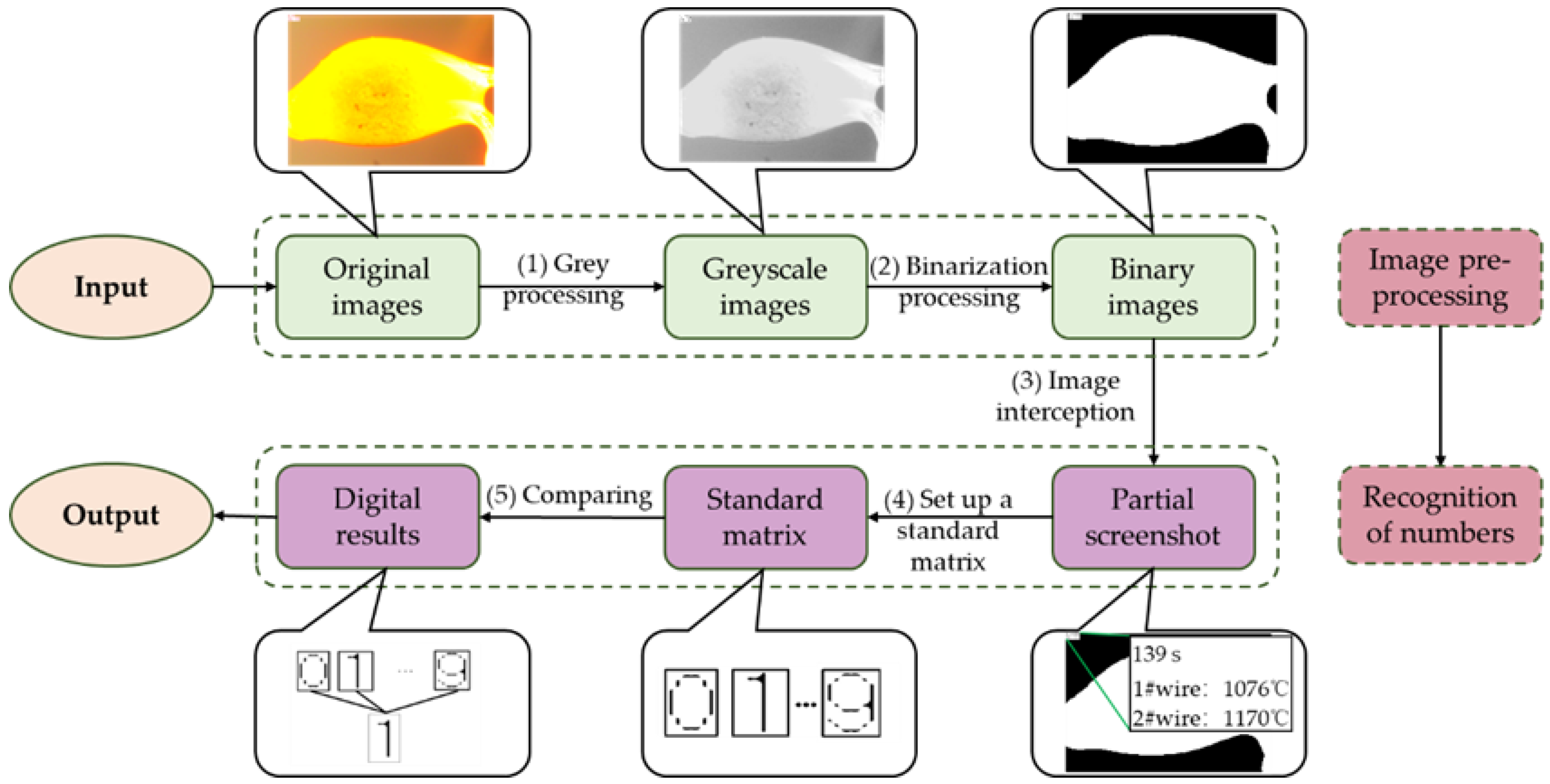
where r₀, r₁,…, r₉ represent the two-dimensional correlation coefficient between the matrix containing the information of a certain number and the matrix containing the information of nine Arabic numbers. R represents the maximum of the two-dimensional correlation coefficient between the matrix of a given number and the matrix of the binary information of each Arabic numeral. The standard number corresponding to the maximum value can be considered as the digital information contained in the information matrix. The above process can be described in Figure 3.

As shown in Figure 3, for a given image, the temperature information in the upper left corner of the image can be read as follows: (1) Greyscale processing: calculate the greyscale value of each pixel by using the weighted sum of R, G and B as the greyscale value, and return the digital image after greyscale value processing. The enlarged figure contains the digital information after grey value processing. (2) Binarization processing: by setting a threshold of 0.5, the greyscale image can be converted into a binary graph, return the processed binary image. The enlarged part shows the digital information after binarization. (3) Image interception: in order to improve the efficiency and the accuracy of judgment, the digital part must be intercepted. By comparing the digital information of the image with the model, the matrix of binarization digital information can be obtained. (4) Set up a standard matrix: since the digital information contained in the matrix is affected by the font of the number, in order to obtain the number consistent with the font in the figure, ten Arabic numerals are manually selected from the image, a matrix containing the information of the ten numbers is established. (5) Comparing and determining the information: compare the obtained matrix of the numbers with the standard matrix of the ten Arabic numerals using a two-dimensional correlation coefficient, the temperature information can be automatically determined by using the value of the two-dimensional correlation coefficient.

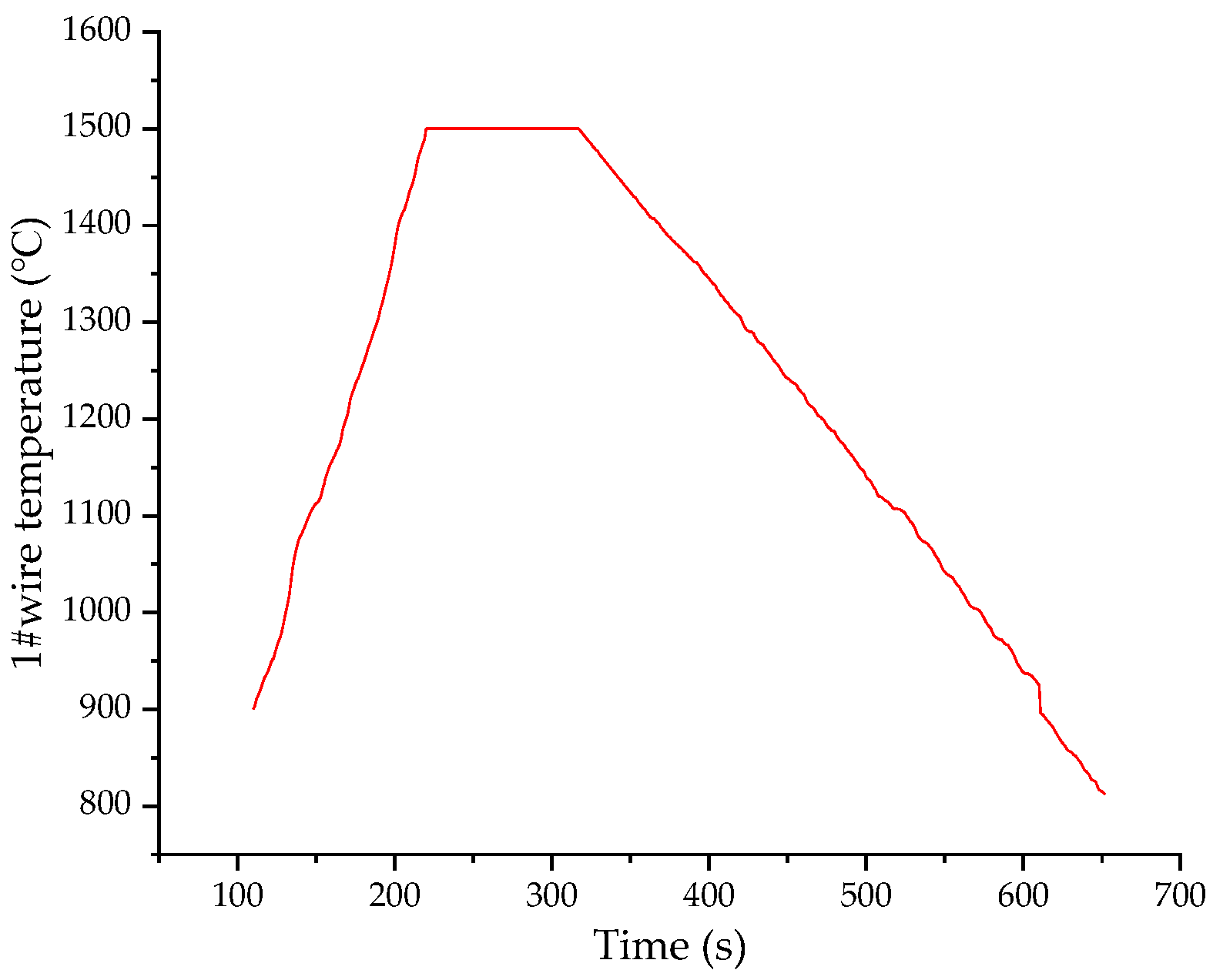
Figure 4 shows the variation of the thermocouple temperature over time obtained by the image processing method.

As shown in Figure 4, the red solid line represents the curve of the temperature measured by the thermocouple over time. It can clearly be seen that as the time changes from 110 to 220 s, the temperature increases approximately linearly with time. When the time reaches 220 s, the measured temperature remains stable at 1500 °C (this is the upper limit of the SHTT-type melting temperature tester). When the time reaches 317 s, the temperature starts to decrease and the cooling rate remains basically constant during the cooling process. Finally, the measured temperature of the thermocouple reaches about 812 °C.

To ensure that the information obtained is from the slag, the images used in the following steps were removed from the background, which effectively reduces the background interference of the image and improves the accuracy of the model solution to some extent.

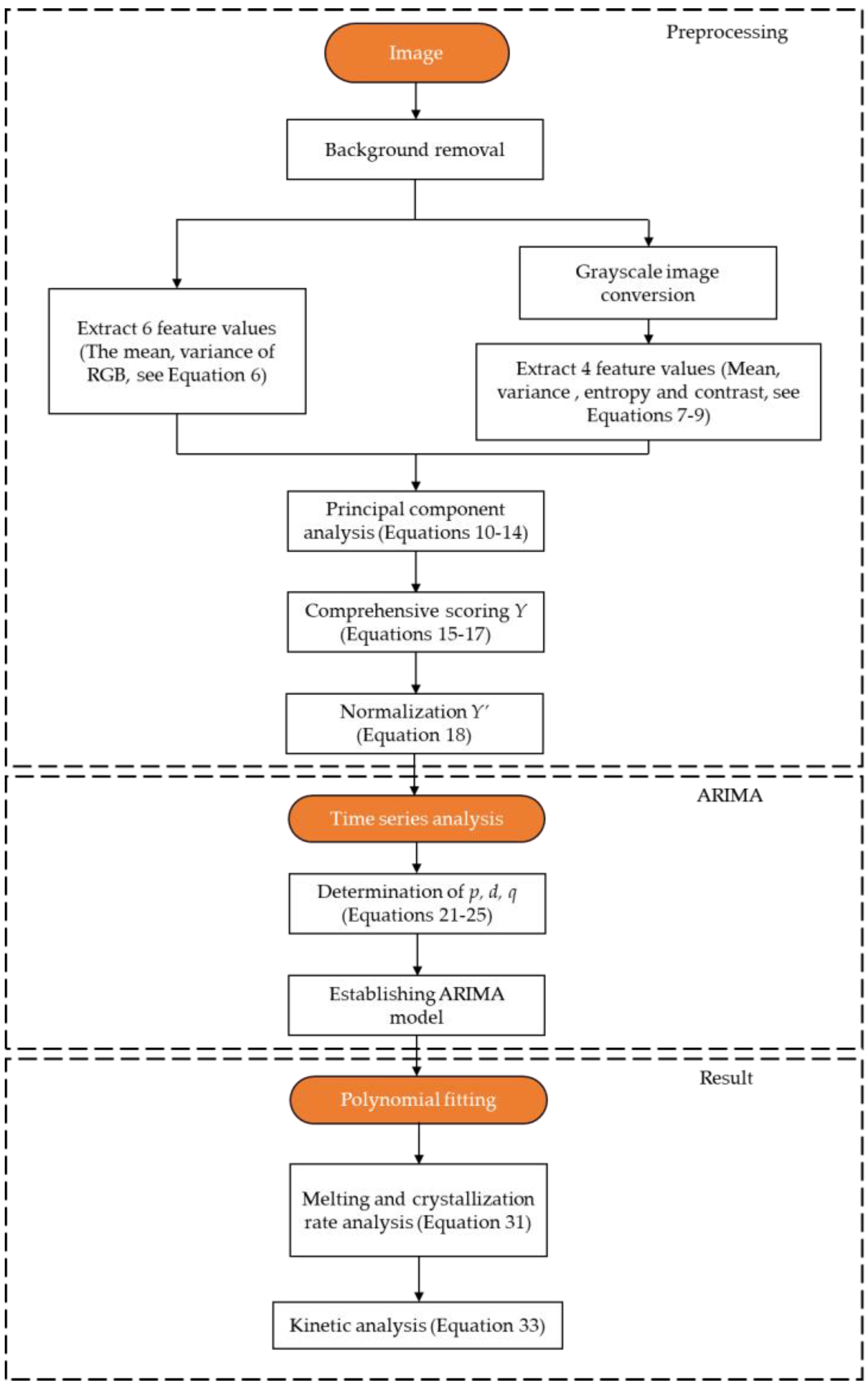
4.2. Extraction of the Image Feature Information

For this problem, the first thing to do is to obtain as many features as possible in the image. These features mainly include color momentum, grey mean value, energy and entropy, and so on. Using the information obtained, time series modeling is carried out using statistical methods. In addition, a special discussion is required for six node images to assess the validity of the selected features.

The image features can be divided into color features, shape features, grey features and edge features, and so on [25]. However, the shape change and edge features are not obvious for the melting image of mold flux investigated in this paper, which are not considered. The color and grey features are mainly studied. Color features are quantified and analyzed mainly by means of the mean and variance of image RGB, the grey features are analyzed mainly by mean and variance of the grey image, entropy and contrast.

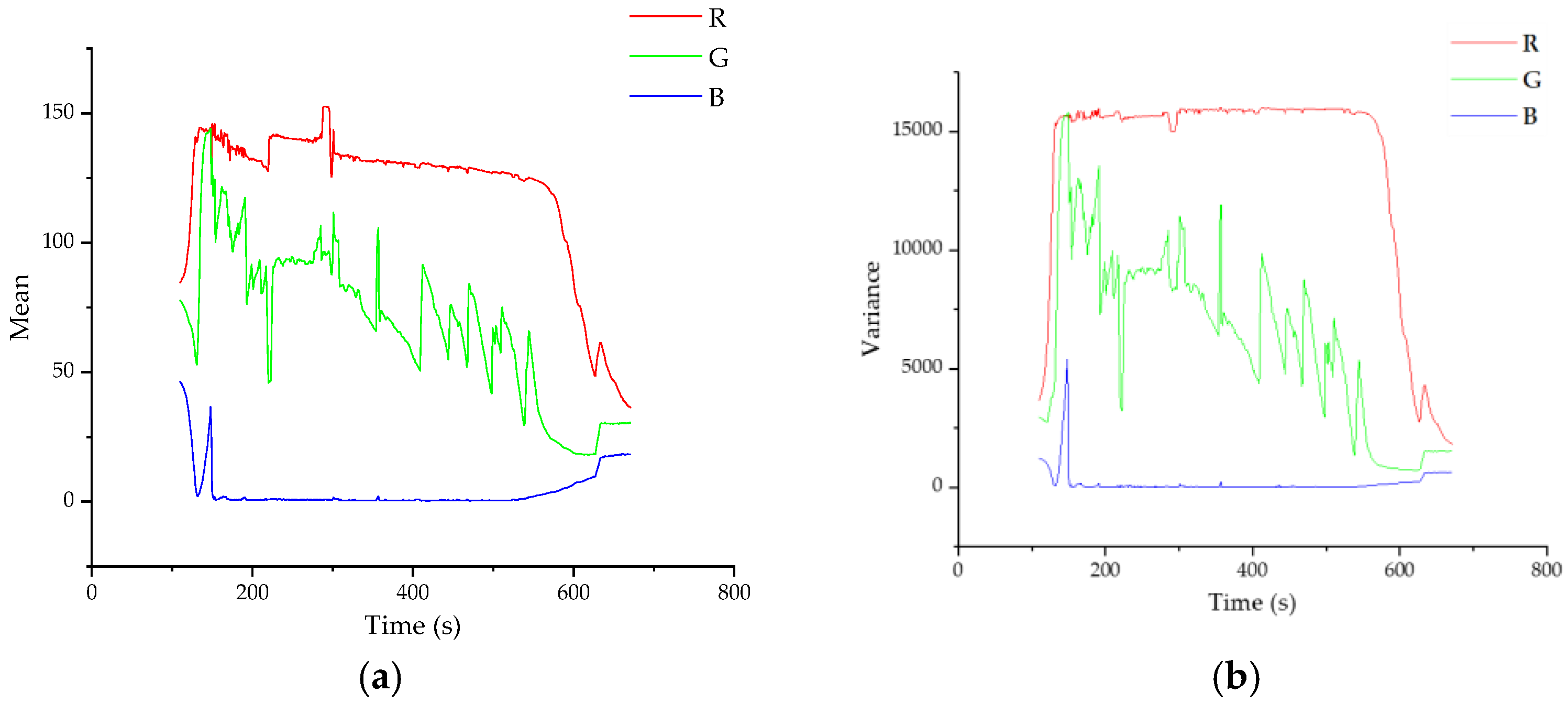
4.2.1. Extraction of Color Moment Features

For a color image in the RGB color space, the three-dimensional color moment is the mean value, variance and slope of the three-color components:

$$\{\begin{array}{l}{\mu }_n=\frac{1}{N}{\displaystyle \sum _i^N{n}_i}\\ {\sigma }_n=\sqrt{\frac{1}{N}{\displaystyle \sum _{i=1}^N{(n_i-{\mu }_n)}^2}}\end{array} (n=R,G,B)$$

(6)

where μ_n and σ_n represent the mean and variance of the three-color components, respectively. n_i represents the value of the color component n at the i-th pixel. N is the total number of pixels in the image.

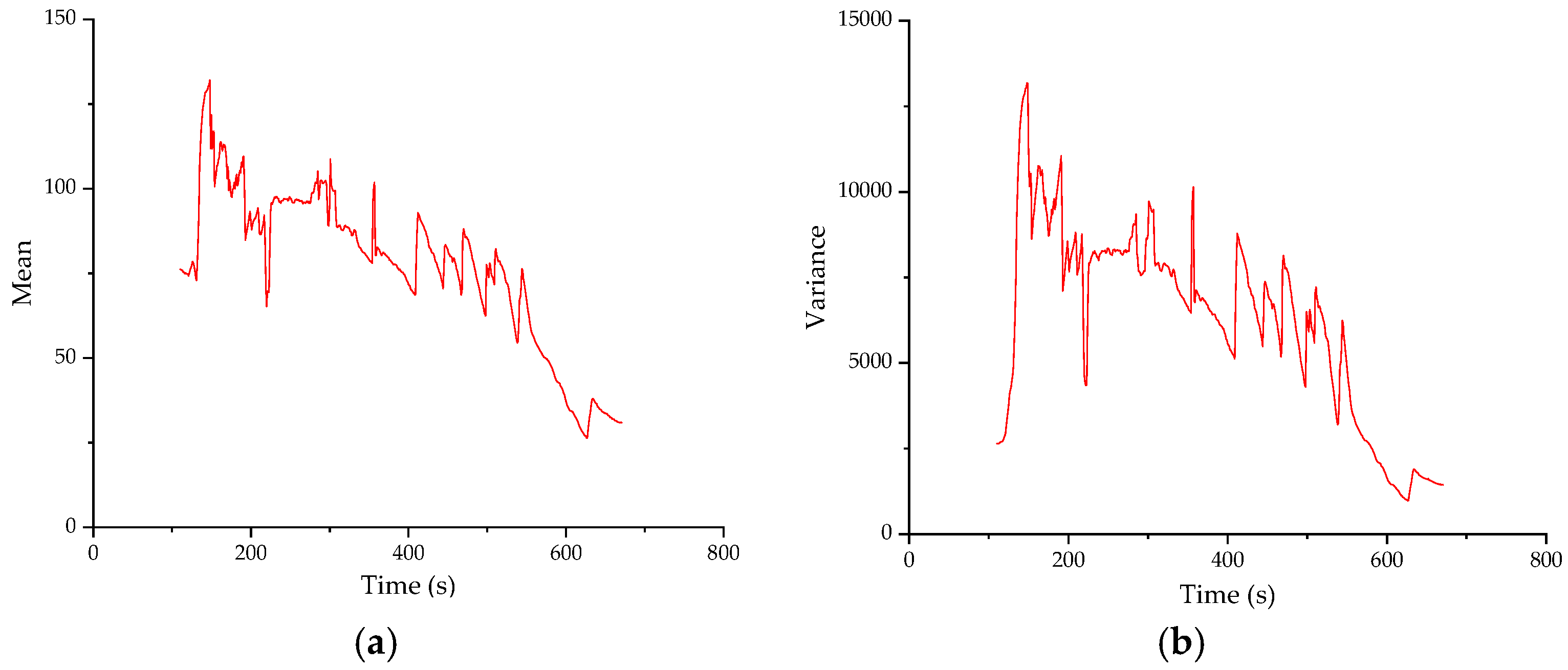
4.2.2. Extraction of Grey Features

(1)

Mean and variance of greyscale images

A similar method can be used to obtain the mean and variance of greyscale images. Firstly, the digital image information acquisition model is used to convert the original color image to grey scale. For each pixel of the grey scale, the mean value and variance of all pixels can be obtained through mathematical statistics.

$$\{\begin{array}{l}{\mu }_{grey}=\frac{1}{N}{\displaystyle \sum _i^{N}gre{y}_i}\\ {\sigma }_{grey}=\sqrt{\frac{1}{N}{\displaystyle \sum _{i=1}^N{(gre{y}_i-{\mu }_{grey})}^2}}\end{array}$$

(7)

where, μ_grey and σ_grey represent the variance and mean, respectively, of all the pixels in the grey image obtained by the transformation. grey_i represents the grey level of the i-th pixel in the grey image. N represents the total number of pixels in the greyscale image.

(2)

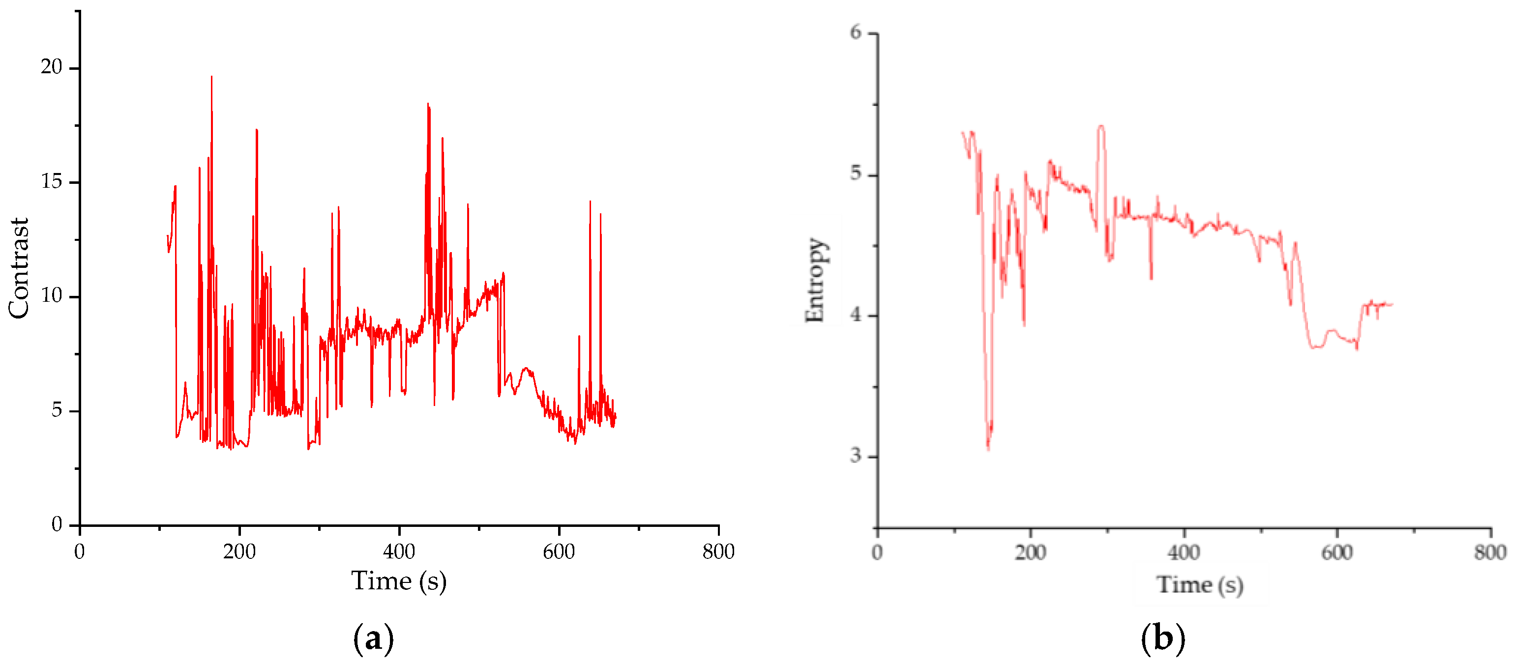
Entropy of greyscale images

Image entropy is expressed as the bit average of the image grey level, which describes the degree of non-uniformity or complexity of the texture in the image. For a two-dimensional image in discrete form, its information entropy can be calculated as follows:

$$\{\begin{array}{l}ent={\displaystyle \sum _{s=0}^{255}{P}_{st}{\log }_2{P}_{st}}\\ P_s=\frac{1}{N}f(s,t)\end{array}$$

(8)

where P_s is the number of times the grey value s appears in the image, and ent is the image entropy of the image. s represents the grey value of a pixel and t represents the mean value of the grey neighborhood of s. f(s,t) is the frequency of the feature binary group (s,t) appearing in the image. N is the total number of pixels in the greyscale image.

(3)

Contrast of greyscale images

Image contrast refers to the measurement of different levels of brightness between the brightest white and the darkest black in an image, namely, the size of the gray contrast of an image. The formula is as follows:

$$C_M=\frac{I_{\max }-I_{\min }}{I_{\max }+I_{\min }}$$

(9)

where C_M is the contrast of an image, I_max is the maximum brightness and I_min is the minimum brightness.

4.3. Principal Component Analysis of Image Information

Principal component analysis (PCA) [26] is a data dimensionality reduction method that can transform a large number of related data into a small number of unrelated data and reflect the information in the original data as much as possible.

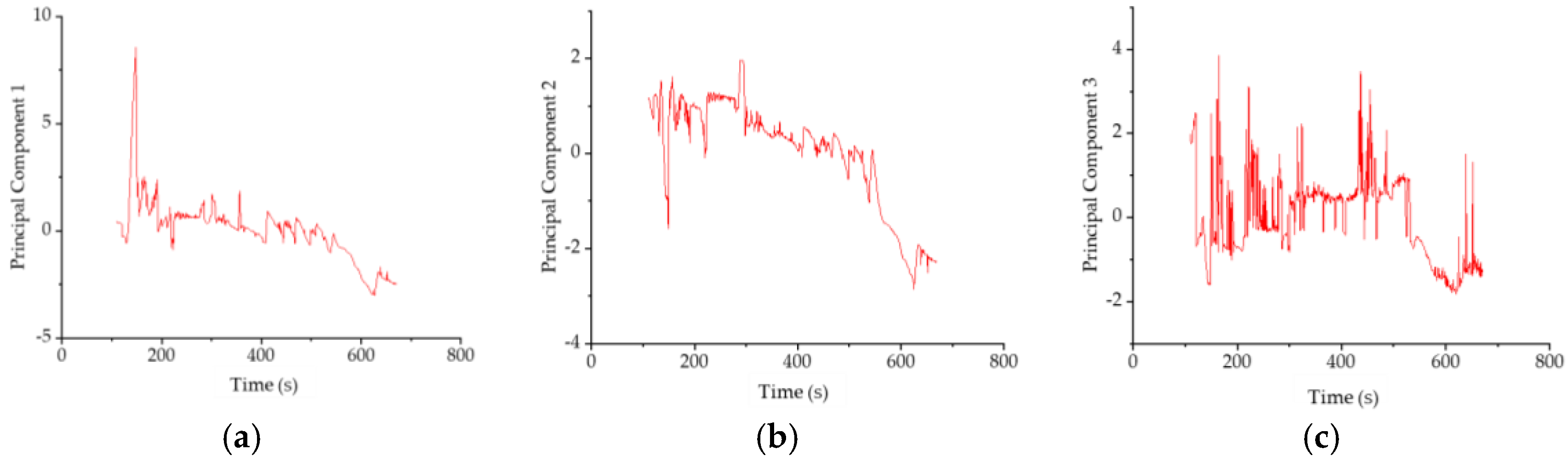
In the image feature extraction part, a total of ten features in the image were extracted. There is a certain correlation among the ten features, and different features have different dimensionalities. In order to fully exploit the information of the features and unify the dimensions, the PCA method is used to analyze the obtained image information and convert ten features into three main features. By constructing a comprehensive score model and using three main features, the comprehensive score of all the features can be obtained. Without PCA, it is difficult to make full use of the information of ten features.

Let s be the weighted sum of the information x₁, x₂,…, x_n extracted from the image (the weights are c₁, c₂,…, c_n).

$$s=c_1{x}_1+c_2{x}_2+\cdots +c_n{x}_n$$

(10)

Since the extracted information usually has different dimensions and orders of magnitude, it is necessary to first standardize the obtained data information. Assuming that the j-th data of the i-th information are x_ij, $\tilde{x}$_ij and $\tilde{x}$_j are the mean values, the processing method is as follows:

$$\{\begin{array}{l}{\tilde{x}}_{ij}=\frac{x_{ij}-{\tilde{x}}_j}{s_j}\\ {\tilde{x}}_j=\frac{1}{n}{\displaystyle \sum _{i=1}^n{x}_{ij}}\\ s_j=\frac{1}{n-1}{\displaystyle \sum _{i=1}^n{\left(x_{ij}-{\tilde{x}}_j\right)}^2}\end{array}$$

(11)

By choosing appropriate weights, the information in each photo can be better distinguished. Each photo corresponds to the sum of the weights, denoted s₁, s₂,…, s_j. If the distribution of the sum of the weights in these photos is scattered, it means that the group of weights can be well distinguished.

Let us assume that X₁, X₂,…, X_p are the random variables for the p-th information. Since the variance reflects how discrete the data are, it is possible to find a set of c₁, c₂,…, c_p that gives the maximum value in the following formula.

$$Var(c_1{X}_1+c_2{X}_2+L+c_p{X}_p)$$

(12)

This means that this group of weights can make the value of s the most scattered. In order for the weight obtained to be meaningful, it must also meet the following requirements:

$$c_1{}^2+c_2{}^2+\cdots +c_n{}^2=1$$

(13)

Under the constraint of Equation (13), the optimal solution of Equation (12) is a unit vector that represents a direction in the p-dimensional space, namely, the principal component direction. Since one principal component is not enough to represent all the original variables, more principal components need to be found. The second principal component should not contain any information from the first principal component, so the directions of all principal components should be orthogonal. Now assuming that Z_i is the i-th principal component, all principal components can be expressed as:

$$\{\begin{array}{l}{Z}_1=c_{11}{X}_1+c_{12}{X}_2+\cdots +c_{1p}{X}_p\\ Z_2=c_{21}{X}_1+c_{22}{X}_2+\cdots +c_{2p}{X}_p\\ \\ Z_p=c_{p1}{X}_1+c_{p2}{X}_2+\cdots +c_{pp}{X}_p\end{array}$$

(14)

For each Z, the maximum value of Formula (12) should be solved under the condition that Equation (13) is satisfied, and the vectors (c₁₁, c₁₂,…, c_1p), (c₂₁, c₂₂,…, c_2p),…, (c_p1, c_p2,…, c_pp) should not be perpendicular to each other.

During the solution process, the eigenvalue of each characteristic covariance matrix in the image, λ, can be obtained. This eigenvalue reflects the amount of original information retained by the principal component. The percentage variance of each principal component can be calculated from the eigenvalue, as follows:

$$p_i=\frac{{\lambda }_i}{{\displaystyle \sum _{t=1}^n{\lambda }_t}}\times 100\%$$

(15)

where p_i (p₁ < p₂ < … < p_i−1 < p_i < p_i+1 < … < p_n) refers to the variance percentage of the i-th principal component. The closer the variance percentage is to one, the more original information is retained in the principal component.

Since the main purpose of principal component analysis is to reduce the number of variables, a small number of principal components are usually selected in the principal component solution process to ensure that their cumulative contribution rate reaches 70% to 80%. The cumulative contribution rate q_i is defined as

$$q_i={\displaystyle \sum _{j=1}^i{p}_j}$$

(16)

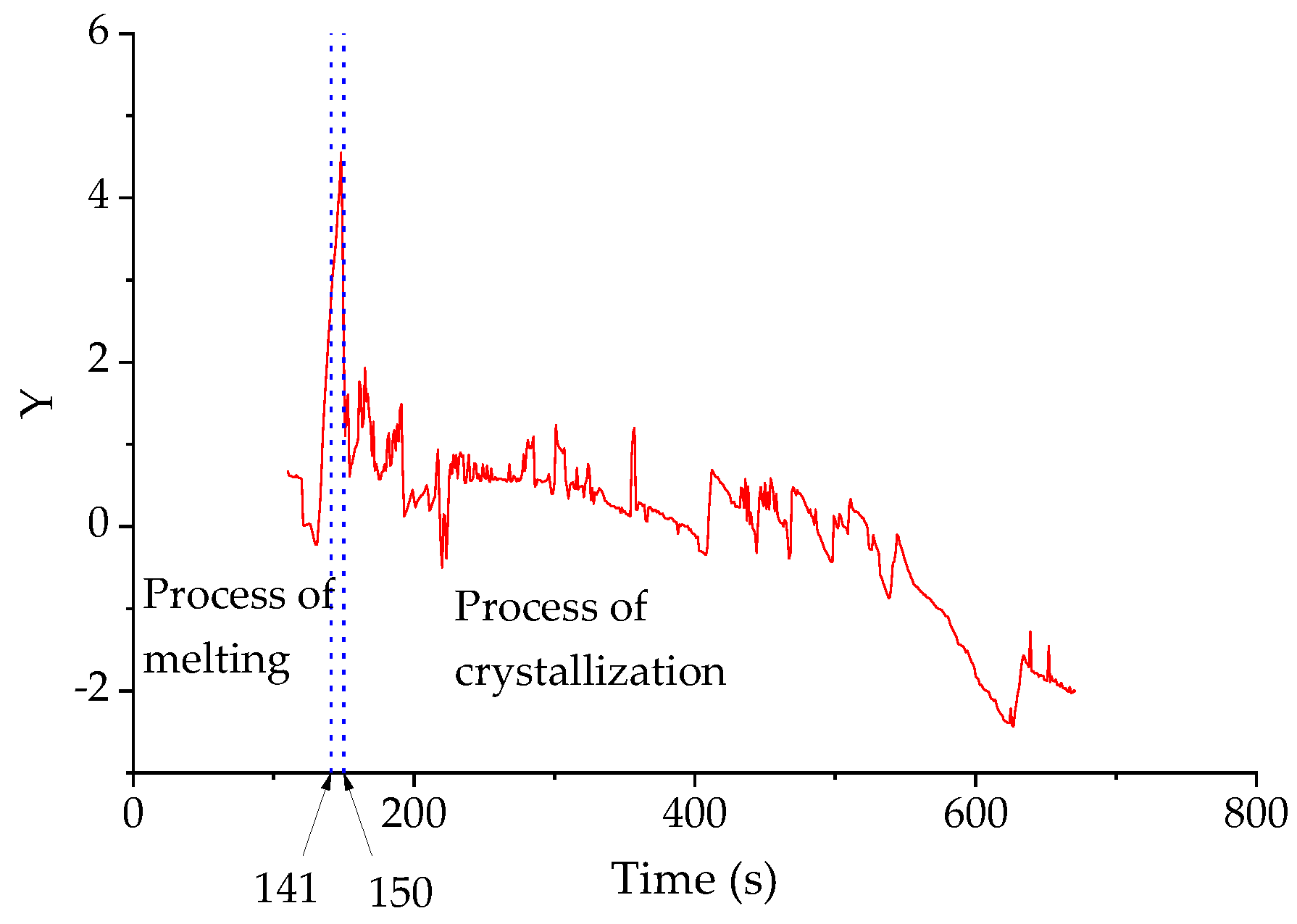
Suppose that k principal components have been selected by the cumulative contribution rate, and the function s(t) of k principal components over time has been calculated. The comprehensive score of the k principal components can be obtained from these variance percentages. The calculation method is as follows:

$$Y\left(t\right)={\displaystyle \sum _{i=1}^k{p}_i}{s}_i\left(t\right)$$

(17)

where, s_i(t) is the function of the i-th principal component changing with time at time t, and Y(t) is the comprehensive score of the k components over time.

4.4. Normalization of Comprehensive Score

Since the evaluation criteria of comprehensive scoring data are not the same, it is necessary to dimensionalize the value of Y and unify the evaluation criteria. Normalization is usually used to unify the dimensions. Through the linear change of the sample, the sample data are mapped to [0, 1], and the different dimensional expression of the sample is converted to the dimensionless expression. Its expression is as follows:

$$Y_{norm}^t=\frac{Y^t-Y_{\min }}{Y_{\max }-Y_{\min }}$$

(18)

where Y^t_norm is the t-th characteristic of vector norm.

4.5. Time Series Modeling of Image Information

The ARIMA model [27] is a well-developed time series prediction model, which is often used for prediction based on time series data. The image features of melting crystallization of mold flux are a data series with time, so the ARIMA model can be successfully used to analyze them. A typical ARIMA model, ARIMA(p, d, q), can be written as:

$$(1-{\displaystyle \sum _{i=1}^P{\varphi }_i{L}^i}){(1-L)}^d{X}_t=(1+{\displaystyle \sum _{i=1}^q{\theta }_i{L}^i}){\epsilon }_t$$

(19)

where L is a lag operator, satisfying d∈Z, d >A₀. ϕ_i is the autocorrelation coefficient, θ_i is the moving average coefficient and ε_t is the interference error. X_t represents the value of the time series at time t. As explained in Equation (19), in ARIMA(p, d, q), AR is “autoregressive”, and p is the order of autoregressive terms. MA is the “moving average”, q is the order of moving average terms and d is the number of differences made to make it a stationary sequence (order).

$$ARIMA(p,d,q)\{\begin{array}{l}AR(p)-\mathrm{autoregressive} \mathrm{coefficient} \mathrm{of} \mathrm{order} p\\ MA(q)-\mathrm{moving} \mathrm{average} \mathrm{coefficient} \mathrm{of} \mathrm{order} q\\ d-\mathrm{difference} \mathrm{order} \mathrm{needed} \mathrm{to} \mathrm{make} \mathrm{a} \mathrm{stationary} \mathrm{sequence}\end{array}$$

(20)

4.5.1. ADF Unit Root Test

Before establishing the ARIMA model, the data should be stabilized, that is, the data must be processed by the numerical difference method. The augmented Dickey–Fuller (ADF) unit root test can be used to determine the stationarity of a data set. For an AR(p) model, it can be rewritten as follows:

$$y_t={\displaystyle \sum _{i=1}^p{\varphi }_i{y}_{t-i}+{\epsilon }_t=}\rho y_{t-1}+{\displaystyle \sum _{i=1}^{p-1}{\zeta }_i\Delta y_{t-1}+{\epsilon }_t}$$

(21)

$$\rho ={\displaystyle \sum _{i=1}^p{\varphi }_i}$$

(22)

where y_t is the current image information sequence, t is the test statistic and ε_t is the serially independent error term at time t. ρ is the ordinary least squares (OLS) estimate (based on an p-observation time series) of the autocorrelation parameter.

4.5.2. Determination of ARIMA Model Parameters

Since the construction of AR (autoregressive) requires stationarity, the construction of ARIMA model also requires stationarity, the numerical difference method can be used to process the data. The first-order difference is the difference between t and t−1, the second-order difference is a difference based on the first-order difference, so that the number of differences after data stationarity is the parameter d that we want to determine. Therefore, continuous differential processing of the image information was performed to determine the final value of d.

In the ARIMA model, the order of the lag terms p and q should be determined by autocorrelation function (ACF) and partial autocorrelation function (PACF). The parameters p and q obtained are shown in

Table 1. Determination of the p and q order of the ARIMA model.

Models	ACF	PACF
AR(p)	degradation tends to 0 (geometric or oscillatory)	p-order posterior truncation
MA(q)	q-order posterior truncation	degradation tends to 0 (geometric or oscillatory)
ARMA (p, q)	q-order degradation tends to 0 (geometric or oscillatory)	p-order degradation tends to 0 (geometric or oscillatory)

.

Among them, when PACF is truncated after stage p, the truncation order is the parameter p determined by the model; when ACF is truncated after stage q, the truncation order is the parameter q determined by the model. The calculation method of ACF and PACF is described below.

ACF is a complete autocorrelation function that describes the degree of correlation between the current and past values of the sequence. ACF takes into account the trend and residual of the image information when searching for correlation, and its formula is as follows:

$$ACF(k)={\rho }_k=\frac{Cov(y_t,y_{t-k})}{Var(y_t)}$$

(23)

where y_t is the current sequence of image information, y_t−k is the k-order lag sequence of image information and ρ_k is the coefficient of the autocorrelation function between the current sequence and the k-order lag sequence of image information.

The partial autocorrelation function (PACF) only describes the relationship between the observed value and its lag term, that is, the relationship between the current image information sequence and the p-order lagged image information sequence, while adjusting for the influence of other shorter lag terms. The formula is:

$$R \Phi =r$$

(24)

By inverting it, we can obtain:

$${\Phi }^{\prime }={(R)}^{-1}r=\left(\begin{array}{c}{\Phi }_1\\ {\Phi }_2\\ ⋮\\ {\Phi }_p\end{array}\right)$$

(25)

where Φ′ is the autocorrelation coefficient of the lag period p, and Φ_p is the partial autocorrelation coefficient.

4.6. Relationship between Temperature, Melting Rate and Crystallizing Rate

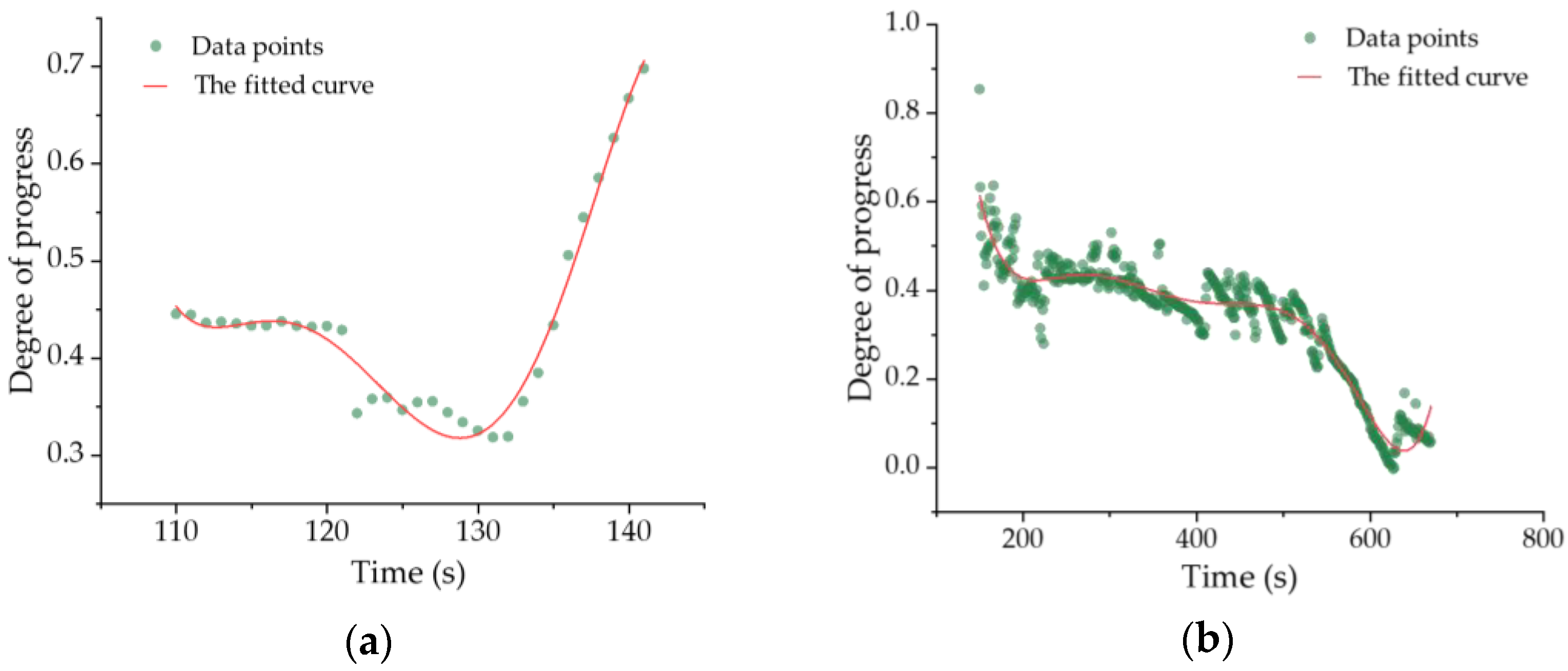
This part aims to obtain the relationship between temperature, time change and the melting and crystallization process of the mold flux based on the established time series model. Since temperature is linearly dependent on time, temperature can be expressed linearly by time. Therefore, the relationship between the melting and crystallization process of the mold flux and temperature can be converted into a relationship with time. For such problems, the least squares method, polynomial fitting and other methods can be used to fit them, so as to solve the melting and crystallization equation of the mold flux. In this paper, the bivariate polynomial fitting method under the least square method is used to obtain the functional relationship between the change of temperature, time and the melting and crystallization process of the slag. Assume that the function H(x) is a polynomial function, and its general formula is:

$$H\left(x\right)={\displaystyle \sum _{n=1}^N{a}_n{x}^{n-1}}$$

(26)

where a₁, a₂,…, a_n are the binomial coefficients, the best fitting value can be obtained by the least squares method, namely:

$$\begin{array}{l}\min G(a_1,a_2,\cdots a_n)={\displaystyle \sum _m{(H(x_m)-y_m)}^2}\\ s.t.\{\begin{array}{l}n,m>0\\ n,m\in N^{*}\end{array}\end{array}$$

(27)

where G(a₁, a₂, …, a_n) is the optimization objective of the least squares method, a₁, a₂,…, a_n are the binomial coefficients and x_m and y_m are the horizontal and vertical coordinates of the point m, respectively. When the binomial coefficient reaches a certain value, G(a₁, a₂,…, a_n) reaches the minimum value corresponding to the number of points where the binomial fitting effect is the best.

In the measurement process, the slag does not start melting or crystallizing at time 0. In order to better describe the melting and crystallization process. Time must be further converted.

$$\{\begin{array}{l}{t}_c=t-t_{c0}\\ t_m=t-t_{m0}\end{array}$$

(28)

where t_m0 and t_c0 represent the time of melting and crystallization, respectively. t_m and t_c represent the time of melting and crystallization after t time.

Since the relationship between the determined principal component and time can be obtained by polynomial fitting, it is assumed that the principal component and time satisfy a polynomial function:

$$H\left(t\right)={\displaystyle \sum _{n=1}^N{a}_n{t}^{n-1}}$$

(29)

The above function shows the relationship between time and the melting and crystallization process. Temperature is linearly correlated with time, which can be expressed as:

$$\{\begin{array}{l}{T}_c=k_c{t}_c-T_{c0}\\ T_m=k_m{t}_m-T_{m0}\end{array}$$

(30)

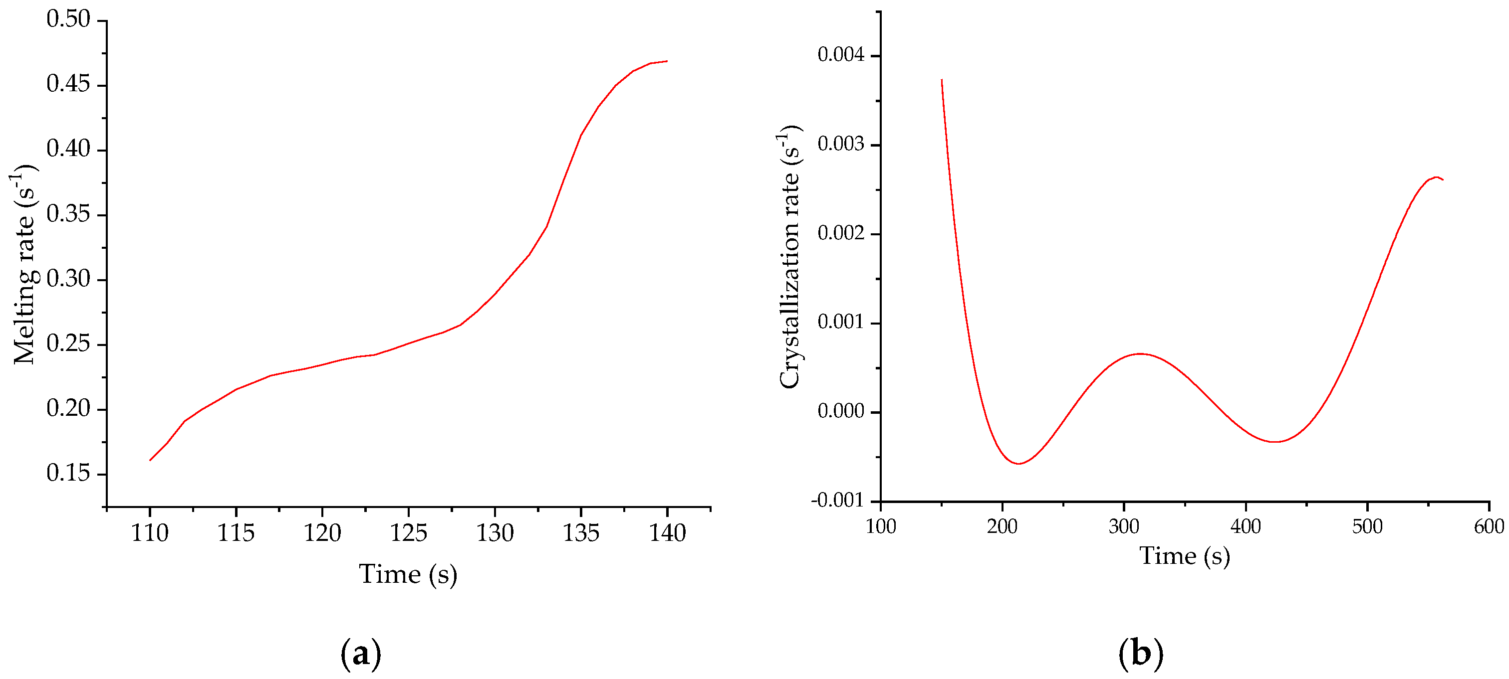
where T_m and T_c are the melting and crystallization temperatures after time t, respectively. T_m0 and T_c0 represent the temperatures at which melting and crystallization start, respectively. The relationship between time and temperature is linear, and the rate of melting and crystallization process can be expressed as:

$$\{\begin{array}{l}{v}_c\left(t_c\right)=-\frac{d}{dt}{H}_c(t_c)\\ v_m\left(t_m\right)=\frac{d}{dt}{H}_m(t_m)\end{array}$$

(31)

where v_m and v_c represent melting and crystallization rate, respectively. H_m(t_m) and H_c(t_c) represent the functional relationship between melting and crystallization process and time, respectively, that is, the relationship between the content of the selected principal component and the time. As the melting and crystallization rate are defined by the rate of change of the composite score, to avoid the crystallization rate value being less than 0, the crystallization rate was defined as the negative of the rate of change of the composite score. By combining Equation (30) with (31), we can obtain:

$$\{\begin{array}{l}{v}_c\left(\frac{T_c-T_c{}_0}{k_c}\right)=-\frac{d{H}_{{}_c}(\frac{T_c-T_c{}_0}{k})}{dt}=-\frac{1}{k_c}\frac{d{H}_c\left(T_c-T_c{}_0\right)}{dt}\\ v_m\left(\frac{T_m-T_m{}_0}{k_m}\right)=\frac{d{H}_m(\frac{T_m-T_m{}_0}{k})}{dt}=\frac{1}{k_m}\frac{d{H}_m\left(T_m-T_m{}_0\right)}{dt}\end{array}$$

(32)

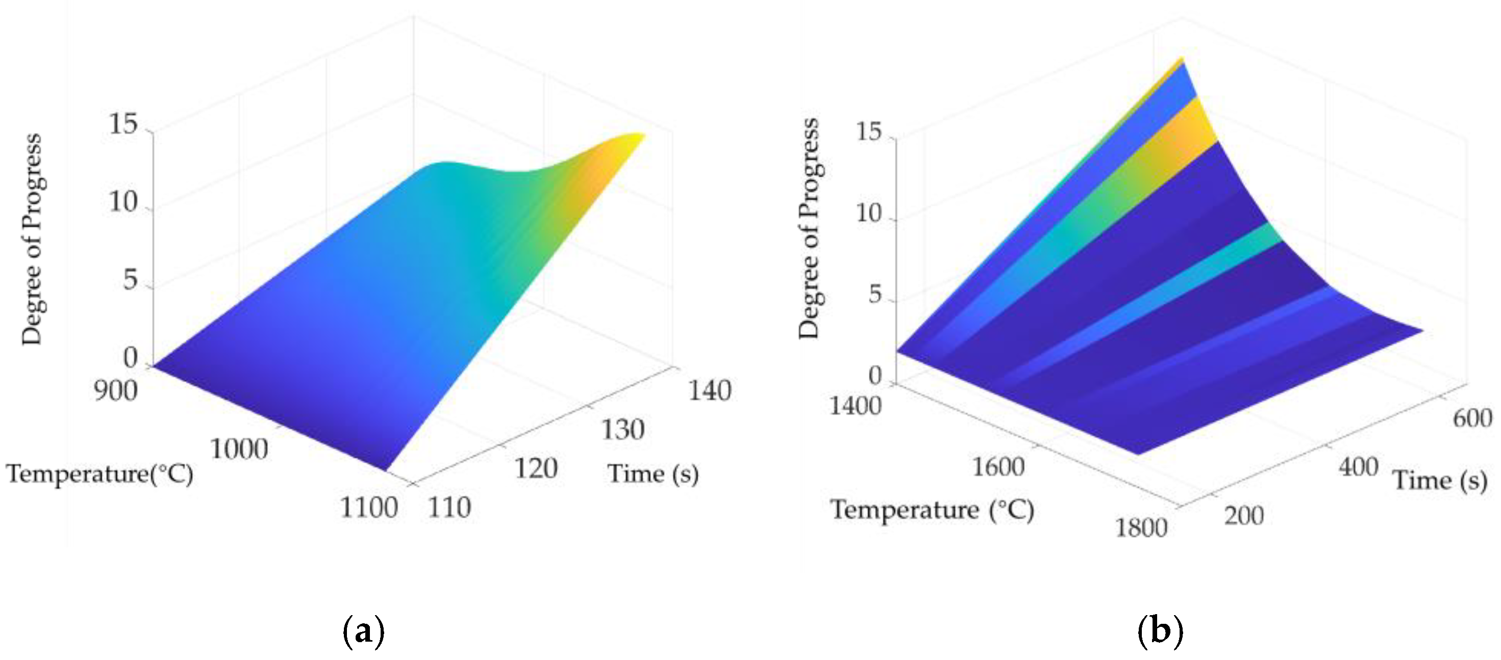
The function above shows the functional relationship between temperature and melting and crystallization rate. The process of melting and crystallization process can be further expressed as:

$$\{\begin{array}{l}{H}_c(t_c,T_c)=v_c(\frac{T_c-T_c{}_0}{k_c})t_c\\ H_m(t_m,T_m)=v_m(\frac{T_m-T_m{}_0}{k_m})t_m\end{array}$$

(33)

where H_m(t_m, T_m) and H_c(t_c, T_c) represent the melting and crystallization process after T_m, T_c time at t_m, t_c temperature, respectively, that is, the relationship between the content of the selected principle component and time and temperature.

5. Results

According to the algorithm process shown in Figure 5, the image after removing the background was first converted to grey level. Furthermore, by extracting the image feature information, the mean and variance of RGB, the mean and variance of grey and the contrast and entropy of the grey image during the melting and crystallization of the mold flux were obtained, respectively. Ten characteristic values were extracted, and three parameters of the ARIMA model were obtained by principal component analysis method, combined with ADF test and ACF tests. Finally, the melting and crystallization curves of the slag were analyzed based on the data of the components.

5.1. Results of Feature Extraction

Figure 6 shows the mean and variance of RGB in the melting and crystallization process. As can be seen in Figure 6, the mean value of the red component increases rapidly between 110 and 150 s and becomes stabilized between 150 and 580 s. The mean value of the green component fluctuates and decreases after a rapid increase. However, the mean value of the blue component changes very little throughout the melting and crystallization process. The change in the variance of the three colors is similar to the change in the mean.

Figure 7 shows the variation of the mean and variance of the greyscale over time. It can be seen that the mean and variance of the image greyscale are very close to each other over time. The mean and variance increased rapidly from 110 to about 150 s, and then showed a decrease in fluctuation.

Figure 8 shows the change in image contrast and entropy over time during the melting and crystallization process. The contrast ratio of the image fluctuates greatly over time. The contrast fluctuates significantly between 110 and 300 s and between 430 and 470 s. The entropy of the image also fluctuates significantly in the interval from 110 to 200 s, and the fluctuation of the entropy of the image slows down after 200 s. The overall entropy of the image shows a decreasing trend.

5.2. Determination of Principal Components

Since there are many features extracted from the image, in order to comprehensively consider various features, the 562 data sets of data of ten features extracted from the photo in the previous step were adopted by principal component analysis to obtain comprehensive features of the extracted features. The results of the analysis are shown in

Table 2. Parameters of the 10 principal components obtained from the principal component analysis.

Principal Component	Initial Eigenvalue			Extract the Sum of Loads Squared
	Total	Percentage of Variance (%)	Cumulative Percentage (%)	Total	Percentage of Variance (%)	Cumulative Percentage (%)
1	5.73	57.33	57.33	5.73	57.33	57.33
2	1.98	19.82	77.15	1.98	19.82	77.15
3	1.00	10.07	87.22	1.01	10.07	87.22
4	0.84	8.36	95.58	-	-	-
5	0.35	3.54	99.12	-	-	-
6	0.65	0.65	99.77	-	-	-
7	0.02	0.20	99.96	-	-	-
8	0.004	0.04	100.00	-	-	-
9	0.00	0.002	100.00	-	-	-
10	0.00	0.00	100.00	-	-	-

.

The table above lists the ten principal components obtained from the principal component analysis. Total refers to each eigenvalue of the correlation coefficient matrix of the extracted features. The variance percentage of the original eigenvalue reflects how much of the original information is retained by the component during the principal component analysis. Based on the cumulative contribution rate of each principal component, principal components 1, 2 and 3 were selected as the final principal components.

Table 3. Principal component loads of principal components 1, 2, and 3.

Extract Features	Principal Components
	1	2	3
Grey mean	0.4	0.18	0.01
Grey variance	0.4	0.16	−0.09
R mean	0.39	−0.13	−0.01
G variance	0.38	0.24	−0.1
G mean	0.37	0.28	0.01
R variance	0.36	−0.23	−0.06
Entropy	0.23	−0.17	0.34
B variance	−0.06	0.66	−0.01
B mean	−0.23	0.51	0.29
Contrast	0.1	−0.08	0.88

shows the component matrix of principal components 1, 2 and 3, from which the load of each feature on different principal components can be obtained.

As can be seen from the table, the grey mean, grey variance, R mean, G variance, G mean and R variance have a large load on principal component 1, indicating that they have a high correlation coefficient with principal component 1. The variance of B has greater load on principal component 2, indicating that it has a higher correlation coefficient with principal component 2. The contrast of the load on principal component 3 is greater, indicating that it has a higher correlation coefficient with principal component 3. Based on the loadings of principal components 1, 2 and 3 listed in Table 3, and the standardized results of the value of each feature at each moment, the contents of the principal component at each moment can be calculated. The contents of principal components 1, 2 and 3 change over time as shown in Figure 9.

Using the changes of the three principal components over time and their variance percentage, the change curve of the comprehensive score Y of the three principal components over time can be obtained, as shown in Figure 10.

From 110 to 150 s, the comprehensive score shows an upward trend, and from 150 to 671 s, comprehensive score Y shows a fluctuating downward trend over time. The variation trend of comprehensive score Y over time is basically consistent with the melting and crystallization process of mold flux. To a certain extent, the comprehensive score Y can reflect the melting and crystallization process of mold flux well.

For the comprehensive score, the weights of principal components 1, 2 and 3 are 65.7%, 22.7% and 11.6%, respectively. Therefore, principal component 1 has the greatest influence on the overall score. The loadings of grey mean, grey variance, R mean, G variance, G mean and R variance are relatively large. The melting process time is short and the changes of characteristics are obvious, which means that the melting speed of the mold flux is high and the color and texture changes are obvious. However, the crystallization rate is relatively small, the color and texture of the mold flux in the early crystallization period are not obvious and the change of color and texture in the late crystallization period is obvious.

5.3. Results of the Time Series Model

Then, the ADF test was used to analyze the stationarity of the two principal component’s data. According to the p value, it is found that the data can meet the requirements of stationarity analysis and finally

Table 4. ADF inspection results.

Difference Order d	t	p	Critical Value
			1%	5%	10%
0	−0.803	0.818	−3.442	−2.867	−2.570
1	−8.840	0.000	−3.442	−2.867	−2.570

was obtained.

As shown in Table 4, the p-value of the data is less than 0.05 when the difference order of difference is 1. Partial (self) correlation detection was then performed on the data, and ACF and PACF plots were obtained. The regression order and the moving average order of the data can be obtained by combining them, as shown in

Table 5. Autoregressive order and moving average order of the ARIMA model.

Category	Autoregressive Order p	Moving Average Order q
Orders	4	4

.

So far, the difference order, the regression order and the moving average order of the principal component have been obtained. The three orders correspond to the three parameters of the ARIMA model, that is, ARIMA time series modeling can be carried out. The principal component corresponds to the ARIMA(4,1,4) model. The melting and crystallization curves of the slag were discussed with the data of the principal component.

In this model, ten features of the image were extracted, and the dimensions of the ten features were reduced to one principal component by principal component analysis and weighted average, and the parameters of the ARIMA model of the principal component were determined by ACF and ADF tests, thus the melting and crystallization curves were analyzed.

5.4. Relationship between Crystallization-Temperature and Time

The relationships between temperature and time during the melting and crystallization process were calculated and are shown in

Table 6. Relationships between temperature and time.

Process	k	T0	R2	RMSE
Melting	5.98	887.01	0.9632	10.76
Crystallization	−1.97	1840.50	0.9996	3.829

.

Table 6 shows all the parameters of the linear relationship between temperature and time, where R² is the degree of fit between temperature and time. The closer R² is to 1, the better the fit. RMSE [28] is the root mean square error. In the process of melting and crystallization, the relationship between temperature and time is satisfied:

$$\begin{array}{l}Melting:T=5.98t+T_0\\ Crysatllization:T=-1.97t+T_0\end{array}$$

(34)

Principal component 1 obtained above was put into the mathematical model as a physical quantity to measure the progress, and the relationship between melting and crystallization progress and time was obtained by MATLAB, respectively. The final fitting result of time and melting and crystallization progress depends on the choice of polynomial term n. If n is too small, an underfitting phenomenon may occur, which cannot truly reflect the relationship. If n is too large, overfitting may occur. For melting and crystallization, n = 5 and 6 were used for fitting, respectively. The fitting results of the melting process are shown in Figure 11.

Figure 11 shows the polynomial fitting results of melting progress, crystallization progress and time, respectively. The x-coordinate is time, and the y-coordinate is melting or crystallization progress. The red solid lines are the fitted curves for the melting and crystallization when the polynomial degree is 5 and 6, respectively, and the green round dot represents the fitted data point. The goodness of fit of the melting and crystallization process were 0.9714 and 0.9150, respectively. The RMSEs are 0.01834 and 0.04037, respectively. The fitting function is as follows:

$$\{\begin{array}{ll}{H}_c\left(t\right)=& -4.28\times {10}^{-7}{t_c}^5+2.69\times {10}^{-4}{t_c}^4-6.67\times {10}^{-5}{t_c}^3-8.36{t_c}^2-520.00t_c+1.29\times {10}^4\\ H_m\left(t\right)=& 5.15\times {10}^{-15}{t_c}^6-1.16\times {10}^{-11}{t_c}^5+1.05\times {10}^{-8}{t_c}^4-4.88\times {10}^{-6}{t_c}^3\\ & +1.22\times {10}^{-3}{t_c}^2-0.15t_c+8.19\end{array}$$

(35)

Now, the obtained fitting results of melting time and melting progress, as well as the fitting results of crystallization time and crystallization progress, were inserted into Equation (31) to obtain the curves of melting rate and crystallization rate. The results are shown in Figure 12.

Figure 12 shows the relationship between melting and crystallization rates as a function of temperature. (a) and (b) show the relationship between melting and crystallization rates and time, which are also referred to as melting kinetics and crystallization kinetics of the mold flux.

As can be seen from Figure 12a, it is easy to understand, but for Figure 12b, when the time is around 210 s and 425 s, the crystallization rate has an abnormal phenomenon of less than 0. This is due to the abnormal growth of the fitted rate curve during these two periods (as shown in Figure 11b). This is because in the process of material crystallization, in some periods, the change of the image is not obvious, and even reverse changes occur. In addition, there are some errors generated in the fitting process. The combination of the two reasons finally leads to such a result, which is in accord with the actual situation.

The functional relationship between temperature and time has been determined. According to the relationship obtained above as well as Equation (33), a functional relationship between the temperature, time and the melting and crystallization process of the mold flux was established. The areas represented by the bivariate functions of the two processes are shown in Figure 13.

Figure 13a,b shows the relationship between the crystallization volume ratio (degree of progress), temperature and time during the melting and crystallization processes of mold flux. Each point on the curve represents the volume ratio of crystallization at the current temperature T and the process time t. In the above figure, the larger the z-axis value of the surface, the more crystals there are in the current state.

In Figure 13, there is a phenomenon that the crystallization volume ratio exceeds the theoretically possible volume ratio. The reasons may be as follows:

First of all, when solving the kinetic model, the melting and crystallization were discussed separately. The time between the two stages is not continuous, which is different from the actual situation, which may lead to the differences between the actual melting (or crystallization) time and the current time used in the model.

Secondly, the polynomial fitting method may lead to the deviation between the melting rate at a certain temperature and the actual melting rate in the solving process.

Finally, the amount of data used for fitting in Figure 11a is small, which may lead to deviations between the melting rate at different temperatures and the actual value in the subsequent solving process.

6. Discussion and Conclusions

6.1. Discussion

In this paper, the image information was comprehensively considered, the main features of the image were determined and the dimension was reduced by principal component analysis. The accuracy and robustness of the model can be improved by exploiting the information provided by the image as much as possible, so that the accuracy of the model can be guaranteed even when some information is disturbed.

The binomial curve fitting was used to fit the melting and crystallization degree curve of the mold flux with time. As the fitted curve could not completely replace the original curve, it could introduce errors into the final results. In the previous section, the abnormal phenomenon of less than 0 in the crystallization rate curve was caused by this error. The errors generated in the fitting process will be analyzed quantitatively.

The deviation between the fitted result and the original data can be seen from the RMSE value obtained in the fitting process. Since this value is related not only to the deviation but also to the size of the original data, the relative root mean square error (RRMSE) [29] is now used to measure the error generated by the fitting, which is defined as the ratio of the RMSE to the mean of the original data, namely:

$$RRMSE=\frac{n}{{\displaystyle \sum _{i=1}^n{m}_i}}\cdot RMSE$$

(36)

and:

$$RMSE=\sqrt{\frac{1}{n}{\displaystyle \sum _{i=1}^n{\left(m_i-f\left(i\right)\right)}^2}}$$

(37)

where RRMSE is the ratio of the RMSE to the mean value of the original data and m_i is the i-th original data. In Equation (37), m_i is the original data before fitting and f(i) is the function value after fitting. N is the total number of raw data.

The RRMSE value of each fitting procedure can be obtained through the above equation. The RMSE and RRMSE values of all fitting processes are shown in

Table 7. RMSE and RRMSE values for all fitting methods used in this paper.

Dependent Variable of Fitting	Independent Variable of Fitting	RMSE	RRMSE
Melting temperature	time	10.76000	0.0110
Crystallization temperature	time	3.82900	0.0033
Comprehensive score of Melting	time	0.01834	0.0425
Comprehensive score of Crystallization	time	0.04037	0.1206

. The RRMSE can reflect the relative deviation between the fitting results and the original data. This value is independent of the original data, which can be used to better evaluate the fitting results.

It can be seen from Table 7 that the RRMSE of crystallization is larger than that of other fitting processes, indicating that the deviation is larger. This may be due to the more complex variation of the comprehensive score in the crystallization fitting process and the larger deviation of the polynomial fitting. In the following sections, the deviation generated in the melting and crystallization process will be calculated by using the following accumulative error ARRMSE.

$$ARRMSE=\sqrt{RRMS{E}_1{}^2+RRMS{E}_2{}^2}$$

(38)

In Equation (38), ARRMSE represents the cumulative relative root mean square error. RRMSE₁ and RRMSE₂ represent the errors of two fitting methods used for melting or crystallization, respectively. The deviation after two fits can be reflected by Equation (38). The larger the value, the greater the deviation after two fits.

For the problem discussed in this study. The ARRMSE of the melting process is 0.0439 and that of the crystallization process is 0.1207. The ARRMSE in the crystallization process is obviously greater than that in the melting process. The main reason is that the fitting error of the crystallization comprehensive score is relatively large. By comparing the RRMSE and ARRMSE fitted each time, it can be seen that the RRMSE with comprehensive score is close to the final ARRMSE in the two processes of melting and crystallization. It indicates that the fitting of the comprehensive score produces a much larger deviation than the fitting of the temperature. This may be because the relationship between comprehensive score and time is more complex, and the effect of polynomial fitting is not ideal. In addition, it can also be seen that reducing the deviation of the comprehensive score fitting is more important to improve the progress of the model. The deviation in this process can be reduced by switching to other fitting methods or increasing the amount of data.

Besides, some of the calculations may contain further errors: Firstly, in the extraction of temperature–time information, the image recognition ability depends on the established matrix of standard digital binarization information, only the digital information recognition function is realized in the image. Secondly, the image is processed by removing the background. This process will be affected by the boundary conditions of the background, and the number of pixels obtained after removing the background may be different, which may lead to certain errors in the process of image information extraction. Lastly, in the process of using the principal component analysis method to process image information, the principal component analysis method cannot make full use of all the image information and will ignore part of the information extracted from the image, which may lead to errors in the analysis process. At present, it is still difficult to calculate the above error quantitatively, and this is a very worthwhile study for the future.

6.2. Conclusions

By identifying the digital information in the upper left corner of the image and comparing it with the standard digital information, the time information of each image was obtained, and then the curve of the melting temperature of the mold flux changing with time was drawn. The digital recognition accuracy of this method is relatively high, which can meet the actual demand. Based on the image recognition technology, the automatic recognition of the temperature and time in the process of melting crystallization process of mold flux was successfully realized.

Based on the collected images, the dynamic difference between adjacent sequence images during melting and crystallization was investigated by using digital image processing technology. For the image information, ten features were extracted after removing the background, principal component analysis was used to reduce the dimension of the features, and three principal components were obtained and compared. The comprehensive score Y was calculated, normalized and used to reflect the melting and crystallization process of the mold flux.

Considering the influence of the change of temperature and time on the melting and crystallization progress of the mold flux, the relationship between time and temperature was fitted, and then a mathematical model was established to study the melting and crystallization kinetics of the mold flux (the relationship between temperature, melting rate and crystallization rate). The mathematical model established in this paper has high generality and can be successfully used for feature extraction and modeling analysis of molten crystal sequence images of mold flux.

Nevertheless, there are still some shortcomings in this study: (1) In the discussion section, possible sources of error are explained. Although the errors in the work in this paper are controllable, they still exist. In the future, relevant models can be improved to improve their calculation accuracy. (2) Time series model, principal component analysis and other methods are relatively traditional. Some new methods can be tried, compared and used to further improve the accuracy of the model. (3) The correlation fitting method can still be improved. (4) The study presented here used images from only one cycle and did not compare with images from multiple sets of parallel experiments. Although one set of experimental images may support the conclusion of this paper, the study of multiple parallel control groups is also a direction worth exploring in the future.