On the Definition of Phase Diagram

Abstract

A phase diagram, which is understood as a graphical representation of the physical states of materials under varied temperature and pressure conditions, is one of the basic concepts employed in high-pressure research. Its general definition refers to the equilibrium state and stability limits of particular phases, which set the stage for its terms of use. In the literature, however, a phase diagram often appears as an umbrella category for any pressure–temperature chart that presents not only equilibrium phases, but also metastable states. The current situation is confusing and may lead to severe misunderstandings. This opinion paper reviews the use of the “phase diagram” term in many aspects of scientific research and suggests some further clarifications. Moreover, this article can serve as a starting point for a discussion on the refined definition of the phase diagram, which is required in view of the paradigm shift driven by recent results obtained using emerging experimental techniques.

1. Introduction

In their pioneering work on semantics, semiotics, and the science of symbolism, published almost a century ago, Ogden and Richards recounted: “In all discussions we shall find that what is said is only in part determined by the things to which the speaker is referring. Often without a clear consciousness of the fact, people have preoccupations which determine their use of words. Unless we are aware of their purposes and interests at the moment, we shall not know what they are talking about and whether their referents are the same as ours or not” [1]. Today, this statement is still very true, even in the scientific language, where precise definitions are to be generally agreed upon. One of the frequently used and, at the same time, elusive physico-chemical terms that defies a single accepted definition is phase diagram. This expression is not reported in the IUPAC Gold Book [2], nor in the IUCr Online Dictionary of Crystallography [3]. In a recent review on pressure-induced phase transitions, Grochala noted that “the phase diagram is in its most common meaning a graph in which a property or a state of matter is shown in the function of pressure and temperature,” adding a caveat about the described system being in equilibrium [4]. Therefore, I decided to use the following general Oxford English Dictionary (OED) definition [5] as a reference point:

• phase diagram n. Chemistry a diagram which represents the limits of stability of the various phases of a chemical system at equilibrium, with respect to two or more variables (commonly composition and temperature); an equilibrium diagram.

In the high-pressure research, phase diagrams are usually constructed for systems of constant composition (empirical formula), with two variables: temperature (T) and pressure (P). Hence, the OED definition applied to the P–T space assumes that: (1) the limits of the stability of the phases are represented in a P–T chart as separate fields that correspond to each phase and are delimited by phase-boundary lines, also known as coexistence curves (representing the P–T conditions at which phase transitions occur), or the abscissa and ordinate axes (representing the P = 0 isobar and T = 0 isotherm, respectively); (2) phase diagrams pertain only to the equilibrium state. Note that the stability conditions may be ambiguous, as there are various definitions of stability (this will be discussed in more detail later). The OED definition therefore describes an ideal phase diagram, and it will be referred to as such from here onwards.

The phase diagrams published in the literature are determined in experimental studies or are predicted using various theoretical approaches. Both methods have their intrinsic limitations. In predicted phase diagrams, the boundary lines between the crystalline phases and melting curves are usually constructed by comparing the Gibbs free energies of individual phases. Because they can be computed using different models and approximations that also include temperature effects, the plots reported by various authors may differ significantly. On the contrary, the disagreements between experimental phase diagrams depend not only on the laboratory protocols, but also on the character of the phase transition.

To aid the reader and for clarity, a glossary of key terms related to the concept of the phase diagram is provided below.

2. Glossary of the Key Terms Related to Phase Diagrams

• An ideal phase diagram is a P–T plot of thermodynamically stable phases in the equilibrium state. There is only one ideal phase diagram for any stoichiometric assembly of atomic species. It is impossible to experimentally determine an ideal phase diagram because all experiments are dynamic, hysteresis in first-order phase transitions cannot be completely eliminated, and nonhydrostatic stresses and P,T gradients are inevitable;
• A phase diagram is the best estimate of the ideal phase diagram based on experimental and theoretical constraints;
• A dynamic P–T diagram represents observed or predicted phases that can be produced during the course of dynamic compression or decompression (or cooling/heating). A dynamic P–T diagram can include metastable or transitional states and must include descriptions of the necessary conditions: the compression or decompression rate, cooling or heating rate, stress–strain conditions, etc. Note that some authors refer to dynamic P–T diagrams as “dynamic phase diagrams”. The reason for this discrepancy is related to the definition of a phase, and the question of whether the thermodynamic metastable state can be regarded a phase. While a full discussion of this issue is beyond this opinion paper’s scope, I am leaning towards using the first option (i.e., a dynamic P–T diagram);
• A transitional P–T diagram (sometimes referred to as a transitional phase diagram) represents the P–T diagram that includes metastable states (i.e., the states outside of the stability region in the ideal phase diagram). Contrary to an ideal phase diagram, a transitional P–T diagram depicts a system that is far from thermodynamic equilibrium;
• The difference between dynamic and transitional diagrams can be characterized as semantic rather than phenomenological. The term dynamic P–T diagram is used mainly in dynamic-loading studies, where fast pressure variation is the intrinsic feature of the experimental methodology (shock compression, ramp compression, piezo-electrically driven dynamic diamond-anvil cells), and the observed states often have very short lifetimes. A transitional P–T diagram applies mostly to quasistatic experiments, where metastable states are “quenched” from the initial thermodynamic equilibrium and can be stabilized for a relatively long time (from minutes to years). This type of P–T diagram is largely related to multicomponent materials, but it can also describe chemical elements. For example, a transitional P–T diagram of buckminsterfullerene (C₆₀) reports the forms of carbon in which the molecular integrity of a C₆₀ molecule is preserved. It is different than the ideal phase diagram of carbon, as all the states of carbon consisting of C₆₀ molecules are metastable under any P–T condition. Note that there are also other terms used to convey similar notions, such as phase evolution diagram or kinetic phase diagram [6]. The term metastable phase diagram, which sometimes occurs in the literature, is ambiguous and should be abandoned;
• By using terms such as reaction P–T diagram [7] or transformation P–T diagram [8], some authors intend to emphasize that the transitions between different phases or states displayed on a diagram involve chemical reactions and the rearrangement of the bonding pattern (e.g., transformations from a molecular to an extended solid), although this additional specification seems redundant given the previously defined types of P–T diagrams.

3. Classification of Phase Transitions and Definitions of Phase Stability

In the most basic terms, phase transitions are usually related to the transformations of the physical properties of matter, which can be quantified by a change in the state parameters. The concept of a phase-transition order was introduced by Paul Ehrenfest in 1933 [9,10,11]. Ehrenfest’s approach is purely thermodynamic: Assuming that the thermodynamic potential (usually the Gibbs free energy (G) or chemical potential (μ)) is continuous across the phase boundary of any equilibrium phase transition, one can investigate its particular derivatives concerning an external thermodynamic variable, such as temperature or pressure. Hence, in the general case, for an nth-order phase transition:

$$\Delta {\left(\frac{{\partial }^{n}G}{\partial T^n}\right)}_P\ne 0; \Delta {\left(\frac{{\partial }^{n-1}G}{\partial T^{n-1}}\right)}_P=0 \mathrm{at}T=T_{trans},$$

(1)

$$\Delta {\left(\frac{{\partial }^{n}G}{\partial P^n}\right)}_T\ne 0; \Delta {\left(\frac{{\partial }^{n-1}G}{\partial P^{n-1}}\right)}_T=0 at P=P_{trans},$$

(2)

where G represents the Gibbs free energy, and T_trans and P_trans are the equilibrium transition temperature and pressure, respectively. Thus, the order of the transition is determined by the lowest nonzero derivative of the thermodynamic potential. At a first-order transition, the first derivatives of the G (namely, entropy (S) and volume (V)) are discontinuous; at a second-order transition, the S and V are continuous, but the second derivatives of the G (for instance, the constant-pressure heat capacity (C_P), the isothermal compressibility (β_T), and the isobaric thermal expansion coefficient (α)) are discontinuous, and so on. This simple view, however, is often inadequate for the characterization of some more complex transitions beyond the first order, which cannot be effectively described by a jump in any nth derivative of the thermodynamic potential, but by the nonanalytic behavior of these functions. In the modern classification scheme, which is essentially a generalization of the Ehrenfest one, phase transitions are classified into two broad categories: (1) “discontinuous” first-order transitions, which are distinguished by the presence of the latent heat and discontinuity in the order parameter defined on the grounds of the phenomenological theory formulated by Lev Landau [12]; (2) “continuous” second-order transitions (also comprising higher-order transitions, as defined in the Ehrenfest scheme), which are marked by a steady evolution of the order parameters, which are fully reversible across the phase boundary. This claim has significant consequences for the experimental determination of phase diagrams.

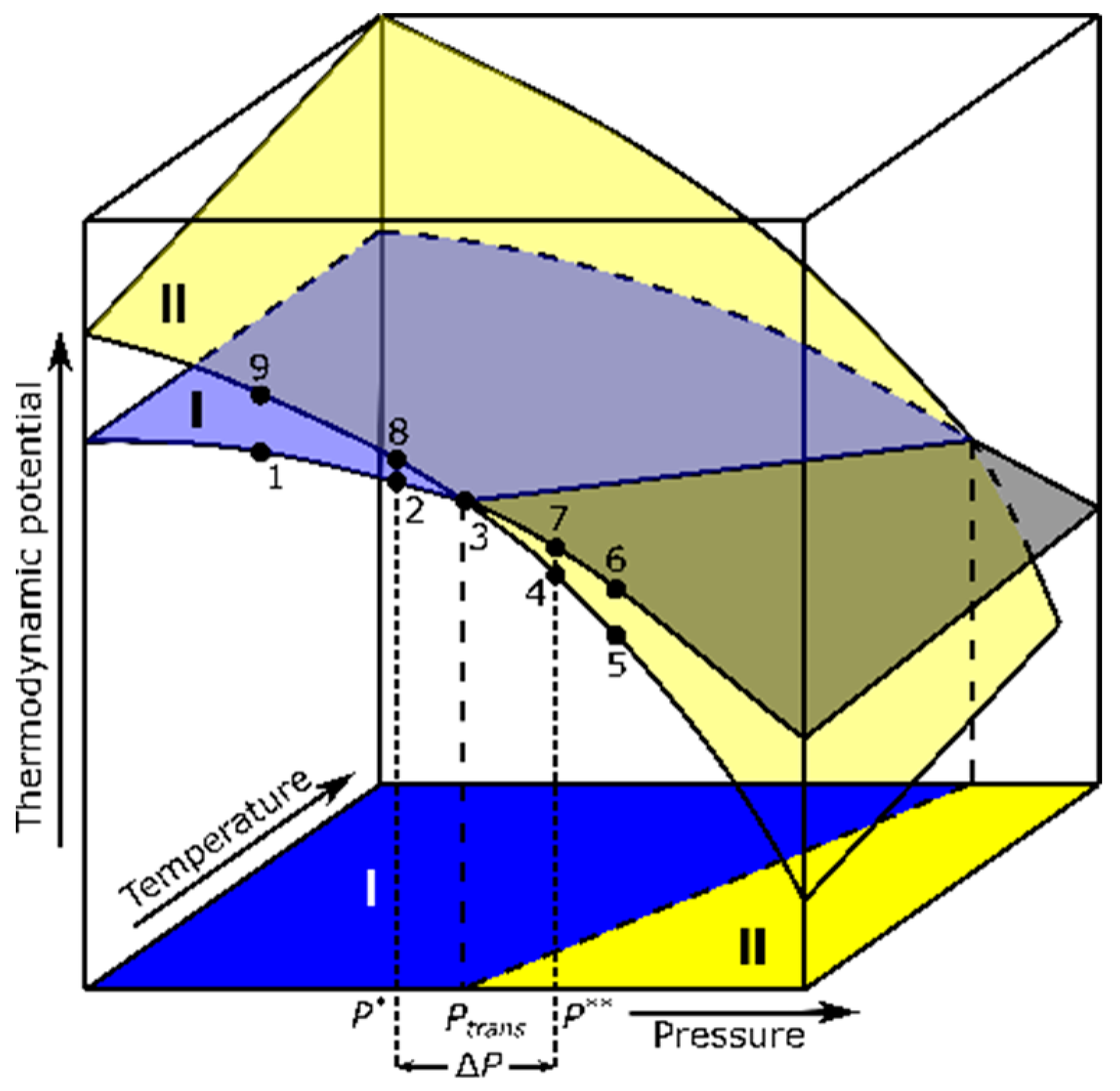
Consider a multidimensional space where the thermodynamic potential is a function of different variables. In a system of constant composition, each phase can be represented as a potential-energy surface in terms of pressure and temperature. The equilibrium-transformation conditions between two phases are defined by the intersection of surfaces, corresponding to the phase-boundary lines. In the example shown in Figure 1, if an isothermal compression is considered, then one can expect that the thermodynamic potential of the system should vary along the path 1–2–3–4–5 upon compression (5–4–3–2–1 upon decompression), with the sharp transformation of the entire sample occurring at Point 3, corresponding to the pressure (P_trans) at which the potentials of Phases I and II become equal. In practice, however, during the course of first-order transitions, the potential often follows the path 1–2–3–7–4–5 upon compression (5–4–3–8–2–1 upon decompression). Phase I, which exists for P_trans < P < P** during compression, is not in equilibrium because it is not the minimum potential configuration but a “superpressurized” metastable state. Likewise, Phase II, which persists upon decompression for P* < P < P_trans, corresponds to a “superdepressurized” state (named by an analogy to superheated and supercooled states). Hence, the experimental onset of the transition upon the pressure increase can be regarded as an upper bound of the metastability range, while the onset of the reverse transition marks a lower bound. The pressure range ΔP = P** − P* of this hysteresis (and the values of P* and P**) depend on many factors, such as the pressure-change rate and the purity of the substance. Moreover, note that the intervals (P**, P_trans) and (P_trans, P*) are not necessarily equal, and so the center of the hysteresis loop does not need to coincide with the transition pressure. Therefore, the actual value of the P_trans is difficult, if not virtually impossible, to locate from the experiment.

One of the most common examples is the first-order solid–liquid phase transitions and the determination of the melting line. In the isothermal runs, crystallization often occurs from the superpressurized liquid, while in standard experimental settings, virtually all the solids melt immediately under the equilibrium solid–liquid coexistence conditions without entering the underpressurized (superdepressurized) state. The reason behind this is that, in the case of heterogeneous melting, the crystal surfaces and grain boundaries suppress the energy barrier required for melt nucleation [13,14,15].

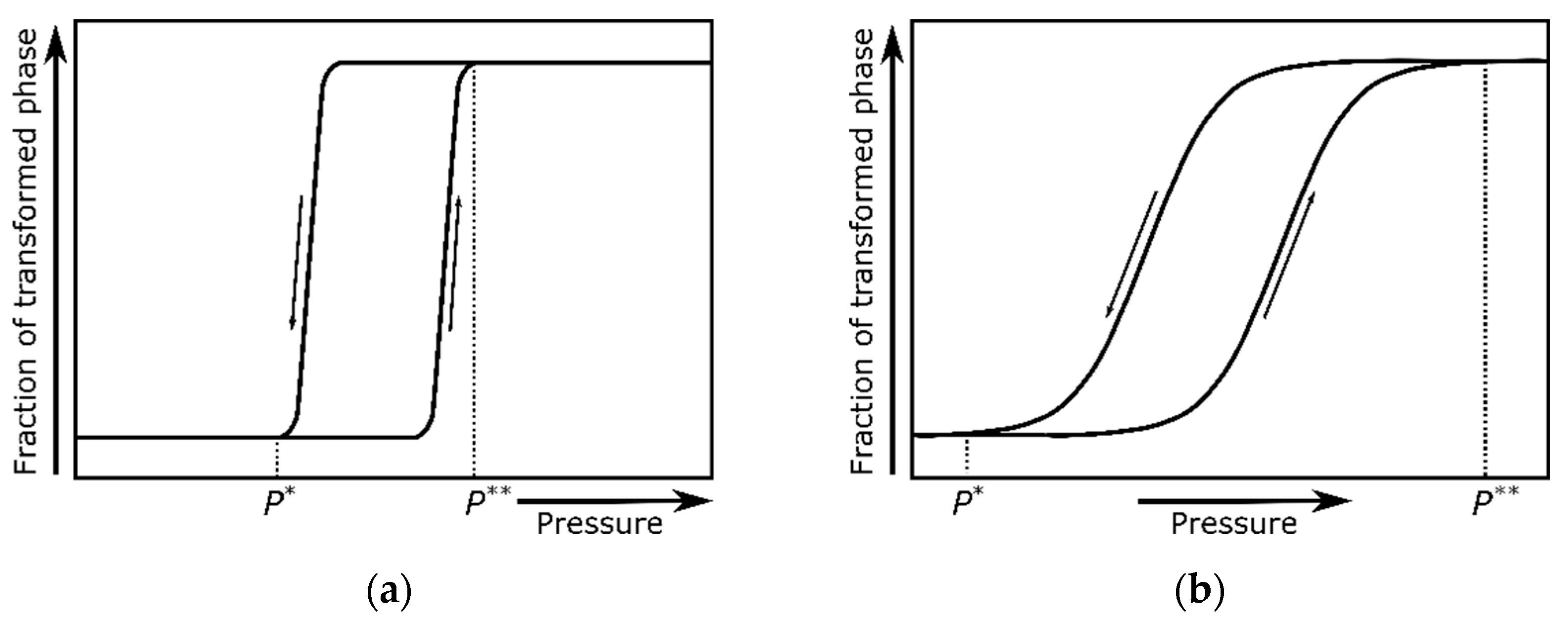
Furthermore, it has to be stressed that the solid-state first-order transitions proceed through the nucleation and growth of interfaces. If the kinetics of nucleation is much slower than the rate of the pressure (or temperature) change, then one can observe the phase coexistence, where the mass fraction between the two phases changes across the transformation [16]. If the crystal structures are not similar, and the change from one structure to the other involves the significant reorganization of the bonding scheme at the atomic level, then the energy barrier of nucleation may be considerable and the transformation rate sluggish. Moreover, many other factors (such as the pressure- or temperature-variation rate, sample microstructure, or sample environment) may affect this process. Figure 2 demonstrates the fraction of the transformed phase as a function of pressure in a pressure-induced first-order transition for different kinetic rates.

Moreover, many of the reported high-pressure datasets are collected on compression only. The reasons are varied but are often quite mundane: limited beamtime or technical obstacles (jammed diamond-anvil cell, plastic deformation of the gasket, failure of the diamonds). Therefore, the observed conditions at which the new phase begins to appear may be far away from the point where the Gibbs free energies of the two phases are equal. This discrepancy is even more severe in the ultrahigh-pressure regime.

To sum up, various generic features are associated with first-order transitions, such as metastability, phase coexistence, hysteresis, and their dependence on the path followed in the pressure–temperature space. All these factors can affect the shape of the experimentally determined phase-boundary lines and, consequently, the phase diagram.

Finally, one should be aware that the phase stability has different definitions. The phase is thermodynamically stable if it corresponds to the minimum of the thermodynamic potential at a given pressure and temperature with respect to the other phases. It is roughly consistent with the IUPAC definition of “stable” regarding the chemical stability: “As applied to chemical species, the term expresses a thermodynamic property, which is quantitatively measured by relative molar standard Gibbs energies. A chemical species A is more stable than its isomer B if Δ_rG° > 0 for the (real or hypothetical) reaction A → B under standard conditions” [17]. An immediate conclusion from this definition is that, at the given pressure and temperature, there is only one thermodynamically stable phase. At the same time, the other structures are metastable (i.e., thermodynamically unstable states that can be identified with the local minima on the potential-energy hypersurface and persist due to kinetic hindrance). A good general definition of metastability was provided by Tschoegl [18]: “When a thermodynamic system is in stable equilibrium, a perturbation will result only in small (virtual) departures from its original conditions and these will be restored upon removal of the cause of the perturbation. A thermodynamic system is in unstable equilibrium if even a small perturbation will result in large, irreversible changes in its conditions. A system in metastable equilibrium will act as one in stable equilibrium if perturbed by a small perturbation but will not return to its initial conditions upon a large perturbation.”

Under equilibrium conditions, a crystal is dynamically stable (or vibrationally stable; these terms are synonymous) if its potential energy always increases for any combination of atomic displacements; hence, all of the atoms are trapped within the local energy minima. In the harmonic approximation, this corresponds to the real and positive phonon frequencies of all the phonon modes [19]. The presence of imaginary (negative) frequencies of vibration at reciprocal lattice vectors in the Brillouin zone testifies to the dynamic instability.

A crystal is mechanically stable (or elastically stable; synonymous terms) if it fulfills Born’s stability criteria, which were formulated for the first time in his 1940 paper [20]. In the harmonic approximation (i.e., for an unstressed material at zero pressure), the second-order elastic stiffness tensor (C) is defined as:

$$C_{ij}=\frac{1}{V_0}\left(\frac{{\partial }^{2}E}{\partial {\epsilon }_i\partial {\epsilon }_j}\right),$$

(3)

where E is the elastic energy of the crystal, V₀ is its equilibrium volume, ε_i, and ε_j are the components of the strain tensor, and C_ij are the elastic constants (i.e., the elements of the elastic tensor). The elastic energy of a crystal is quadratic with applied strains, as follows:

$$E=E_0+\frac{V_0}{2}{\displaystyle \sum }_{i=1}^6{\displaystyle \sum }_{j=1}^6{C}_{ij}{\epsilon }_i{\epsilon }_j.$$

(4)

According to the Born mechanical (elastic)-stability criterion, the crystal is mechanically (elastically) stable if the elastic energy is always positive. This corresponds to the requirement that the tensor (C) is positive definite, or equivalently, that all the eigenvalues of the C are positive. In a general case, the symmetric 6 × 6 s-order elastic stiffness tensor (C) contains 21 independent elements. While a more detailed analysis is beyond the scope of this paper, the interested reader is referred to the comprehensive article of Mouhat and Coudert [21], who generalized the necessary and sufficient Born mechanical-stability conditions for all crystal classes. It should be emphasized that the mechanical (elastic)-stability conditions can be generalized to systems under an arbitrary external load (σ) by introducing an elastic stiffness tensor (B) under load. The applied external stress is often a game-changing factor for the phase stability. If a system is mechanically unstable but dynamically stable under given conditions, then this may indicate a thermodynamically metastable state.

The definitions of dynamic and mechanical stability refer to different physical variables and are therefore independent of each other. For example, scandium carbide (ScC) was found to be mechanically stable, but dynamically unstable [22], while the bcc titanium structure is mechanically unstable, but dynamically stable [23].

4. Case Studies

The following examples will illustrate a variety of issues and concerns regarding the literature phase diagrams. Questions about their conformity to the universally accepted ideal-phase-diagram definition will be discussed.

4.1. Stable or Metastable, That Is the Question

4.1.1. Chemical Elements

Chemical elements have been extensively studied under pressure since the pioneering works of Percy Bridgman at the beginning of the last century. Several monographs are entirely devoted to the phase diagrams of elements [24,25]. The systematic behavior of chemical elements over a range of pressures and temperatures was also illustrated graphically in a specific form of the periodic table [26]. Despite the expected simplicity, designing phase diagrams of elements can pose a real challenge.

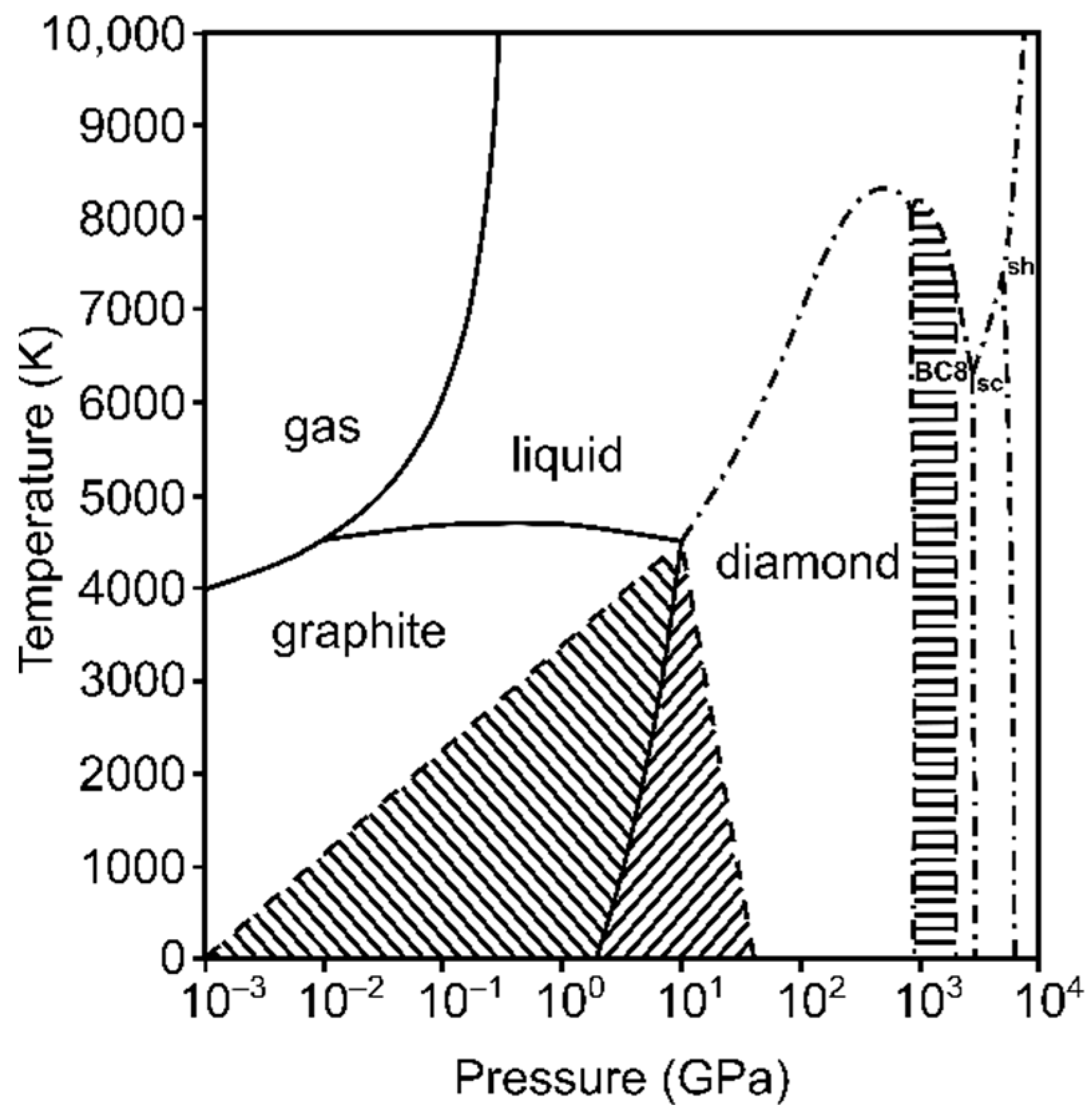
Carbon is arguably the element with the highest known number of chemical compounds due to its ability to bind covalently with other carbon atoms and form extended structures. It is also a chemical element with an overwhelming number of predicted crystal forms; the most recent release of the comprehensive Samara Carbon Allotrope Database (SACADA) contains 524 allotropes [27,28]. This complexity is not reflected in the experimental phase diagram of carbon [8,29,30,31,32], which contains only two experimentally determined solid phases, graphite and diamond, and other predicted phases, still not confirmed in experiments (see Figure 3). The first-order graphite ⇄ diamond phase transition has a high energy barrier, and the room-temperature compression of graphite does not yield diamond, but another three-dimensional metastable structure, in which chemical bonds between the neighboring graphene sheets are formed: the monoclinic M-carbon [33]. As expected, the kinetic barrier between the phases is lowered with the increase in temperature. On the one hand, synthetic laboratory-grown diamonds are produced at the pressure of ~5 GPa and a temperature of ~1800 K. On the other hand, the back transformation of diamond to graphite is kinetically hindered at room temperature and atmospheric pressure; hence, “diamonds are forever.” Fullerenes and nanotubes, which are famous families of carbon allotropes, are not found in the phase diagram of carbon because they are metastable under any P,T conditions with respect to graphite or diamond. Another well-known carbon allotrope, lonsdaleite, or the so-called “hexagonal diamond,” is not a separate phase but actually adopts a stacking-disordered diamond structure [34,35]. Hypothetical superdense carbon allotropes, some of them calculated to be thermodynamically stable in the terapascal regime, have been included in predicted phase diagrams of carbon [31,36,37]. However, a recent study on the ramp compression of diamond to 2 TPa demonstrates that the transition to stable dense allotropes is kinetically arrested due to a high energy barrier, similar to the hindered graphite ⇄ diamond transition in the modest-pressure range [32].

As mentioned above, the experimental determination of phase boundaries may be affected by numerous factors. A striking example is the phase transitions in lithium, where quantum and isotope effects play a crucial role in shaping its phase diagram [38]. It was known from earlier studies [39,40,41] that, upon cooling below ~77 K at atmospheric pressure, bcc ⁷Li transforms to a rhombohedral close-packed α-Sm-like 9R structure (space group $R\overline{3}m$), which, for a long time, was regarded as the ground state of lithium [40,41]. Careful selection of the pressure–temperature pathway (pressure-induced bcc → fcc transition at room temperature, followed by cooling to 20 K and subsequent decompression along the T = 20 K isotherm) helped to circumvent the bcc → 9R transition and facilitated the establishment of the actual ground state of the element, which is the fcc phase. By a prudent choice of words, the authors prevented ambiguities: while presenting the metastable 9R state on P–T charts, they entitled the figure “Observed stable and metastable crystal structures of ⁶Li and ⁷Li measured along the identified P–T paths”, avoiding the term “phase diagram” [38].

Another interesting case is phosphorous, where two textbook examples of allotropes, white and red phosphorous, are thermodynamically metastable under any P–T conditions and are missing in the phase diagram [42]. Black phosphorous, a ground-state structure built of corrugated layers of covalently bonded atoms, was synthesized for the first time by Percy Bridgman in 1914 by heating the white modification at high pressure [43]. It was one of the first spectacular achievements of high-pressure research. This form exhibits an interesting phenomenon of layer destabilization upon heating [44], although no other stable crystal phase was revealed in this experiment.

As already mentioned, the mechanical stability of the crystal can be tuned by the external stress. For example, first-principles calculations and stability analysis suggest that diamond becomes mechanically unstable when the difference between the radial- and axial-stress components exceeds 200 GPa [45]. In his review article, Levitas distinguished three types of phase transitions at high pressure: pressure-induced, stress-induced, and strain-induced transformations [46], and he described the differences between them in the following manner: “In most cases nucleation of the product phase occurs heterogeneously at some defects (dislocations, grain and twin boundaries), which produce a concentration of the stress tensor and/or provide some initial surface energy. Temperature-induced transformations nucleate predominantly at pre-existing defects without stresses at the specimen surface. Similarly, pressure-induced transformations occur mostly by nucleation at the same pre-existing defects under action of external hydrostatic pressure. Stress-induced transformations occur at the same defects when external nonhydrostatic stresses do not exceed the macroscopic yield strength in compression σ_y. If the phase transformations take place during plastic deformations they are classified as strain-induced transformations. They occur by nucleation at new defects generated during plastic deformation”. The effects of uniaxial stress on the phase-transition onset, hysteresis, and phase-coexistence range were demonstrated experimentally for the α ⇄ ε transition of iron [47] and the α ⇄ ω transition of titanium [48], employing various pressure-transmitting media.

4.1.2. Chemical Compounds

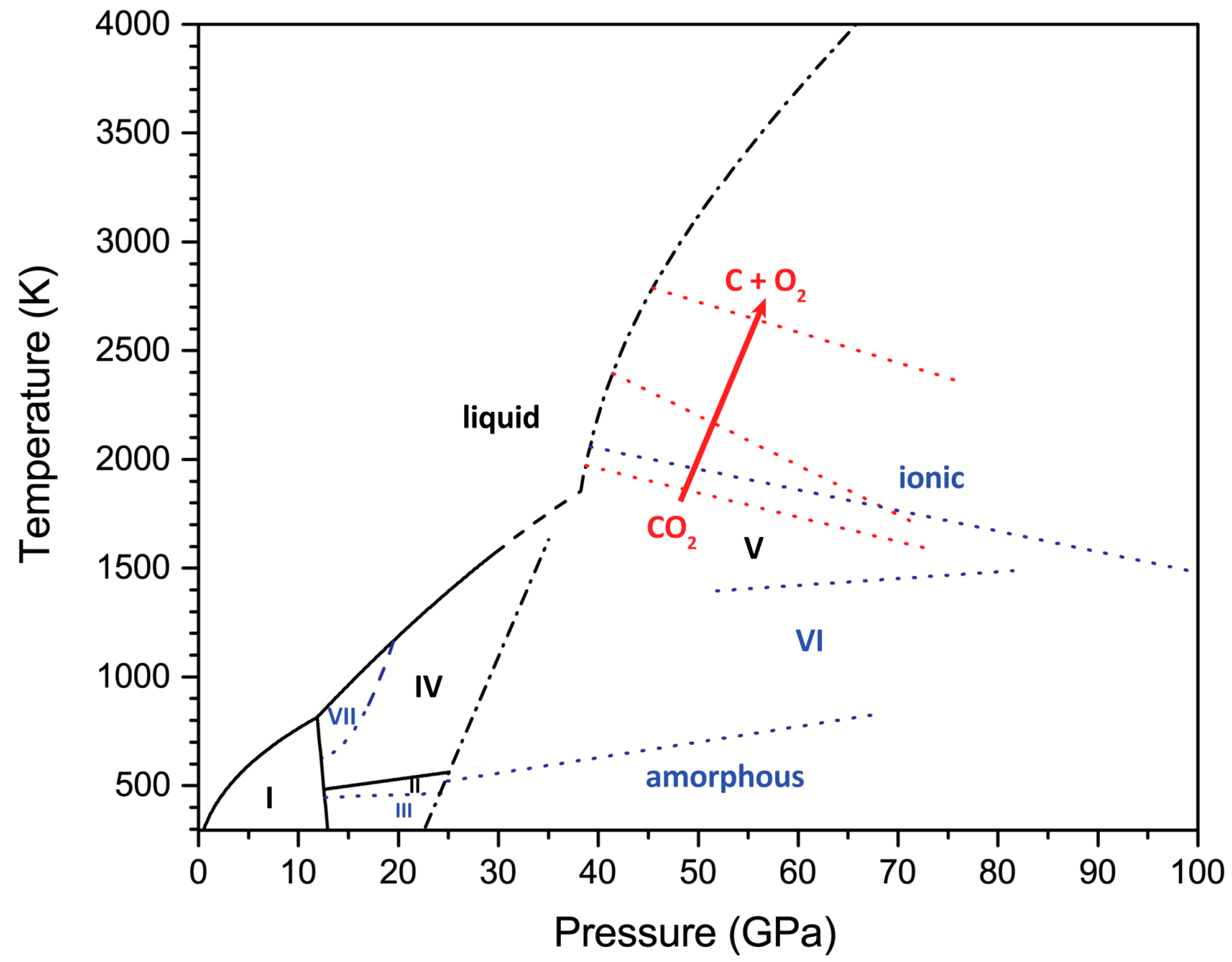
Chemical compounds exhibit a higher degree of complexity. The P–T phase diagrams are determined for all the phases with the same net stoichiometry (constant empirical formula). Even for the simplest cases, there are many contradictory results, which have stirred major controversies. One of the examples is carbon dioxide (CO₂), which, despite the simple stoichiometry, has quite a complex phase diagram that consists of several crystalline molecular polymorphs below ~35 GPa. Above this pressure, in laser-heated diamond-anvil-cell experiments, they transform to a polymeric tetragonal crystal phase, which is named CO₂-V, which can be described as a network of fourfold coordinated carbon atoms interconnected by oxygen bridges [49,50]. The substantial kinetic barrier that results from the reconstruction of the bonding scheme may preclude the formation of this phase, leading to the quenching of metastable states in the stability field of CO₂-V. Indeed, other extended covalent (CO₂-VI [51]) and even ionic (i-CO₂ [52]) structures of CO₂ have been suggested in experimental studies of CO₂ in the nonmolecular P–T regime. Recent reports that extend the pressure range beyond 100 GPa [53] and that employ in situ high-pressure–high-temperature (HP–HT) X-ray diffraction [54] confirmed that CO₂-V is the only stable modification of carbon dioxide at P > 35 GPa. Moreover, a previously reported dissociation of CO₂ to elements [55,56,57] was not observed, even in long laser-heating cycles up to a pressure above 100 GPa and T = 6200 K [54]. The P–T diagram of CO₂ showing the relationships between the equilibrium crystal phases and nonequilibrium states is illustrated in Figure 4. Please note that the position of the so-called kinetic transition lines may depend strongly on the pressure- and temperature-change rate and the P–T pathway.

The above example refers to a simple system that consists of two chemical elements. In principle, the vast majority of the materials are metastable, including almost all the organic compounds, as reflected, for example, in the description of the methodology of the constrained-evolutionary-algorithm calculations by Zhu et al. [64]: “Most of the molecular compounds are thermodynamically less stable than the simpler molecular compounds from which they can be obtained (such as H₂O, CO₂, CH₄, NH₃). This means that a fully unconstrained global optimization approach in many cases will produce a mixture of these simple molecules”. This statement falls squarely into the category of chemical stability and supports the expectation that the decomposition of complex molecules into a mixture of simpler structures is thermodynamically preferred; hence, such compounds are chemically metastable. Because the rate of transition is very often so slow (the energetic barrier is so high) that the transition to the thermodynamic ground state is practically not observed, and the shelf lives of many molecular compounds are in a timescale of years, the P–T diagrams of most of them (such as, e.g., paracetamol [65]) do not conform to the ideal-phase-diagram definition. Indeed, as Brazhkin noted in his viewpoint article [66]: “the objects of the physics of condensed media are primarily the equilibrium states of substances with metastable phases viewed as an exception, while in chemistry the overwhelming majority of organic substances under investigation are metastable. It turns out that at normal pressure many simple molecular compounds based on light elements (…) are metastable substances too, i.e., they do not match the Gibbs free energy minimum for a given atomic chemical composition. (…) Actually almost all so-called ‘phase diagrams’ of molecular substances in the reference books are in fact transitional diagrams (…)”. Such transitional diagrams are useful tools for analyzing molecular systems. In many organic compounds, the upper P–T limit of the metastability range of the molecular state is not a melting curve but a chemical-stability boundary, above which decomposition, polymerization, or pyrolysis is observed [67,68].

It is worth mentioning that the transformations between constrained metastable states have most of the features of phase transitions. In particular, the transition point in molecular solids can depend on factors such as the pressure-transmitting medium [69], nonhydrostatic conditions [70], and so on, affecting the shape of the associated transitional diagrams.

Lastly, it should be noted that, in the computational structure predictions of chemical compounds, the idea of the so-called convex hull is widely employed to predict stable phases. In the simplest case, for a binary AB system at zero temperature and zero pressure, it shows the enthalpy of formation (ΔH_F), plotted against the A:B molar ratio, represented on a linear segment between the pure A and B elements (unary phases) as the endmembers (composition–energy hull) [71]. Convex hulls contain only thermodynamically stable phases with the lowest possible formation energy for a given composition. Most frequently, these phases correspond to stoichiometric compounds that are characterized by the simplest whole-number A:B ratios. This idea can be extended to more complex systems and more dimensions: ternary systems are represented graphically in an equilateral triangle, quaternary systems in a tetrahedron, and so forth. Pressure can be included by adding volume as a parameter (composition–volume–energy hull) [71]. This concept can be helpful in the quest for new materials under high pressure [72], and even ones as complicated as the H–C–N–O quaternary system [73]. While the convex hulls cannot be directly rendered into P–T phase diagrams (mostly due to the difficulties related to accounting for temperature effects and creating a composition–volume–temperature–energy hull), a quick glimpse at a hull allows us to answer the question of whether the phase is stable towards decomposition into the constituent elements or other compounds with different stoichiometry by comparing their ΔH_F under the given thermodynamic conditions.

4.2. Pressure-Induced Amorphization, Glassy States, and Liquid–Liquid Transitions

Pressure-induced amorphization is a ubiquitous phenomenon that is observed as crystalline solids are compressed beyond their stability range under specific conditions (fast compression rate, low temperature) that hamper the expected crystal-to-crystal phase transition [74,75]. Amorphization can also occur upon the decompression of high-density phases. It can be associated with a chemical reaction; for example, at a moderate temperature (up to 680 K), molecular CO₂ starts to polymerize, forming amorphous carbonia glass [76], which is a chemically distinct species that contains carbon in threefold and fourfold coordination (see Figure 4). This transformation occurs when the temperature is too low to initiate and complete the phase transition to the thermodynamically stable CO₂-V crystal phase.

As McMillan and Wilding noted [75]: “Polyamorphic transformations between different amorphous “phases” that appear to mimic crystalline phase transitions also occur as a function of variables such as pressure (P) or temperature (T). Because glasses and other amorphous materials are not in internal thermodynamic equilibrium, such analogies must be made with care, however”. Indeed, glasses are not phases but are kinetically trapped metastable states (even if one can plot boundaries between the glassy states), and they shall not be present in the phase diagrams. For instance, the formation of amorphous ice results from the sluggish transition kinetics and can be overcome if the compression rate is very slow [77]. In this regard, one can plot a phase diagram of ice reporting the crystalline phases and a transitional P–T diagram revealing amorphous states (with boundaries between low-density amorphous, high-density amorphous, and very-high-density amorphous ice). Presenting “mixed” plots that comprise both stable and metastable states is also possible [78], but they have to be presented with appropriate comments to avoid any ambiguities.

Phase transitions in liquids are a different subject because they pertain to the state, which corresponds to the energy minimum in the P–T range beyond the melting curve. First-order liquid–liquid phase transitions usually occur between the states that are characterized by different local structures and short-range bonding schemes [75]. Examples are transitions in phosphorus between the low-density-liquid (LDL) phase consisting of discrete P₄ molecules and the polymeric high-density liquid (HDL) [79], or between the LDL and HDL phases of sulfur [80]. In the latter case, the phase-boundary line between the LDL and HDL ends with a critical point, which was a first experimental observation of a critical point in liquid–liquid phase transitions.

4.3. Critical Points and Supercritical States

As per the definition, in a phase diagram of a pure substance, liquid and gas are undistinguishable beyond the liquid–vapor critical point and constitute a single fluid phase. However, boundary lines that delimit the gas-like and liquid-like states of supercritical fluid can be noted in some instances. These boundaries do not correspond to classical phase transitions but can be revealed in experimental studies (e.g., investigating sound velocity in supercritical fluid argon reveals the so-called Widom line) [81].

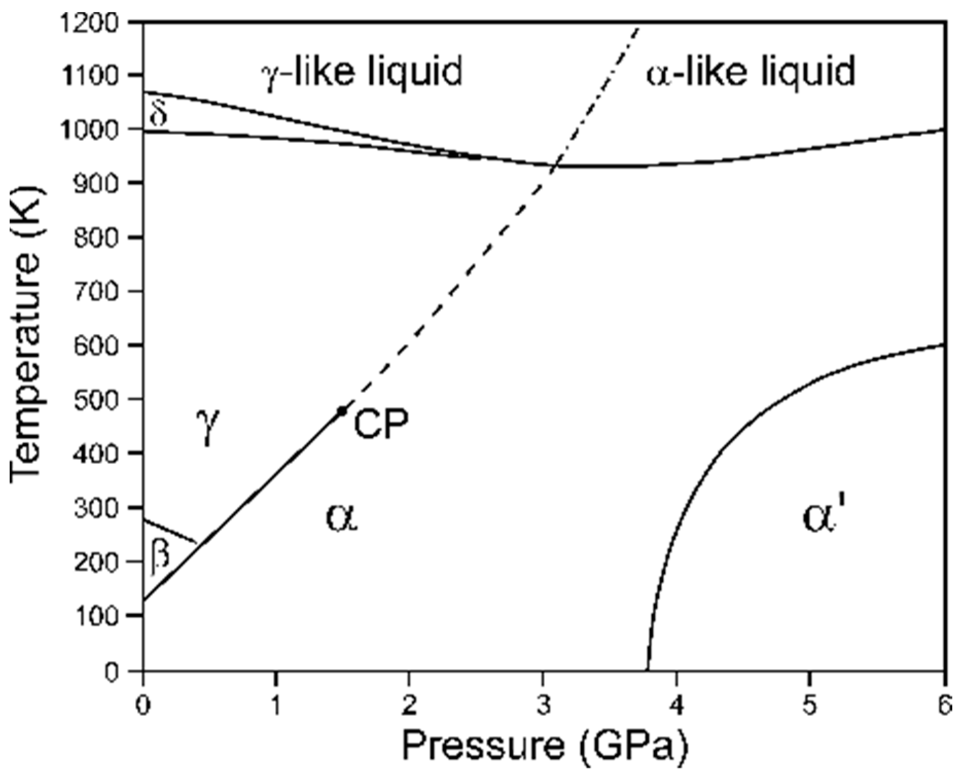
Critical points can also be observed at the end of the phase-boundary lines between the liquid states (e.g., in sulfur [80]). In solid phases, they are rare, primarily due to symmetry requirements. Usually a solid–solid phase-boundary line is intercepted by other phase boundaries or runs to infinity. One of the notable exceptions is the α ⇄ γ phase transition in cerium discovered by Percy Bridgman in 1927 [82], which has been intensively studied ever since [83]. Both phases share the same space-group symmetry (Fm-3m), and the observed first-order transition of electronic origin [84] is associated with a substantial volume collapse, which decreases with the pressure and temperature rise along the phase-boundary line, and eventually vanishes at the critical point. Interestingly, upon the extension of the α–γ phase boundary, no evidence of a second-order phase transition is found, but a minimum in the isothermal bulk modulus in the function of pressure is observed to the highest experimentally achieved temperature [85]. The P–V compression data revealed in the radiography study indicated that, at the extrapolation of the α–γ coexistence line to the liquid-state regime, the P(V) isotherm shows an inflection point, which indicates a plausible liquid–liquid phase transition [86] (see Figure 5).

4.4. Nonequilibrium Studies and Dynamic P–T Diagrams

The advent of dynamic-compression techniques has enabled experimental studies of matter under P–T conditions that are unattainable in static studies, and that allow for a reinvestigation of the previous reports with a new method. In shock-compressed silicon, the observed onset of phase transitions is lower than in similar static experiments [88]. In shock-compressed antimony, a similar lowering of the transition pressure is observed and an additional structure, not existing under “static” (i.e., very slow) compression, is revealed [89]. Some authors report the “dynamic phase diagrams” and speculate about the “modification of the phase diagram” of studied materials. However, it has to be emphasized in the strongest possible terms that dynamic P–T charts correspond to nonequilibrium conditions and cannot be regarded as phase diagrams in light of the ideal-phase-diagram definition. A perfect illustration of this fact is the accurate determination of phase-transition pressures in bismuth in a broad compression-rate range (10⁻²–10³ GPa/s) using a dynamic diamond-anvil cell [90]. The variation in the transition pressure of the Bi-III ⇄ Bi-V transition can actually be determined as a function of the compression rate. Similar relations can be observed in compression-rate-dependent transitional diagrams of organic compounds (e.g., L-serine) [91]. Such phenomena are therefore relatively frequent, and there is no single “dynamic phase diagram” for a given system, but a continuum of P–T diagrams, where the compression rate is an additional variable. One should also consider that, in dynamic experimental studies, many other factors can effectively tune the observed phase boundaries (such as the sample microstructure and environment (see, e.g., the differences between the runs on powder and foil bismuth, or the experiments on bismuth surrounded by neon versus those performed without a pressure-transmitting medium [90])). Finally, it must be taken into account that nonequilibrium processes can lead to the kinetic stabilization of metastable states. This refers to the definition of a transitional P–T diagram and the difference between dynamic and transitional diagrams, as formulated in the glossary of terms (Section 2 of this article). As the timescale is the principal and perhaps even the only basis for distinguishing these two terms, with no quantitative threshold, the criterion of discrimination is therefore purely discretionary. Hence, I am inclined to believe that only one of these terms should be officially recommended. In this regard, I would prefer to use the term transitional rather than dynamic, as virtually any variable-pressure study is de facto dynamic, although some experiments can appear as quasistatic.

5. Conclusions and Call for Actions

Phase diagrams are simple visual representations that communicate key data related to the state of matter under varied thermodynamic conditions. Their focus and clarity make them understandable and accessible, even at the undergraduate level [92]. However, the notion of a phase diagram needs to be better defined. After running through all these examples, it is time to go back to the opening quotation from Ogden and Richards’ “The Meaning of Meaning” and reflect on the status quo. I think the community should settle the terms and find a common language to avoid further misunderstandings. For many, “phase diagram” is a buzzword that automatically springs to mind when referring to any pressure–temperature chart. Do not worry, there is no scientific police that hounds for the misuse of the phase-diagram definition. Let me conclude with some closing remarks, which may serve as a starting point for a further discussion. It would be perfect if this debate resulted in the reaching of a consensus on the most significant working definitions and the issuing of official recommendations by international scientific organizations, such as IUPAC, IUCr, and AIRAPT [93]. To catalyze and facilitate the exchange of ideas, in

Table 1. The issues associated with the presentation of phase diagrams and suggestions for improvements.

Issues	Potential Solutions
The definition of an ideal phase diagram is quite limited to the elements and simplest chemical compounds. P–T plots of more complex systems, often reported as phase diagrams, are transitional P–T diagrams or “metastable phase diagrams.” Even when regarding only chemical elements, one should be extremely careful with wording 1.	It should be acknowledged that a presented phase diagram is the best estimate of the ideal phase diagram based on experimental and theoretical constraints. At the base of the wording phase diagram lies the assumption that: (1) the presented states are thermodynamically stable phases; (2) the described situation is as close to the thermodynamic equilibrium as possible.
There is no harm in presenting nonequilibrium P–T diagrams if only experimental conditions are described in detail. Reporting nonequilibrium states (in particular, amorphous glasses) incorporated within an equilibrium phase diagram may be utterly confusing when not described appropriately.	Transitional P–T diagrams that include nonequilibrium states can be reported only if additional information is indicated and commented on in the legend and caption. The careful description is substantial, especially to distinguish between the thermodynamically stable phases and kinetically trapped metastable states. In such plots, the position of the kinetic transition lines may strongly depend on the experimental conditions and the P–T pathway. Such P–T diagrams should not be referred to as phase diagrams.
Undoubtedly, discovering new stable phases is of paramount importance in condensed-matter chemistry and physics. However, some literature P–T plots report numerous “phases” that appear to be metastable states after a more thorough investigation. Articles containing the catchphrase “we revised the phase diagram of…” make little sense if the authors of previous studies understand the term differently. To paraphrase Occam’s razor, supposedly stable phases should not be multiplied beyond necessity.	The reported phases should conform to the definition of a thermodynamically stable phase. Under no circumstances can a claim of the revision of a phase diagram be accepted if the reported states are metastable.
Some specific boundary lines (such as liquid–liquid-transition curves and Widom lines) and critical points may appear in a phase diagram or transitional P–T diagram. It is essential, however, to characterize them well in the plot or figure caption.	All the elements of the reported diagrams should be communicated in a clear and unambiguous fashion.
Dynamic P–T diagrams (based on the results of compression experiments) do not comply with the phase-diagram definition, as they do not correspond to an equilibrium state. The compression rate can shift phase boundaries and, as such, may be regarded as an additional variable, but one has to bear in mind that many other factors can also influence the boundary lines under nonequilibrium conditions. Having said that, an ideally static P–T diagram does not exist, as any compression and decompression is a time-dependent process. The crucial factor is, therefore, the ratio between the rate of transformation and the rate of pressurization or depressurization.	The terms dynamic P–T diagram and transitional P–T diagrams are almost synonymous; however, the second one is used more often to report the results of quasistatic compression experiments. As there is no universally accepted compression-rate threshold that unequivocally distinguishes these two notions, the term dynamic P–T diagram appears to be redundant.

¹ For example, a transitional P–T diagram of buckminsterfullerene (C₆₀) is not a phase diagram of carbon, and a transitional P–T diagram of ozone (O₃) is not a phase diagram of oxygen, and so on.

, I present some preliminary suggestions and measures to tackle the fundamental problems in the current presentation of phase diagrams, providing insight into issues and potential solutions.

References

- Ogden, C.K.; Richards, I.A. The Meaning of Meaning: A Study of the Influence of Language upon Thought and of the Science of Symbolism, 1st ed.; Routledge & Kegan Paul: London, UK, 1923. [Google Scholar]
- IUPAC Gold Book. Available online: https://goldbook.iupac.org (accessed on 25 July 2022).
- IUCr Online Dictionary of Crystallography. Available online: https://dictionary.iucr.org (accessed on 25 July 2022).
- Grochala, W. Pressure-induced phase transitions. In Chemical Reactivity in Confined Systems: Theory, Modelling and Applications, 1st ed.; Chattaraj, P.K., Chakraborty, A., Eds.; Wiley: Hoboken, NJ, USA, 2021; pp. 25–47. [Google Scholar]
- Oxford English Dictionary Online. Available online: https://www.oed.com (accessed on 25 July 2022).
- Luo, K.; Liu, B.; Hu, W.; Dong, X.; Wang, Y.; Huang, Q.; Gao, Y.; Sun, L.; Zhao, Z.; Wu, Y.; et al. Coherent interfaces with mixed hybridization govern direct transformation from graphite to diamond. Nature 2022, 607, 486–491. [Google Scholar] [CrossRef] [PubMed]
- Turnbull, R.; Hanfland, M.; Binns, J.; Martinez-Canales, M.; Frost, M.; Marqués, M.; Howie, R.T.; Gregoryanz, E. Unusually complex phase of dense nitrogen at extreme conditions. Nat. Commun. 2018, 9, 4717. [Google Scholar] [CrossRef] [PubMed]
- Bundy, F.P.; Bassett, W.A.; Weathers, M.S.; Hemley, R.J.; Mao, H.K.; Goncharov, A.F. The pressure-temperature phase and transformation diagram for carbon; updated through 1994. Carbon 1996, 34, 141–153. [Google Scholar] [CrossRef]
- Ehrenfest, P. Phasenumwandlungen im ueblichen und erweiterten Sinn, Classifiziert nach dem Entsprechenden Singularitaeten des Thermodynamischen Potentiales; N. V. Noord-Hollandsche Uitgevers Maatschappij: Amsterdam, The Netherlands, 1933; Volume 36, pp. 153–157. [Google Scholar]
- Jaeger, G. The Ehrenfest classification of phase transitions: Introduction and evolution. Arch. Hist. Exact Sci. 1998, 53, 51–81. [Google Scholar] [CrossRef]
- Sauer, T. A look back at the Ehrenfest classification. Translation and commentary of Ehrenfest’s 1933 paper introducing the notion of phase transitions of different order. Eur. Phys. J. Spec. Topics 2017, 226, 539–549. [Google Scholar] [CrossRef] [Green Version]
- Landau, L.D.; Lifshitz, E.M. Statistical Physics, 3rd ed.; Pergamon Press: Oxford, UK, 1980. [Google Scholar]
- Frenkel, J. Kinetic Theory of Liquids, 1st ed.; Clarendon Press: Oxford, UK, 1946. [Google Scholar]
- Turnbull, D. Phase changes. In Solid State Physics, 1st ed.; Seitz, F., Turnbull, D., Eds.; Academic Press: New York, NY, USA, 1956; Volume 3, pp. 225–306. [Google Scholar]
- Dash, J.G. Melting from one to two to three dimensions. Contemp. Phys. 2002, 43, 427–436. [Google Scholar] [CrossRef]
- Mnyuk, Y. Mechanism and kinetics of phase transitions and other reactions in solids. Am. J. Condens. Matter Phys. 2013, 3, 89–103. [Google Scholar]
- Muller, P. Glossary of terms used in physical organic chemistry (IUPAC Recommendations 1994). Pure Appl. Chem. 1994, 66, 1077–1184. [Google Scholar] [CrossRef] [Green Version]
- Tschoegl, N.W. Fundamentals of Equilibrium and Steady-State Thermodynamics, 1st ed.; Elsevier: Amsterdam, The Netherlands, 2000. [Google Scholar]
- Wallace, D.C. Thermodynamics of Crystals, 1st ed.; Wiley: New York, NY, USA, 1972. [Google Scholar]
- Born, M. On the stability of crystal lattices. I. Math. Proc. Cambridge Philos. Soc. 1940, 36, 160–172. [Google Scholar] [CrossRef]
- Mouhat, F.; Coudert, F.-X. Necessary and sufficient elastic stability conditions in various crystal systems. Phys. Rev. B 2014, 90, 224104. [Google Scholar] [CrossRef] [Green Version]
- Abu-Jafar, M.S.; Leonhardi, V.; Jaradat, R.; Mousa, A.A.; Al-Qaisi, S.; Mahmoud, N.T.; Bassalat, A.; Khenata, R.; Bouhemadou, A. Structural, electronic, mechanical, and dynamical properties of scandium carbide. Results Phys. 2021, 21, 103804. [Google Scholar] [CrossRef]
- Kadkhodaei, S.; Hong, Q.-J.; van de Walle, A. Free energy calculation of mechanically unstable but dynamically stabilized bcc titanium. Phys. Rev. B 2017, 95, 064101. [Google Scholar] [CrossRef] [Green Version]
- Young, D.A. Phase Diagrams of the Elements, 1st ed.; University of California Press: Berkeley, CA, USA, 1991. [Google Scholar]
- Tonkov, E.Y.; Ponyatovsky, E.G. Phase Transformations of the Elements Under High Pressure, 1st ed.; CRC Press: Boca Raton, FL, USA, 2005. [Google Scholar]
- Holzapfel, W.B. Structures of the elements—Crystallography and art. Acta Crystallogr. B 2014, 70, 429–435. [Google Scholar] [CrossRef] [PubMed]
- SACADA—Samara Carbon Allotrope Database. Available online: https://www.sacada.info (accessed on 25 July 2022).
- Hoffmann, R.; Kabanov, A.A.; Golov, A.A.; Proserpio, D.M. Homo Citans and Carbon Allotropes: For an Ethics of Citation. Angew. Chem. Int. Ed. Engl. 2016, 55, 10962–10976. [Google Scholar] [CrossRef] [PubMed]
- Bundy, F.P. Pressure-temperature phase diagram of elemental carbon. Phys. A Stat. Mech. Its Appl. 1989, 156, 169–178. [Google Scholar] [CrossRef]
- Zazula, J.M. On Graphite Transformations at High Temperature and Pressure Induced by Absorption of the LHC Beam; CERN-LHC-Project-Note-78/97; CERN: Geneva, Switzerland, 1997. [Google Scholar]
- Benedict, L.X.; Driver, K.P.; Hamel, S.; Militzer, B.; Qi, T.; Correa, A.A.; Saul, A.; Schwegler, E. Multiphase equation of state for carbon addressing high pressures and temperatures. Phys. Rev. B 2014, 89, 224109. [Google Scholar] [CrossRef] [Green Version]
- Lazicki, A.; McGonegle, D.; Rygg, J.R.; Braun, D.; Swift, D.C.; Gorman, M.G.; Smith, R.F.; Heighway, P.; Higginbotham, A.; Suggit, M.J.; et al. Metastability of diamond ramp-compressed to 2 terapascals. Nature 2021, 589, 532–535. [Google Scholar] [CrossRef]
- Wang, Y.; Panzik, J.E.; Kiefer, B.; Lee, K.K.M. Crystal structure of graphite under room-temperature compression and decompression. Sci. Rep. 2012, 2, 520. [Google Scholar] [CrossRef]
- Németh, P.; Garvie, L.A.J.; Aoki, T.; Natalia, D.; Dubrovinsky, L.; Buseck, P.R. Lonsdaleite is faulted and twinned cubic diamond and does not exist as a discrete material. Nat. Commun. 2014, 5, 5447. [Google Scholar] [CrossRef] [Green Version]
- Salzmann, C.G.; Murray, B.J.; Shephard, J.J. Extent of stacking disorder in diamond. Diam. Relat. Mater. 2015, 59, 69–72. [Google Scholar] [CrossRef] [Green Version]
- Correa, A.A.; Bonev, S.A.; Galli, G. Carbon under extreme conditions: Phase boundaries and electronic properties from first-principles theory. Proc. Natl. Acad. Sci. USA 2006, 103, 1204–1208. [Google Scholar] [CrossRef] [PubMed] [Green Version]
- Sun, J.; Klug, D.D.; Martoňák, R. Structural transformations in carbon under extreme pressure: Beyond diamond. J. Chem. Phys. 2009, 130, 194512. [Google Scholar] [CrossRef] [PubMed]
- Ackland, G.J.; Dunuwille, M.; Martinez-Canales, M.; Loa, I.; Zhang, R.; Sinogeikin, S.; Cai, W.; Deemyad, S. Quantum and isotope effects in lithium metal. Science 2017, 356, 1254–1259. [Google Scholar] [CrossRef] [PubMed] [Green Version]
- Barrett, C.S. A low temperature transformation in lithium. Phys. Rev. 1947, 72, 245. [Google Scholar] [CrossRef]
- Overhauser, A.W. Crystal structure of lithium at 4.2 K. Phys. Rev. Lett. 1984, 53, 64–65. [Google Scholar] [CrossRef]
- Smith, H.G. Martensitic phase transformation of single-crystal lithium from bcc to a 9R-related structure. Phys. Rev. Lett. 1987, 58, 1228–1231. [Google Scholar] [CrossRef]
- Scelta, D.; Baldassarre, A.; Serrano-Ruiz, M.; Dziubek, K.; Cairns, A.B.; Peruzzini, M.; Bini, R.; Ceppatelli, M. Interlayer bond formation in black phosphorus at high pressure. Angew. Chem. Int. Ed. Engl. 2017, 56, 14135–14140. [Google Scholar] [CrossRef]
- Bridgman, P.W. Two new modifications of phosphorus. J. Am. Chem. Soc. 1914, 36, 1344–1363. [Google Scholar] [CrossRef] [Green Version]
- Henry, L.; Svitlyk, V.; Mezouar, M.; Sifré, D.; Garbarino, G.; Ceppatelli, M.; Serrano-Ruiz, M.; Peruzzini, M.; Datchi, F. Anisotropic thermal expansion of black phosphorus from nanoscale dynamics of phosphorene layers. Nanoscale 2020, 12, 4491–4497. [Google Scholar] [CrossRef]
- Zhao, J.-J.; Scandolo, S.; Kohanoff, J.; Chiarotti, G.L.; Tosatti, E. Elasticity and mechanical instabilities of diamond at megabar stresses: Implications for diamond-anvil-cell research. Appl. Phys. Lett. 1999, 75, 487–488. [Google Scholar] [CrossRef]
- Levitas, V.I. High pressure phase transformations revisited. J. Phys. Condens. Matter 2018, 30, 163001. [Google Scholar] [CrossRef] [PubMed] [Green Version]
- Boehler, R.; von Bargen, N.; Chopelas, A. Melting, thermal expansion, and phase transitions of iron at high pressures. J. Geophys. Res. 1990, 95, 21731–21736. [Google Scholar] [CrossRef]
- Errandonea, D.; Meng, Y.; Somayazulu, M.; Häusermann, D. Pressure-induced α→ω transition in titanium metal: A systematic study of the effects of uniaxial stress. Phys. B Condens. Matter 2005, 355, 116–125. [Google Scholar] [CrossRef] [Green Version]
- Santoro, M.; Gorelli, F.A.; Bini, R.; Haines, J.; Cambon, O.; Levelut, C.; Montoya, J.A.; Scandolo, S. Partially collapsed cristobalite structure in the non molecular phase V in CO2. Proc. Natl. Acad. Sci. USA 2012, 109, 5176–5179. [Google Scholar] [CrossRef] [Green Version]
- Datchi, F.; Mallick, B.; Salamat, A.; Ninet, S. Structure of polymeric carbon dioxide CO2-V. Phys. Rev. Lett. 2012, 108, 125701. [Google Scholar] [CrossRef]
- Iota, V.; Yoo, C.-S.; Klepeis, J.-H.; Jenei, Z.; Evans, W.; Cynn, H. Six-fold coordinated carbon dioxide VI. Nat. Mater. 2007, 6, 34–38. [Google Scholar] [CrossRef]
- Yoo, C.-S.; Sengupta, A.; Kim, M. Carbon dioxide carbonates in the Earth’s mantle: Implications to the deep carbon cycle. Angew. Chem. Int. Ed. 2011, 50, 11219–11222. [Google Scholar] [CrossRef]
- Dziubek, K.F.; Ende, M.; Scelta, D.; Bini, R.; Mezouar, M.; Garbarino, G.; Miletich, R. Crystalline polymeric carbon dioxide stable at megabar pressures. Nat. Comm. 2018, 9, 3148. [Google Scholar] [CrossRef]
- Scelta, D.; Dziubek, K.F.; Ende, M.; Miletich, R.; Mezouar, M.; Garbarino, G.; Bini, R. Extending the stability field of polymeric carbon dioxide phase V beyond the Earth’s geotherm. Phys. Rev. Lett. 2021, 126, 065701. [Google Scholar] [CrossRef]
- Tschauner, O.; Mao, H.-k.; Hemley, R.J. New transformations of CO2 at high pressures and temperatures. Phys. Rev. Lett. 2001, 87, 075701. [Google Scholar] [CrossRef]
- Seto, Y.; Hamane, D.; Nagai, T.; Fujino, K. Fate of carbonates within oceanic plates subducted to the lower mantle, and a possible mechanism of diamond formation. Phys. Chem. Miner. 2008, 35, 223–229. [Google Scholar] [CrossRef]
- Litasov, K.D.; Goncharov, A.F.; Hemley, R.J. Crossover from melting to dissociation of CO2 under pressure: Implications for the lower mantle. Earth Planet. Sci. Lett. 2011, 309, 318–323. [Google Scholar] [CrossRef]
- Giordano, V.M.; Datchi, F.; Dewaele, A. Melting curve and fluid equation of state of carbon dioxide at high pressure and high temperature. J. Chem. Phys. 2006, 125, 054504. [Google Scholar] [CrossRef] [PubMed] [Green Version]
- Giordano, V.M.; Datchi, F. Molecular carbon dioxide at high pressure and high temperature. EPL 2007, 77, 46002. [Google Scholar] [CrossRef]
- Iota, V.; Yoo, C.S. Phase diagram of carbon dioxide: Evidence for a new associated phase. Phys. Rev. Lett. 2001, 86, 5922–5925. [Google Scholar] [CrossRef]
- Cogollo-Olivo, B.H.; Biswas, S.; Scandolo, S.; Montoya, J.A. Ab initio determination of the phase diagram of CO2 at high pressures and temperatures. Phys. Rev. Lett. 2020, 124, 095701. [Google Scholar] [CrossRef] [Green Version]
- Teweldeberhan, A.M.; Boates, B.; Bonev, S.A. CO2 in the mantle: Melting and solid-solid phase boundaries. Earth Planet. Sci. Lett. 2013, 373, 228–232. [Google Scholar] [CrossRef] [Green Version]
- Datchi, F.; Weck, G. X-ray crystallography of simple molecular solids up to megabar pressures: Application to solid oxygen and carbon dioxide. Z. Kristallogr. 2014, 229, 135–157. [Google Scholar] [CrossRef] [Green Version]
- Zhu, Q.; Oganov, A.R.; Glass, C.W.; Stokes, H.T. Constrained evolutionary algorithm for structure prediction of molecular crystals: Methodology and applications. Acta Crystallogr. B 2012, 68, 215–226. [Google Scholar] [CrossRef]
- Smith, S.J.; Montgomery, J.M.; Vohra, Y.K. High-pressure high-temperature phase diagram of organic crystal paracetamol. J. Phys. Condens. Matter 2016, 28, 035101. [Google Scholar] [CrossRef]
- Brazhkin, V.V. Metastable phases and ‘metastable’ phase diagrams. J. Phys. Condens. Matter 2006, 18, 9643–9650. [Google Scholar] [CrossRef]
- Ciabini, L.; Santoro, M.; Gorelli, F.A.; Bini, R.; Schettino, V.; Raugei, S. Triggering dynamics of the high-pressure benzene amorphization. Nat. Mater. 2006, 6, 39–43. [Google Scholar] [CrossRef] [PubMed]
- Dziubek, K.; Citroni, M.; Fanetti, S.; Cairns, A.B.; Bini, R. Synthesis of high-quality crystalline carbon nitride oxide by selectively driving the high-temperature instability of urea with pressure. J. Phys. Chem. C 2017, 121, 19872–19879. [Google Scholar] [CrossRef] [Green Version]
- Zakharov, B.A.; Seryotkin, Y.V.; Tumanov, N.A.; Paliwoda, D.; Hanfland, M.; Kurnosov, A.V.; Boldyreva, E.V. The role of fluids in high-pressure polymorphism of drugs: Different behaviour of β-chlorpropamide in different inert gas and liquid media. RSC Adv. 2016, 6, 92629–92637. [Google Scholar] [CrossRef] [Green Version]
- Guńka, P.A.; Olejniczak, A.; Fanetti, S.; Bini, R.; Collings, I.E.; Svitlyk, V.; Dziubek, K.F. Crystal structure and non-hydrostatic stress-induced phase transition of urotropine under high pressure. Chem. Eur. J. 2021, 27, 1094–1102. [Google Scholar] [CrossRef]
- Amsler, M.; Hegde, V.I.; Jacobsen, S.D.; Wolverton, C. Exploring the high-pressure materials genome. Phys. Rev. X 2018, 8, 041021. [Google Scholar] [CrossRef] [Green Version]
- Hilleke, K.P.; Bi, T.; Zurek, E. Materials under high pressure: A chemical perspective. Appl. Phys. A 2022, 128, 441. [Google Scholar] [CrossRef]
- Conway, L.J.; Pickard, C.J.; Hermann, A. Rules of formation of H–C–N–O compounds at high pressure and the fates of planetary ices. Proc. Natl. Acad. Sci. USA 2021, 118, e2026360118. [Google Scholar] [CrossRef]
- Machon, D.; Meersman, F.; Wilding, M.C.; Wilson, M.; McMillan, P.F. Pressure-induced amorphization and polyamorphism: Inorganic and biochemical systems. Prog. Mater. Sci. 2014, 61, 216–282. [Google Scholar] [CrossRef]
- McMillan, P.F.; Wilding, M.C. Polyamorphism and liquid–liquid phase transitions. In Encyclopedia of Glass Science, Technology, History, and Culture, 1st ed.; Richet, P., Ed.; Wiley: Hoboken, NJ, USA, 2021; Volume 1, pp. 359–370. [Google Scholar]
- Santoro, M.; Gorelli, F.A.; Bini, R.; Ruocco, G.; Scandolo, S.; Crichton, W.A. Amorphous silica-like carbon dioxide. Nature 2006, 441, 857–860. [Google Scholar] [CrossRef]
- Tulk, C.A.; Molaison, J.J.; Makhluf, A.R.; Manning, C.E.; Klug, D.D. Absence of amorphous forms when ice is compressed at low temperature. Nature 2019, 569, 542–545. [Google Scholar] [CrossRef] [PubMed]
- Amann-Winkel, K.; Böhmer, R.; Fujara, F.; Gainaru, C.; Geil, B.; Loerting, T. Colloquium: Water’s controversial glass transitions. Rev. Mod. Phys. 2016, 88, 011002. [Google Scholar] [CrossRef]
- Katayama, Y.; Inamura, Y.; Mizutani, T.; Yamakata, M.; Utsumi, W.; Shimomura, O. Macroscopic separation of dense fluid phase and liquid phase of phosphorus. Science 2004, 306, 848–851. [Google Scholar] [CrossRef]
- Henry, L.; Mezouar, M.; Garbarino, G.; Sifré, D.; Weck, G.; Datchi, F. Liquid–liquid transition and critical point in sulfur. Nature 2020, 584, 382–386. [Google Scholar] [CrossRef] [PubMed]
- Simeoni, G.G.; Bryk, T.; Gorelli, F.A.; Krisch, M.; Ruocco, G.; Santoro, M.; Scopigno, T. The Widom line as the crossover between liquid-like and gas-like behaviour in supercritical fluids. Nat. Phys. 2010, 6, 503–507. [Google Scholar] [CrossRef]
- Bridgman, P.W. The compressibility and pressure coefficient of resistance of ten elements. Proc. Am. Acad. Arts. Sci. 1927, 62, 207–226. [Google Scholar] [CrossRef]
- Decremps, F.; Belhadi, L.; Farber, D.L.; Moore, K.T.; Occelli, F.; Gauthier, M.; Polian, A.; Antonangeli, D.; Aracne-Ruddle, C.M.; Amadon, B. Diffusionless γ⇄α phase transition in polycrystalline and single-crystal cerium. Phys. Rev. Lett. 2011, 106, 065701. [Google Scholar] [CrossRef] [Green Version]
- Devaux, N.; Casula, M.; Decremps, F.; Sorella, S. Electronic origin of the volume collapse in cerium. Phys. Rev. B 2015, 91, 081101. [Google Scholar] [CrossRef] [Green Version]
- Lipp, M.J.; Jackson, D.; Cynn, H.; Aracne, C.; Evans, W.J.; McMahan, A.K. Thermal signatures of the Kondo volume collapse in cerium. Phys. Rev. Lett. 2008, 101, 165703. [Google Scholar] [CrossRef]
- Lipp, M.J.; Jenei, Z.; Ruddle, D.; Aracne-Ruddle, C.; Cynn, H.; Evans, W.J.; Kono, Y.; Kenney-Benson, C.; Park, C. Equation of state measurements by radiography provide evidence for a liquid-liquid phase transition in cerium. J. Phys. Conf. Ser. 2014, 500, 032011. [Google Scholar] [CrossRef] [Green Version]
- Munro, K.A.; Daisenberger, D.; MacLeod, S.G.; McGuire, S.; Loa, I.; Popescu, C.; Botella, P.; Errandonea, D.; McMahon, M.I. The high-pressure, high-temperature phase diagram of cerium. J. Phys. Condens. Matter 2020, 32, 335401. [Google Scholar] [CrossRef] [PubMed]
- McBride, E.E.; Krygier, A.; Ehnes, A.; Galtier, E.; Harmand, M.; Konôpková, Z.; Lee, H.J.; Liermann, H.-P.; Nagler, B.; Pelka, A.; et al. Phase transition lowering in dynamically compressed silicon. Nat. Phys. 2019, 15, 89–94. [Google Scholar] [CrossRef]
- Coleman, A.L.; Gorman, M.G.; Briggs, R.; McWilliams, R.S.; McGonegle, D.; Bolme, C.A.; Gleason, A.E.; Fratanduono, D.E.; Smith, R.F.; Galtier, E.; et al. Identification of phase transitions and metastability in dynamically compressed antimony using ultrafast X-ray diffraction. Phys. Rev. Lett. 2019, 122, 255704. [Google Scholar] [CrossRef] [PubMed] [Green Version]
- Husband, R.J.; O’Bannon, E.F.; Liermann, H.-P.; Lipp, M.J.; Méndez, A.S.J.; Konôpková, Z.; McBride, E.E.; Evans, W.J.; Jenei, Z. Compression-rate dependence of pressure-induced phase transitions in Bi. Sci. Rep. 2021, 11, 14859. [Google Scholar] [CrossRef] [PubMed]
- Fisch, M.; Lanza, A.; Boldyreva, E.; Macchi, P.; Casati, N. Kinetic control of high-pressure solid-state phase transitions: A Case Study on L-serine. J. Phys. Chem. C 2015, 119, 18611–18617. [Google Scholar] [CrossRef] [Green Version]
- Gramsch, S.A. A closer look at phase diagrams for the general chemistry course. J. Chem. Ed. 2000, 77, 718–723. [Google Scholar] [CrossRef]
- International Association for the Advancement of High Pressure Science and Technology (Association Internationale pour l’Avancement de la Recherche et de la Technologie aux Hautes Pressions). Available online: https://www.airapt.org (accessed on 20 July 2022).
Figure 1.
Thermodynamic-potential surfaces for two phases, I and II, as functions of pressure and temperature. The projection onto the P–T plane represents the phase diagram, whereas the line of intersection of the two surfaces corresponds to the I–II-phase-transition boundary. Black dots represent the stages of experimental isothermal compression or decompression routes. P* and P** define the limits of the metastability range, while Ptrans denotes the equilibrium transition pressure.
Figure 2.
The fraction of the transformed phase as a function of pressure representing a relatively fast (a) and slow (b) rate of interconversion. P* and P** mark the lower and upper bounds of the phase coexistence range.
Figure 3.
The simplified transitional P–T diagram of carbon, after [8,29,30,31,32]. Note the logarithmic scale for pressure. The left and right hashed areas correspond to the regions of metastability of graphite and diamond, with metastability boundaries marked as dashed lines. Dash-dotted contours delineate the calculated melting curve of diamond and stability fields of the predicted BC8, simple cubic (sc), and simple hexagonal (sh) phases [31], which have been never confirmed experimentally. The horizontal hashed area demonstrates the persistence of diamond in a ramp-compression experiment up to 2 TPa [32] within the predicted thermodynamic stability field of the BC8 phase. While the kinetics of the graphite ⇄ diamond transition can be very slow (at room temperature and ambient pressure, the diamond → graphite conversion timescale is longer than the age of the universe), the proposed metastability of diamond above 1 TPa is reported in the order of magnitude of nanoseconds.
Figure 4.
The P–T diagram of carbon dioxide compiled from literature data. Black solid lines represent the phase boundaries of thermodynamically stable phases delineating the stability range of CO2-I and the melting curves of molecular phases [58,59], as well as the coexistence line between CO2-II and CO2-IV [60]. The black dashed line is the extrapolated CO2-IV melting curve. Black dash-dotted lines correspond to the computed boundary line between molecular phases and CO2-V [61] and the calculated CO2-V melting curve [62], used in the absence of reliable experimental data. Metastable states are highlighted in blue: CO2-III is most probably a metastable manifestation of CO2-VII, and both have the same structure [61], while CO2-V appears to be the only thermodynamically stable crystal phase of carbon dioxide above ~35 GPa [53,54,61,63]. Blue dotted traces are the kinetic transition lines involving the metastable states: between CO2-IV and CO2-VII (the extrapolation indicated by the dashed line) [59], between CO2-II and CO2-III [51], between amorphous CO2 and CO2-VI [51], between CO2-V and CO2-VI [51], and between CO2-V and ionic i-CO2 [52]. Red dotted lines denote the thresholds of the dissociation of CO2 into chemical elements (indicated by an arrow), which was reported in three independent studies [55,56,57]. This reaction, however, was not confirmed by the subsequent in situ HP–HT study [54].
Figure 5.
The phase diagram of cerium adapted from the literature data [86,87]. Solid traces denote the phase-boundary lines, and CP marks the critical point. The dashed line corresponds to the minimum observed in the isothermal-bulk-modulus plots [85]. The dash-dotted line refers to the liquid–liquid transition [86]. The phase denoted in the literature as α” (mC4 in Pearson notation) and claimed to coexist with α’ in part of its P–T field was not confirmed in the recent experimental study [87]. The stability of the α’ and α” structures is a matter of ongoing debate.