Article

Analysis of Smoluchowski’s Coagulation Equation with Injection

by
Eugenya V. Makoveeva
1,
Dmitri V. Alexandrov
1,* and
Sergei P. Fedotov
2
1
Laboratory of Stochastic Transport of Nanoparticles in Living Systems, Laboratory of Multi-Scale Mathematical Modeling, Department of Theoretical and Mathematical Physics, Ural Federal University, Lenin Ave., 51, 620000 Ekaterinburg, Russia
2
Department of Mathematics, The University of Manchester, Manchester M13 9PL, UK
*
Author to whom correspondence should be addressed.
Crystals 2022, 12(8), 1159; https://doi.org/10.3390/cryst12081159
Submission received: 25 July 2022 / Revised: 11 August 2022 / Accepted: 15 August 2022 / Published: 17 August 2022
(This article belongs to the Special Issue Phase Transition in External Fields)

Abstract

:
The stationary solution of Smoluchowski’s coagulation equation with injection is found analytically with different exponentially decaying source terms. The latter involve a factor in the form of a power law function that plays a decisive role in forming the steady-state particle distribution shape. An unsteady analytical solution to the coagulation equation is obtained for the exponentially decaying initial distribution without injection. An approximate unsteady solution is constructed by stitching the initial and final (steady-state) distributions. The obtained solutions are in good agreement with experimental data for the distributions of endocytosed low-density lipoproteins.

1. Introduction

The notion of coagulation is typically applied to the description of the merging process between two particles when they come into contact with each other and tend to form a single particle. Such a fusion occurs when the relative speed of the particles is sufficiently small with respect to each other. This relative speed can be formed due to various physical mechanisms operating in the system of interacting particles. These include, for example, Brownian motion, gravitational sedimentation (settling) and shear flow as well as their combined effects [1,2].
The process of particle coagulation is particularly important to be taken into account when the system contains a sufficient number of particles capable to interact, and the distances between them are not very large. This is usually the case in the latter stages of a phase transformation in systems of various physical nature (see, among others, Refs. [1,2,3,4,5,6,7,8,9]) ranging from aerosols in the atmosphere [1,2] and crystals in supercooled liquids and supersatureted solutions [6,7] to endosomes inside living cells [8,9,10]. Fundamental papers on particle coagulation theory were the works of Marian Smoluchowski [11,12] dealing with coagulation in hydrosols. However, it should be specifically noted that the basic principles remain the same in other particle coagulation systems. Smoluchowski’s particle coagulation equation is very useful for describing a large variety of aggregation processes in physics, chemistry and biology, but a closed-form solution can often be difficult to obtain. In the relatively few particular cases, an analytical solution can be found (see, among others, [1,2,13,14]).
In this paper, we consider Smoluchowski’s coagulation equation with injection [3,4,5,10], using different exponentially-decaying source terms. The latter involve a factor in the form of a power law and sub-linear functions. The main aims are to find a stationary solution of the coagulation equation with injection and analyse the impact of source terms on the steady-state particle distribution shape. In addition, we construct non-stationary approximate solutions to Smoluchowski’s coagulation equation in particular cases and compare the theory with experimental data on cargo distributions in the endosomal network [10].
Let us especially note that the coagulation theory developed here can be applied to the final stage of phase transformations in various metastable and non-equilibrium systems. In addition, this theory can be used to study the transition of these systems from initial and intermediate states to final states that are characterized by the simultaneous occurrence of such processes as Ostwald ripening, coagulation, and disintegration of aggregates. Such processes, for example, include the growth of inorganic and organic single crystals in supercooled melts and supersaturated solutions [15,16,17,18], as well as the production of a cellular glass–ceramic, which is based on clay and sludge generated by the coagulation–flocculation process [19].

2. Smoluchowski’s Coagulation Equation with Injection

We start with the Smoluchowski’s coagulation equation with injection [3,4,5,10]
n t = 1 2 0 x K ( x x , x ) n ( x , t ) n ( x x , t ) d x n ( x , t ) 0 K ( x , x ) n ( x , t ) d x + I ( x ) γ n ( x , t ) .
Here n ( x , t ) is the particle volume (particle size) distribution function such that n ( x , t ) d x represents the number of particles whose individual volumes (sizes) are in the interval ( x , x + d x ) (x and t stand for the volume (size) and time variables). We consider the coagulation process when new particle agglomerates appear at the rate I ( x ) . The agglomerate removal is described by the linear term γ n ( x , t ) . For example, this term describes the removal of product crystals when considering the bulk crystal growth in supercooled melts and supersaturated solutions [20,21]. In living cells [10], early endosomes carrying cargo disappear from the system by undergoing conversion to late endosomes at the rate γ . The rate at which a particle of volume x coagulates with another particle of volume x is described by the collision-frequency function K ( x , x ) . This function depends on coagulation mechanism (e.g., Brownian coagulation, shear coagulation, coagulation of particles falling under gravity, mixed coagulation mechanisms [1,2]). In this paper, we use the frequently used approach of constant collision frequency function, K = const . Let us note that in the steady-state conditions, the theory developed below can be applied to different coagulation mechanisms by averaging K ( x , x ) over all possible combinations of x and x [22]. Introducing the dimensionless variables
τ = K t , κ = γ K ,
we rewrite Equation (1) as
n τ = 1 2 0 x n ( x , τ ) n ( x x , τ ) d x n ( x , τ ) λ ( τ ) + I ( x ) K κ n ( x , τ ) ,
where λ ( τ ) is the total number of particles of all sizes
λ ( τ ) = 0 n ( x , τ ) d x .
Let us note that
J = 0 x I ( x ) d x
determines the total particle influx into newly originating agglomerates.
To obtain the stationary solution to the coagulation equation with injection and describe the experimental data of observed cargo distributions inside living cells [10,23], the authors of papers [10,24] used an exponentially decaying source function I * exp x / x 0 , where I * is a constant. In this paper, we consider the case when an exponentially decaying source function involves the factor in the form of power law function x ν 1 :
I ( x ) = I * x ν 1 exp x x 0 ,
where x 0 is a typical amount of particle volume in newly appearing agglomerates, and ν is constant. We consider such an exponentially decaying source function (6) because of its importance for intracellular nanoparticle transport [24]. Note that the case with the source described by a gamma function was analysed numerically [10]. It was shown that the exact form of the injection function does not affect the shape of the distribution for large x.
The integro-differential Equation (3) with the initial condition n ( x , 0 ) = n 0 ( x ) describes the evolution of the particle volume distribution function n ( x , τ ) . An important fact is that at present there is no known method for finding an exact analytical solution to this equation due to its complexity. Only methods for constructing approximate solutions are known (see, among others, [2,25]). In what follows, we find an exact analytical solution to Equation (3) in the steady-state case.

3. Exact Analytical Solutions for Steady-State Coagulation with Injection

The purpose of this section is to find the stationary solution of Smoluchowski’s coagulation Equation (3). The stationary state occurs as a result of the balance between the source term I ( x ) / K , the removal term κ n and two integral terms describing coagulation. As long as the integral (5) describing the total particle influx is finite, we expect the system reaches the steady-state. The general conditions under which the stationary solution for (3) exists will be considered in further publications. In this study, we use Formula (6) for which the integral (5) is obviously finite due to the exponentially decaying term. Note that one can also use the power-law decaying function for the source term such that J in (5) is finite.
Omitting the dependence on the time variable τ , let us write the steady-state Smoluchowski’s coagulation equation in the form of
1 2 0 x n s ( x ) n s ( x x ) d x n s ( x ) λ s + I ( x ) K κ n s ( x ) = 0 ,
where subscript s denotes the steady-state case.
Equation (7) can be solved using the integral Laplace transform method with respect to variable x. In the Laplace transform space, Equation (7) reads as
n ˜ s 2 ( p ) 2 λ s + κ n ˜ s ( p ) + I ˜ ( p ) K = 0 ,
where p is the Laplace transform variable, I ˜ ( p ) is the Laplace image of function I ( x ) , and
n ˜ s ( p ) = 0 n s ( x ) exp p x d x , λ s = 0 n s ( x ) d x .
Note that the total number of particles λ s = n ˜ s ( 0 ) in steady-state conditions follows from (8) at p = 0 and represents the solution of a quadratic equation
λ s = κ + κ 2 + 2 I ˜ ( 0 ) K ,
where I ˜ ( 0 ) equals to I ( p ) at p = 0 .
Taking this into account, we come to the convergent solution of quadratic Equation (8)
n ˜ s ( p ) = a a 2 2 I ˜ ( p ) K , a = λ s + κ .
This solution determines the steady-state particle volume distribution function in the Laplace space. This solution shows that n ˜ s ( p ) depends on p through the Laplace image of the source function I ˜ ( p ) . In other words, the source function I ( x ) completely defines a behaviour of the volume distribution function n s ( x ) .
Applying the Laplace transform to the source function (6), we rewrite Equation (10) as
n ˜ s ( p ) = a 1 ( p + b ) ν q ( ν ) / a 2 ( p + b ) ν / 2 = q ( ν ) a ( p + b ) ν / 2 ( p + b ) ν / 2 + ( p + b ) ν q ( ν ) / a 2 ,
where b = x 0 1 , q ( ν ) = 2 I * Γ ( ν ) / K , and [26]
x ν 1 exp b x Γ ( ν ) ( p + b ) ν , Re ν > 0 , Re p > Re b .

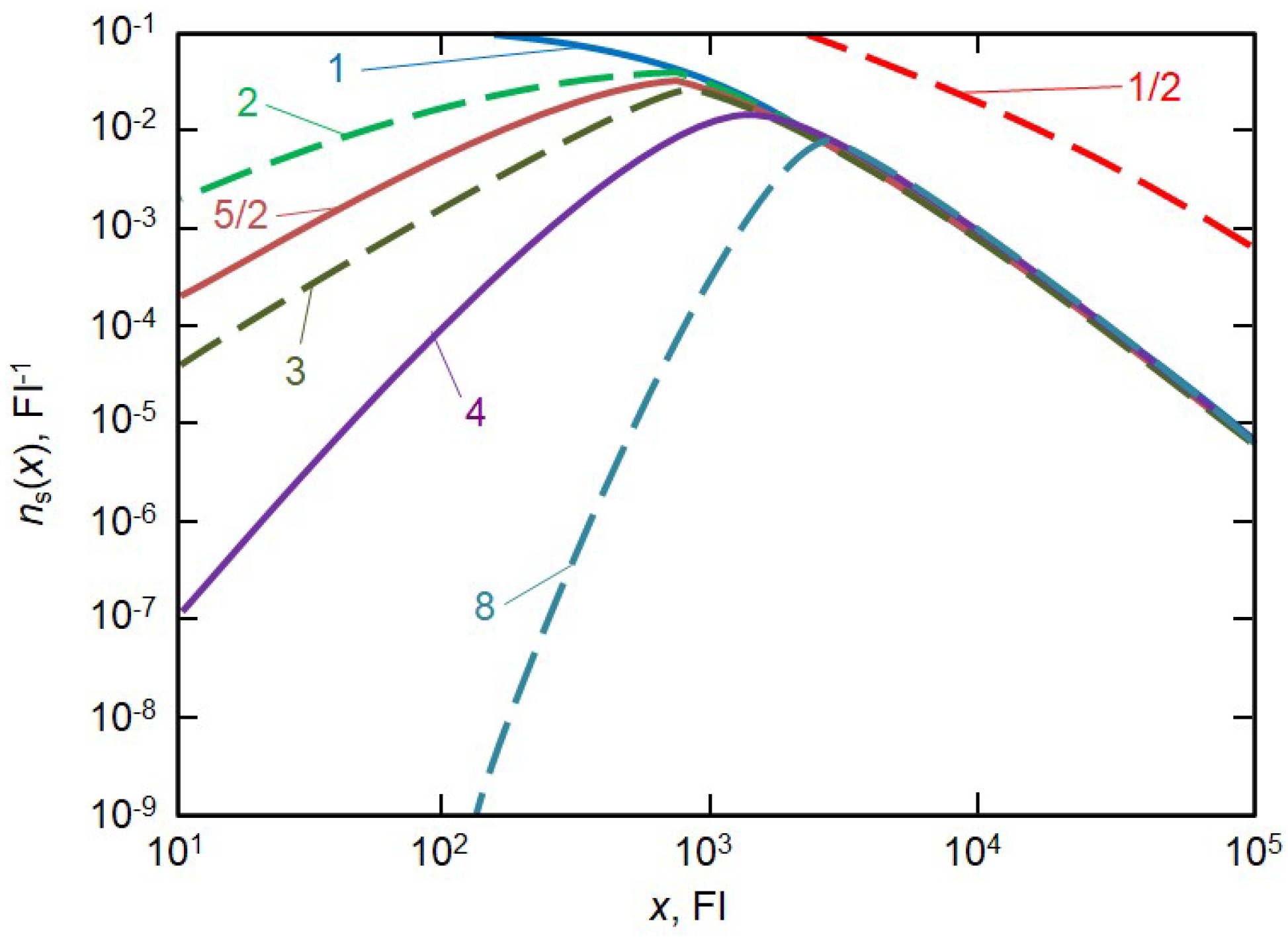
3.1. Integer Values of the Parameter ν

The simplest case for an exponentially decaying source function, which was used in Ref. [24] to describe experimental data of Wang et al. [23] on gold nanoparticle distribution inside endosomes, follows from (6) at ν = 1 and leads to
n ˜ s ( p ) = q ( 1 ) a p + b + ( p + b ) ( p + a ) , a = b 2 J a 2 K x 0 2 .
Now applying the inverse Laplace transform to expression (13) (see 22.95 in [26]), we obtain n s ( x ) at ν = 1
n s ( x ) = J a K x 0 2 exp 1 x 0 J a 2 K x 0 2 x I 0 J x a 2 K x 0 2 + I 1 J x a 2 K x 0 2 ,
where I 0 and I 1 stand for the modified Bessel functions.
The simplest case that takes into account the decay of the source function at x 0 corresponds to ν = 2 . In this case, expression (11) gives
n ˜ s ( p ) = q ( 2 ) a ( p + b ) p + b + ( p + b ) 2 q ( 2 ) / a 2 = q ( 2 ) a ( p + b ) p + a 1 + b 1 2 + ( p + a 1 ) ( p + b 1 ) ,
where
a 1 = b + q ( 2 ) a , b 1 = b q ( 2 ) a .
Now inverting (15) as the convolution of two functions
( p + b ) 1 and p + a 1 + b 1 2 + ( p + a 1 ) ( p + b 1 ) 1
using the tabulated transforms (21.4 and 22.96 in [26]), we arrive at n s ( x ) at ν = 2
n s ( x ) = 2 I * K exp x x 0 0 x ξ 1 I 1 q ( 2 ) a ξ d ξ ,
where q ( 2 ) = 2 I * / K .
A sharper decay of the source function at x 0 occurs at ν = 3 . In this case, expression (11) leads to
n ˜ s ( p ) = a p 1 3 p 1 3 p 1 6 μ 6 = a a p 1 2 μ 2 p 1 3 p 1 2 + μ 2 p 1 μ p 1 2 + μ 2 + p 1 μ = a F ˜ ( p 1 ) f ˜ 3 ( p 1 ) p 1 3 F ˜ ( p 1 ) p 1 2 + f ˜ 3 ( p 1 ) p 1 ,
where
p 1 = p + b , μ = q ( 3 ) a 2 1 / 6 , f ˜ 3 ( p 1 ) = p 1 p 1 2 μ 2 ,
F ˜ ( p 1 ) = f ˜ 1 ( p 1 ) f ˜ 2 ( p 1 ) + f ˜ 1 ( p 1 ) p 1 μ 2 + f ˜ 2 ( p 1 ) p 1 + μ 2 μ 2 4 ,
f ˜ 1 ( p 1 ) = p 1 + μ / 2 2 + 3 μ 2 / 4 p 1 + μ / 2 ,
f ˜ 2 ( p 1 ) = p 1 μ / 2 2 + 3 μ 2 / 4 p 1 μ / 2 .
Now applying the inverse Laplace transform to expression (17) using the tabulated transforms (21.162, 22.165, 22.166 in [26] as well as 2, 3 and 29 in [27]) and their convolutions, we finally obtain n s ( x ) at ν = 3
n s ( x ) = 0 ξ S ( ξ ) 2 π x 3 / 2 exp ξ 2 4 x x x 0 d ξ ,
where
S ( x ) = a 0 x R 0 ( ξ ) R 1 ( x ξ ) d ξ R 0 ( x ) + R 1 ( x ) , R 1 ( x ) = μ 0 x I 1 ( μ ξ ) ξ d ξ ,
R 2 ( x ) = 0 x P ( ξ ) ( x ξ ) d ξ , R 3 ( x ) = 3 μ 2 0 x J 1 3 μ 2 ξ exp μ ξ 2 + exp μ ξ 2 d ξ ξ ,
R 4 ( x ) = 3 μ 2 4 0 x ( x ξ ) J 1 3 μ 2 ξ exp μ ξ 2 exp μ ξ 2 d ξ ξ , R 5 ( x ) = μ 2 x 4 ,
R 0 ( x ) = R 2 ( x ) + R 3 ( x ) + R 4 ( x ) R 5 ( x ) ,
P ( x ) = 3 μ 2 4 0 x J 1 3 μ 2 ξ J 1 3 μ 2 ( x ξ ) exp μ ξ x 2 d ξ x ξ ,
where J 1 is the Bessel function of the first kind.
The next fairly simple case to analyse is a particle source with ν = 4 . In this case, we have from expression (11)
n ˜ s ( p ) = a ( p + b ) 2 ( p + b ) 2 ( p + b ) 4 σ 4 = a σ 2 ( p + b ) 2 a ( p + b ) 2 σ 2 ( p + b ) 2 ( p + b ) 2 + σ 2 ( p + b ) + p + b ( p + b ) 2 σ 2 .
Applying the tabulated inverse Laplace transforms to expression (19) (22.165 and 22.166 from [26] as well as 3, 32, 37 and 48 from [27]), we arrive at the distribution function n s ( x ) at ν = 4
n s ( x ) = a σ 2 x exp x x 0 a σ 0 x exp ξ x 0 J 1 ( σ ξ ) + I 1 ( σ ξ ) Φ ( x ξ ) d ξ ξ ,
where
Φ ( x ) = exp x x 0 cos ( σ x ) + σ 0 x cos σ x 2 ξ 2 I 1 ( σ ξ ) d ξ , σ = q ( 4 ) a 2 1 / 4 .
The method of inverting the stationary image of the distribution function (11) can be applied to other integer values of ν by analogy with the one discussed above. Below we consider just one case at ν = 8 , which is necessary to describe the experimental data [10] on endosomal network dynamics. This particular case corresponds to the source function (6) tending more sharply towards zero at x 0 .
So, expression (11) enables us to obtain the following expression at ν = 8 :
n ˜ s ( p ) = a p 0 4 p 0 4 p 0 8 u 8 = a a p 0 4 p 0 2 u 2 p 0 2 + u 2 p 0 2 + u 2 2 p 0 u × p 0 2 + u 2 + 2 p 0 u = a + a p 0 4 h ˜ 1 ( p 0 ) p 0 h ˜ 2 ( p 0 ) + p 0 h ˜ 3 ( p 0 ) + p 0 u 2 × h ˜ 4 ( p 0 ) + p 0 + u 2 = a i = 1 14 A ˜ i ( p 0 ) ,
where
u = q ( 8 ) a 2 1 / 8 , p 0 = p + b , h ˜ 1 ( p 0 ) = p 0 p 0 2 u 2 , h ˜ 2 ( p 0 ) = p 0 2 + u 2 p 0 ,
h ˜ 3 ( p 0 ) = p 0 u 2 2 + u 2 2 p 0 u 2 ,
h ˜ 4 ( p 0 ) = p 0 + u 2 2 + u 2 2 p 0 + u 2 .
Now applying the inverse Laplace transform to the last expression (21) using the tabulated formulas 21.162, 22.165 and 22.166 in [26], 2 and 3 in [27] as well as their convolutions, we come to n s ( x ) at ν = 8 (additional formulas are given in Appendix A)
n s ( x ) = a i = 1 14 A i ( x ) .
Figure 1 shows a good agreement of the analytical solution (22) with experimental data of Foret et al. [10] on the distribution of low-density lipoprotein (LDL) in the entire network of Rab5-positive endosomes. We should note that in Ref. [10] the variable x stands for the LDL fluorescence intensity, and n represents the density of endosomes per cell such that n ( x ) Δ x is the number of Rab5-positive endosomes per cell for which the LDL fluorescence intensity (FI) is in the interval between x and x + Δ x (for more details, see Ref. [10]). It can be seen from Figure 1 that the LDL concentration is an increasing function of cargo influx J. The latter is directly proportional to the appearance rate of new endosomes carrying the cargo of size x.

3.2. Half-Integer Values of the Parameter ν

Here we consider only two cases with half-integer values of the parameter ν , corresponding to increasing and decreasing source functions (6) at x 0 .
So, dealing with ν = 1 / 2 , we derive from (11)
n ˜ s ( p ) = a p 1 p 1 m 2 p 1 ,
where p 1 = p + b and m = q ( 1 / 2 ) / a . Now using the inverse Laplace transforms 22.158 in Ref. [26] as well as 3, 29 and 134 in Ref. [27], we arrive at n s ( x ) at ν = 1 / 2
n s ( x ) = 1 2 π x 3 / 2 0 ξ exp x x 0 ξ 2 4 x G ( ξ ) d ξ ,
where
G ( x ) = a π 0 x exp m 2 ξ / 2 sinh m 2 ξ / 2 ξ x ξ d ξ .
When deriving expression (24), we also used the following formulas for the Bessel functions
I α ( x ) = i α J α ( i x ) , I 1 / 2 ( x ) = 2 π x sinh x ,
where i is the imaginary unit.
The next function we study here corresponds to ν = 5 / 2 . In this case, we have from (11)
n ˜ s ( p ) = a p 1 5 / 2 p 1 5 χ 5 p 1 5 / 2 = a a p 1 χ p 1 5 / 2 g ˜ 1 ( p 1 ) + p 1 + α 1 χ 2 g ˜ 2 ( p 1 ) + p 1 + β 1 χ 2 ,
where
χ = q ( 5 / 2 ) a 2 1 / 5 , α 1 = 1 5 2 , β 1 = 1 + 5 2 ,
g ˜ 1 ( p 1 ) = p 1 + α 1 χ 2 2 + s 1 2 p 1 + α 1 χ 2 , s 1 = χ 1 α 1 2 / 4 ,
g ˜ 2 ( p 1 ) = p 1 + β 1 χ 2 2 + s 2 2 p 1 + β 1 χ 2 , s 2 = χ 1 β 1 2 / 4 .
Applying the inverse Laplace transform to expression (25) and taking tabulated formulas (22.30, 22.165 in Ref. [26] and 134, 147 in Ref. [27]) into account, we obtain n s ( x ) at ν = 5 / 2
n s ( x ) = 1 2 π x 3 / 2 0 ξ exp x x 0 ξ 2 4 x W ( ξ ) d ξ ,
where W ( ξ ) is given in Appendix B.

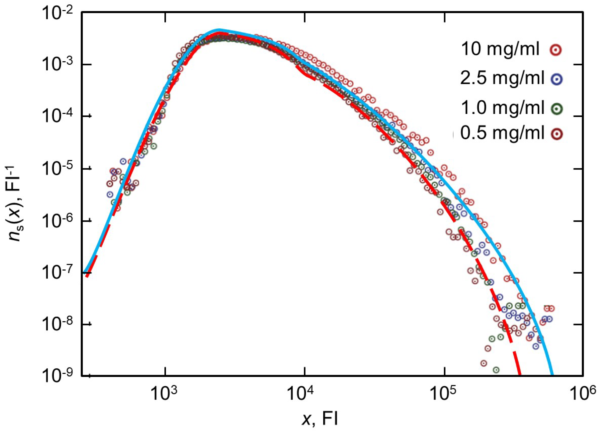
3.3. Source Term with Sub-Linear Prefactor and Exponential Decay

Let us consider here a special case of source term with a sub-linear prefactor whose rate is given by
I ( x ) = I * sin ( ω x ) exp x x 0 ,
where ω is constant. Formula (27) describes the situation when the prefactor grows slowly in a sub-linear manner. We have to choose the parameter ω to ensure the slow growth of the prefactor and its positive value for the relevant values of variable x.
Applying the direct Laplace transform to (27) (Formula (47) in Ref. [27]) and substituting the result into expression (10), we come to
n ˜ s ( p ) = a p 2 p 2 L 2 p 2 , p 2 = ( p + x 0 1 ) 2 + ω 2 , L = 2 I * ω a 2 K .
Applying the inverse Laplace transform to (28) with allowance for the tabulated formulas (22.165 in [26] and 32 in [27]), we arrive at n s ( x ) for the source term with a sub-linear prefactor
n s ( x ) = exp x x 0 R ( x ) ω 0 x R x 2 ξ 2 J 1 ( ω ξ ) d ξ ,
where J 1 is the Bessel function of the first kind and
R ( x ) = a L 0 x J 1 ( L ξ ) ξ d ξ .
A short summary of exact steady-state solutions to Equation (7) is given in Table 1. Based on the data listed in this table, we compare the steady-state distribution functions n s ( x ) (the third column of Table 1) in Figure 2. As is easily seen, the steepness of the curves for small x grows as the parameter ν increases.

4. Unsteady-State Smoluchowski’s Coagulation Equation

4.1. Analytical Solution to the Coagulation Equation without Injection

First, we note that it is possible to obtain an exact solution for the total number of particles of all sizes λ ( τ ) , which is defined by expression (4). To do this, we integrate Equation (3) over the variable x from zero to infinity and obtain
d λ d τ = 1 2 λ 2 + 2 κ λ 2 B , B = 1 K 0 I ( x ) d x .
Its solutions read as
λ ( τ ) = a κ + C ( a + κ ) exp τ 1 C exp τ , C = λ ( 0 ) + κ a λ ( 0 ) + κ + a .
Expressions (30) and (31) represent an exact solution for the total number of particles of all sizes λ ( τ ) in the case of arbitrary source function I ( x ) .
Let us obtain the unsteady solution to (3) for large values of x. In this case, it follows from experimental data of Ref. [10] that the source term is negligible. For example, considering x 10 4 , we estimate the source term I ( x ) / K 10 4 and κ n 10 2 . In this case, (3) becomes
n τ = 1 2 0 x n ( x , τ ) n ( x x , τ ) d x n ( x , τ ) λ ( τ ) κ n ( x , τ ) .
Let us seek for an exact solution to Equation (32) in the form of
n ( x , τ ) = n ( 0 , τ ) exp β ( τ ) x ,
where n ( 0 , τ ) and β ( τ ) are found below. Substituting (33) into (32) and equating the terms with x 0 and x 1 , we obtain two equations
d n ( 0 , τ ) d τ = λ ( τ ) + κ n ( 0 , τ ) , d β d τ = n ( 0 , τ ) 2 .
Their exact solutions are given by
n ( 0 , τ ) = n ( 0 , 0 ) exp κ τ 0 τ λ ( τ 1 ) d τ 1 , β ( τ ) = β ( 0 ) 1 2 0 τ n ( 0 , τ 1 ) d τ 1 .
Here the constants n ( 0 , 0 ) and β ( 0 ) should be chosen by comparing the initial distribution function
n ( x , 0 ) = n ( 0 , 0 ) exp β ( 0 ) x
with experimental data.
An important point of an exact analytical solution (33) to a non-stationary coagulation equation is the exponential initial distribution (36). This can occur if the distribution function relaxes from some initial steady-state exponential distribution. For example, if some distribution is established due to the source contribution I ( x ) , and then the source is switched off, then this distribution will decrease as time increases. This case is described by an exponentially decreasing analytical solution (33).

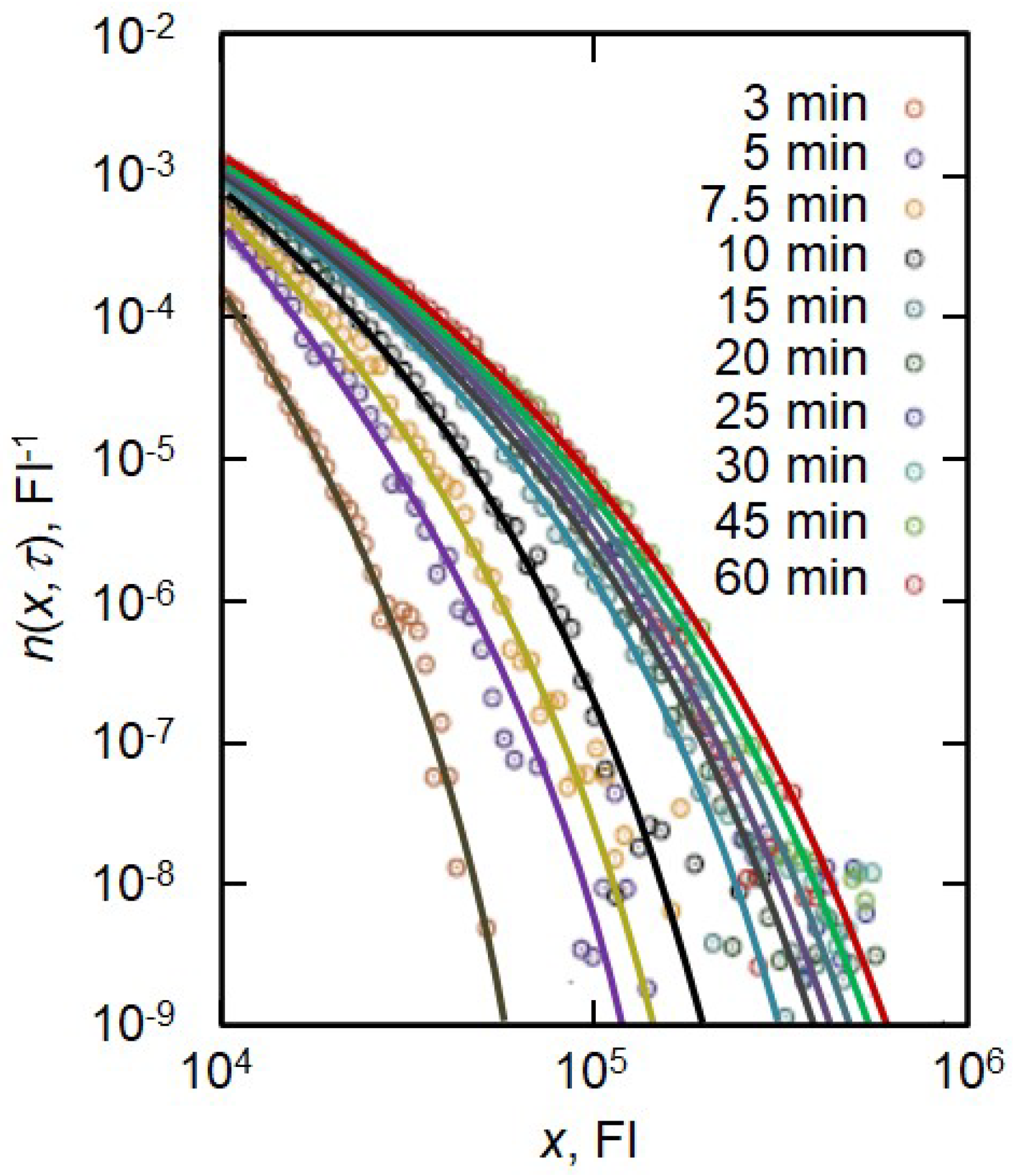
4.2. Approximate Solution to the Unsteady Coagulation Equation with Injection

To compare the theory with experimental data given by Foret et al. [10], we stitch together the initial distribution function n 0 ( x ) (known from experiments) and the steady-state distribution function n s ( x ) at ν = 8 (expression (22)), which is being set at long times. Using the thoughts of Refs. [24,28], we have
n ( x , τ ) = b 0 ( x , τ ) n 0 ( x ) + b s ( x , τ ) n s ( x ) b 0 ( x , τ ) + b s ( x , τ ) .
Here the stitching functions b 0 ( x , τ ) and b s ( x , τ ) should satisfy the following conditions
b 0 ( x , τ ) 0 , τ τ 0 ; b s ( x , τ ) 0 , τ τ 0 ,
where τ 0 is a characteristic time corresponding to the initial distribution n 0 ( x ) . If this is really the case, the unsteady-state distribution function n ( x , τ ) tends to the initial distribution n 0 ( x ) at initial times τ τ 0 , and it approaches the steady-state solution n s ( x ) at large times τ τ 0 . Note that the stitching functions should be chosen by comparing the theory with experiments. So, choosing these functions as
b 0 ( x , τ ) = x 3 / 2 b 0 ( τ τ 0 ) , b s ( x , τ ) = b s ( τ τ 0 ) x 3 / 2 ,
we compare expression (37) with experimental data in Figure 3. As is easily seen, the distribution function n ( x , τ ) grows with time due to the influence of mass influx I ( x ) and always lies between n 0 ( x ) and n s ( x ) .

5. Summary and Conclusions

Let us summarize the main results of our paper. First, we have found an exact stationary solution to Smoluchowski’s coagulation equation with injection in the case of different exponentially decaying source functions. These functions contain a power law factor that substantially changes the steady-state distribution function at small particle volumes x . We have also obtained the exact stationary solution to the coagulation equation with sub-linear exponentially decaying source term. Our steady-state analytical solutions are summarized in Table 1. In addition, we have obtained an analytical solution to the non-stationary integro-differential Smoluchowski’s coagulation equation with injection for large values of particle volumes x when the source term is negligible. This solution is given by expression (33). An approximate analytical solution to the unsteady-state coagulation equation with injection has been constructed using the stitching functions technique. This unsteady-state solution is given by expression (37). Let us especially underline that this distribution depends on stitching functions that enable us to fit its behaviour between the initial and final (steady-state) distributions. Both the steady- and unsteady-state distributions are compared with experimental data for the distributions of endocytosed low-density lipoproteins. An important assumption of our analytical studies is that the collision frequency function (coagulation kernel) K ( x , x ) is taken as a constant. This has allowed us to formulate a relatively simple integro-differential model and solve it using the aforementioned mathematical techniques. Note that the collision frequency function describes different coagulation mechanisms (e.g., Brownian coagulation, shear coagulation, coagulation of particles falling under gravity, mixed coagulation mechanisms [1,2,29,30]). To take such different coagulation mechanisms into account, we can use an approximate method involving the averaging of coagulation kernels over all possible combinations of particle volumes in the steady-state case (see, among others, [22]). This approximate technique will allow to take into account different coagulation mechanisms.
As a special note, the coagulation theory under consideration can be applied to describe the final stage of phase transformations in various metastable and non-equilibrium systems (simultaneous occurrence of Ostwald ripening, coagulation and disintegration of aggregates). These processes, for example, include the growth of inorganic and organic single crystals in metastable and nonequilibrium two-phase regions as well as the production of a cellular glass–ceramic [15,16,17,18,19,31,32,33,34].

Author Contributions

Conceptualization, E.V.M. and S.P.F.; methodology, E.V.M. and D.V.A.; software, E.V.M.; validation, E.V.M. and D.V.A.; formal analysis, E.V.M. and D.V.A.; investigation, S.P.F. and E.V.M.; resources, E.V.M., D.V.A. and S.P.F.; writing—original draft preparation, D.V.A. and E.V.M.; writing—review and editing, E.V.M., D.V.A. and S.P.F.; visualization, E.V.M.; supervision, D.V.A. and S.P.F.; project administration, E.V.M., D.V.A. and S.P.F.; funding acquisition, E.V.M., D.V.A. and S.P.F. All authors have read and agreed to the published version of the manuscript.

Funding

The research funding from the Ministry of Science and High Education of the Russian Federation (Ural Federal University Program of Development within the Priority-2030 Program) is gratefully acknowledged.

Institutional Review Board Statement

Not applicable.

Data Availability Statement

Data is contained within the article.

Conflicts of Interest

The authors declare no conflict of interest.

Appendix A

Here we present the functions entering in expressions (21) and (22) at ν = 8 :
h 1 ( x ) = u I 1 ( u x ) x exp x x 0 , h 3 ( x ) = u 2 x J 1 u x 2 exp u x 2 x x 0 , h 2 ( x ) = u J 1 ( u x ) x exp x x 0 , h 4 ( x ) = u 2 x J 1 u x 2 exp u x 2 x x 0 ,
A 1 ( x ) = 1 Γ ( 4 ) 0 x ξ 3 exp ξ x 0 h 1234 ( x ξ ) d ξ , A 2 ( x ) = u 2 Γ ( 4 ) 0 x ξ 3 exp ξ x 0 × h A 2 ( x ξ ) d ξ , A 3 ( x ) = 1 Γ ( 3 ) 0 x ξ 2 exp ξ x 0 h A 3 ( x ξ ) d ξ , A 4 ( x ) = u 2 2 Γ ( 4 ) 0 x ξ 3 exp ξ x 0 h 12 ( x ξ ) d ξ , A 5 ( x ) = 1 Γ ( 3 ) 0 x ξ 2 exp ξ x 0 h A 5 ( x ξ ) d ξ , A 6 ( x ) = u 2 Γ ( 3 ) 0 x ξ 2 exp ξ x 0 × h 13 ( x ξ ) h 14 ( x ξ ) h 23 ( x ξ ) + h 24 ( x ξ ) d ξ , A 7 ( x ) = 1 Γ ( 2 ) 0 x ξ exp ξ x 0 h 13 ( x ξ ) + h 14 ( x ξ ) h 23 ( x ξ ) h 24 ( x ξ ) d ξ , A 8 ( x ) = u 2 2 Γ ( 3 ) 0 x ξ 2 exp ξ x 0 h 1 ( x ξ ) h 2 ( x ξ ) d ξ , A 9 ( x ) = 1 Γ ( 2 ) 0 x ξ exp ξ x 0 h 34 ( x ξ ) d ξ , A 10 ( x ) = u 2 Γ ( 2 ) 0 x ξ exp ξ x 0 × h 3 ( x ξ ) h 4 ( x ξ ) d ξ , A 11 ( x ) = 0 x exp ξ x 0 h 3 ( x ξ ) + h 4 ( x ξ ) d ξ , A 12 ( x ) = u 2 x 2 exp x x 0 , A 13 ( x ) = 0 x ξ exp ξ x 0 h 12 ( x ξ ) d ξ , A 14 ( x ) = 0 x exp ξ x 0 h 1 ( x ξ ) h 2 ( x ξ ) d ξ ,
where
h 1234 ( x ) = 0 x h 12 ( ξ ) h 34 ( x ξ ) d ξ , h 12 ( x ) = 0 x h 1 ( ξ ) h 2 ( x ξ ) d ξ , h 34 ( x ) = 0 x h 3 ( ξ ) h 4 ( x ξ ) d ξ , h A 2 ( x ) = 0 x h 12 ( ξ ) h 3 ( x ξ ) h 4 ( x ξ ) d ξ , h A 3 ( x ) = 0 x h 12 ( ξ ) h 3 ( x ξ ) + h 4 ( x ξ ) d ξ , h A 5 ( x ) = 0 x h 34 ( ξ ) h 1 ( x ξ ) h 2 ( x ξ ) d ξ , h 13 ( x ) = 0 x h 1 ( ξ ) h 3 ( x ξ ) d ξ , h 14 ( x ) = 0 x h 1 ( ξ ) h 4 ( x ξ ) d ξ , h 23 ( x ) = 0 x h 2 ( ξ ) h 3 ( x ξ ) d ξ , h 24 ( x ) = 0 x h 2 ( ξ ) h 4 ( x ξ ) d ξ .

Appendix B

Here we present the functions entering in expression (26) at ν = 5 / 2 :
W ( x ) = i = 1 3 W i ( x ) , W 1 ( x ) = a 2 π 0 x exp χ ξ 1 ξ 3 / 2 x ξ d ξ ,
W 2 ( x ) = a α 1 β 1 χ 2 4 B 2 ( x ) x + a χ ( α 1 + β 1 ) 2 B 3 ( x ) 1 + a 0 x B 2 ( ξ ) ξ H ( x ξ ) d ξ ,
W 3 ( x ) = a 0 x B 3 ( ξ ) 1 g 1 ( x ξ ) + g 2 ( x ξ ) d ξ ,
H ( x ) = B 1 ( x ) + χ 2 ( β 1 g 1 ( x ) + α 1 g 2 ( x ) ) , B 1 ( x ) = 0 x g 1 ( ξ ) g 2 ( x ξ ) d ξ ,
B 2 ( x ) = 1 2 π Γ ( 5 / 2 ) 0 x exp ( χ ξ ) 1 ξ 3 / 2 ( x ξ ) 3 / 2 d ξ ,
B 3 ( x ) = 1 2 π Γ ( 3 / 2 ) 0 x exp ( χ ξ ) 1 ξ 3 / 2 ( x ξ ) 1 / 2 d ξ ,
g 1 ( x ) = s 1 x J 1 ( s 1 x ) exp α 1 χ 2 x , g 2 ( x ) = s 2 x J 1 ( s 2 x ) exp β 1 χ 2 x .

References

  1. Friedlander, S.K. Smoke, Dust, and Haze: Fundamentals of Aerosol Dynamics; Oxford University Press: Oxford, UK, 2000. [Google Scholar]
  2. Williams, M.M.R.; Loyalka, S.K. Aerosol Science: Theory and Practice; Pergamon Press: Oxford, UK, 1991. [Google Scholar]
  3. Hayakawa, H. Irreversible kinetic coagulations in the presence of a source. J. Phys. A Math. Gen. 1987, 20, 801–805. [Google Scholar] [CrossRef]
  4. Takayasu, H. Steady-state distribution of generalized aggregation system with injection. Phys. Rev. Lett. 1989, 63, 2563–2565. [Google Scholar] [CrossRef] [PubMed]
  5. Cueille, S.; Sire, C. Droplet nucleation and Smoluchowski’s equation with growth and injection of particles. Phys. Rev. E 1998, 57, 881–900. [Google Scholar] [CrossRef]
  6. Alexandrov, D.V. Kinetics of particle coarsening with allowance for Ostwald ripening and coagulation. J. Phys. Condens. Matter 2016, 28, 035102. [Google Scholar] [CrossRef] [PubMed]
  7. Alexandrov, D.V.; Ivanov, A.A.; Alexandrova, I.V. Unsteady-state particle-size distributions at the coagulation stage of phase transformations. Eur. Phys. J. Spec. Top. 2019, 228, 161–167. [Google Scholar] [CrossRef]
  8. Castro, M.; Lythe, G.; Smit, J.; Molina-París, C. Fusion and fission events regulate endosome maturation and viral escape. Sci. Rep. 2021, 11, 7845. [Google Scholar] [CrossRef]
  9. Fedotov, S.; Alexandrov, D.; Starodumov, I.; Korabel, N. Stochastic model of virus-endosome fusion and endosomal escape of pH-responsive nanoparticles. Mathematics 2022, 10, 375. [Google Scholar] [CrossRef]
  10. Foret, L.; Dawson, J.E.; Villaseñor, R.; Collinet, C.; Deutsch, A.; Brusch, L.; Zerial, M.; Kalaidzidis, Y.; Jülicher, F. A general theoretical framework to infer endosomal network dynamics from quantitative image analysis. Curr. Biol. 2012, 22, 1381–1390. [Google Scholar] [CrossRef]
  11. Smoluchowski, M. Drei Vortrage uber Diffusion, Brownsche Bewegung und Koagulation von Kolloidteilchen. Z. Phys. 1916, 17, 557–585. [Google Scholar]
  12. Smoluchowski, M. Versuch einer mathematischen theorie der koagulationskinetik kolloider losungen. Z. Phys. Chem. 1917, 92, 129–168. [Google Scholar] [CrossRef]
  13. Simons, S. On steady-state solutions of the coagulation equation. J. Phys. A Math. Gen. 1996, 29, 1139–1140. [Google Scholar] [CrossRef]
  14. Alexandrov, D.V. The steady-state solutions of coagulation equations. Int. J. Heat Mass Trans. 2018, 121, 884–886. [Google Scholar] [CrossRef]
  15. Herlach, D.; Galenko, P.; Holland-Moritz, D. Metastable Solids from Undercooled Melts; Elsevier: Amsterdam, The Netherlands, 2007. [Google Scholar]
  16. Barlow, D.A. Theory of the intermediate stage of crystal growth with applications to protein crystallization. J. Cryst. Growth 2009, 311, 2480–2483. [Google Scholar] [CrossRef]
  17. Barlow, D.A. Theory of the intermediate stage of crystal growth with applications to insulin crystallization. J. Cryst. Growth 2017, 470, 8–14. [Google Scholar] [CrossRef]
  18. Alexandrova, I.V.; Alexandrov, D.V.; Makoveeva, E.V. Ostwald ripening in the presence of simultaneous occurrence of various mass transfer mechanisms: An extension of the Lifshitz–Slyozov theory. Philos. Trans. R. Soc. A 2021, 379, 20200308. [Google Scholar] [CrossRef] [PubMed]
  19. Ramírez Zamora, R.M.; Espejel Ayala, F.; Solís López, M.; González Barceló, O.; Gómez, R.W.; Pérez Mazariego, J.L.; Navarro-González, R.; Schouwenaars, R. Optimisation and analysis of the synthesis of a cellular glass-ceramic produced from water purification sludge and clays. Appl. Clay Sci. 2016, 123, 232–238. [Google Scholar] [CrossRef]
  20. Buyevich, Y.A.; Natalukha, I. Unsteady processes of combined polymerization and crystallization in continuous apparatuses. Chem. Eng. Sci. 1994, 49, 3241–3247. [Google Scholar] [CrossRef]
  21. Alexandrov, D.V.; Ivanov, A.A.; Nizovtseva, I.G.; Lippmann, S.; Alexandrova, I.V.; Makoveeva, E.V. Evolution of a polydisperse ensemble of spherical particles in a metastable medium with allowance for heat and mass exchange with the environment. Crystals 2022, 12, 949. [Google Scholar] [CrossRef]
  22. Schumann, T.E.W. Theoretical aspects of the size distribution of fog particles. Q. J. R. Meteorol. Soc. 1940, 66, 195–208. [Google Scholar] [CrossRef]
  23. Wang, S.H.; Lee, C.W.; Tseng, F.G.; Liang, K.K.; Wei, P.K. Evolution of gold nanoparticle clusters in living cells studied by sectional dark-field optical microscopy and chromatic analysis. J. Biophotonics 2016, 9, 738–749. [Google Scholar] [CrossRef]
  24. Alexandrov, D.V.; Korabel, N.; Currell, F.; Fedotov, S. Dynamics of intracellular clusters of nanoparticles. Cancer Nanotechnol. 2022, 13, 15. [Google Scholar] [CrossRef]
  25. Alexandrova, I.V.; Alexandrov, D.V. A complete analytical solution of unsteady coagulation equations and transition between the intermediate and concluding stages of a phase transformation. Eur. Phys. J. Spec. Top. 2022, 231, 1115–1121. [Google Scholar] [CrossRef]
  26. Ditkin, V.A.; Prudnikov, A.P. Integral Transforms and Operational Calculus; Pergamon Press: Oxford, UK, 1965. [Google Scholar]
  27. von Doetsch, G. Anleitung zum Praktischen Gebrauch der Laplace-Transformation und der Z-Transformation; R. Oldenbourg: München, Germany, 1967. [Google Scholar]
  28. Alexandrov, D.V.; Galenko, P.K. The shape of dendritic tips. Philos. Trans. R. Soc. A 2020, 378, 20190243. [Google Scholar] [CrossRef]
  29. Hunt, J.R. Self-similar particle-size distributions during coagulation: Theory and experimental verification. J. Fluid Mech. 1982, 122, 169–185. [Google Scholar] [CrossRef]
  30. Alexandrov, D.V.; Ivanov, A.A.; Alexandrova, I.V. The influence of Brownian coagulation on the particle-size distribution function in supercooled melts and supersaturated solutions. J. Phys. A Math. Theor. 2019, 52, 015101. [Google Scholar] [CrossRef]
  31. Martin, S.; Kauffman, P. The evolution of under-ice melt ponds, or double diffusion at the freezing point. J. Fluid Mech. 1974, 64, 507–527. [Google Scholar] [CrossRef]
  32. Huppert, H.E. The fluid mechanics of solidification. J. Fluid Mech. 1990, 212, 209–240. [Google Scholar] [CrossRef]
  33. Alexandrov, D.V.; Aseev, D.L. One-dimensional solidification of an alloy with a mushy zone: Thermodiffusion and temperature-dependent diffusivity. J. Fluid Mech. 2005, 527, 57–66. [Google Scholar] [CrossRef]
  34. Peppin, S.S.L.; Huppert, H.E.; Worster, M.G. Steady-state solidification of aqueous ammonium chloride. J. Fluid Mech. 2008, 599, 465–476. [Google Scholar] [CrossRef]
Figure 1. Theory (expression (22)) is compared with experimental distribution (Figure 3E in Ref. [10]) after 45 min internalization of low-density lipoprotein (LDL) for four different LDL concentrations: γ = 0.0015 s 1 ; K = 0.00016 s 1 , x 0 = 450 FI; J = 546 FI s 1 (blue solid line) and J = 300 FI s 1 (red dashed line).
Crystals 12 01159 g001
Figure 2. The steady-state density distribution functions n s ( x ) at different I ( x ) and ν (numbers at the curves) accordingly to Table 1. System parameters correspond to Figure 1 and J = 546 FI s 1 .
Crystals 12 01159 g002
Figure 3. The unsteady-state density distribution functions n ( x , τ ) at different times accordingly to an analytical solution (37) (lines) and experimental data [10] (symbols). System parameters correspond to Figure 1 and J = 546 FI s 1 , b 0 = b s = 5 × 10 5 . The initial distribution function n 0 ( x ) was chosen at τ 0 = 3 min.
Crystals 12 01159 g003
Table 1. A short summary of exact steady-state solutions.
ν I ( x ) n s ( x ) I ˜ ( 0 ) I * q ( ν )
1 / 2 I * x 1 / 2 exp x x 0 Equation (24) 2 J x 0 2 J π x 0 3 / 2 4 J K x 0 3 / 2
1 I * exp x x 0 Equation (14) J x 0 J x 0 2 2 J K x 0 2
2 I * x exp x x 0 Equation (16) J 2 x 0 J 2 x 0 3 J K x 0 3
5 / 2 I * x 3 / 2 exp x x 0 Equation (26) 2 J 5 x 0 8 J 15 π x 0 7 / 2 4 J 5 K x 0 7 / 2
3 I * x 2 exp x x 0 Equation (18) J 3 x 0 J 6 x 0 4 2 J 3 K x 0 4
4 I * x 3 exp x x 0 Equation (20) J 4 x 0 J 24 x 0 5 J 2 K x 0 5
8 I * x 7 exp x x 0 Equation (22) J 8 x 0 J 40 , 320 x 0 9 J 4 K x 0 9
- I * sin ω x exp x x 0 Equation (29) ( ω 2 x 0 2 + 1 ) J 2 x 0 ( ω 2 x 0 2 + 1 ) 2 J 2 ω x 0 3 -
Publisher’s Note: MDPI stays neutral with regard to jurisdictional claims in published maps and institutional affiliations.

