Article

Development of the Concurrent Multiscale Discrete-Continuum Model and Its Application in Plasticity Size Effect

EPSRC Future Metrology Hub, Centre for Precision Technologies, University of Huddersfield, Huddersfield HD1 3DH, UK
*
Author to whom correspondence should be addressed.
Crystals 2022, 12(3), 329; https://doi.org/10.3390/cryst12030329
Submission received: 28 January 2022 / Revised: 16 February 2022 / Accepted: 25 February 2022 / Published: 26 February 2022
(This article belongs to the Special Issue Applications of Crystal Plasticity in Forming Technologies)

Abstract

:
A concurrent multiscale model coupling discrete dislocation dynamics to the finite element method is developed to investigate the plastic mechanism of materials at micron/submicron length scales. In this model, the plastic strain is computed in discrete dislocation dynamics (DDD) and transferred to the finite element method (FEM) to participate in the constitutive law calculation, while the FEM solves the complex boundary problem for DDD simulation. The implementation of the whole coupling scheme takes advantage of user subroutines in the software ABAQUS. The data structures used for information transferring are introduced in detail. Moreover, a FE mesh-based regularization method is proposed to localize the discrete plastic strain to continuum material points. Uniaxial compression tests of single crystal micropillars are performed to validate the developed model. The results indicate the apparent dependence of yield stress on sample size, and its underlying mechanisms are also analyzed.

1. Introduction

The effect of sample size or shape on material deformation behavior [1,2,3] has received attention for decades. For instance, the sample size of concrete influences its kinetics of external sulfate attack [4]. At the microscale, it has been reported that the deformation mechanism of crystal materials is different from that of bulk materials [5,6,7]. It is recognized that the strength of micro/submicron crystals depends not only on the material itself but also the sample/grain size. Many efforts have been made to study the size effects of crystal materials at the micro/submicron scale in order to improve material performance for high-quality products [8,9,10,11]. The size effect is induced by many physical mechanisms, such as dislocation motion, nucleation, and starvation [12,13]. It remains difficult to capture the full picture of the deformation behavior of crystal material at the micro/nano-scale only by experimental tests. Therefore, it is necessary to employ a suitable simulation method to reveal the underlying deformation mechanisms of crystal materials at the micro/nano-scale.
Computational simulation methodologies have been continuously developed to predict material deformation behaviors. According to the difference in simulation scale, the main simulation methods can be broadly classified into the finite element method (FEM) [14,15], crystal plasticity finite element methods (CPFEMs) [16,17], discrete dislocation dynamics (DDD) [8,18,19], and molecular dynamics (MD) [20]. Based on empirical constitutive equations, the FEM shows a great advantage in dealing with various complex boundary problems at the macroscale. Compared to the classic FEM, CPFEMs consider the material microscopic plastic shear deformation by employing critical parameters that represent the microstructural state of materials beneath the materials’ macroscopic deformation. Typical examples are the slip systems-based phenomenological CPFEMs and the dislocation density-based CPFEM. Moreover, by considering the density of geometrically necessary dislocations (GNDs) in the constitutive equations, it can be used to predict the size effect of crystal materials because GNDs are related to the strain gradient and has been considered in the constitutive equation [21,22,23,24]. However, CPFEMs cannot provide an explicit microstructure evolution during the deformation process, because of the empirical constitutive equation used. To obtain insight into the physical deformation mechanism, a microscale simulation model that considers the intrinsic microstructure characteristics of crystal materials is needed. MD simulation directly depicts the interaction of atoms. In recent decades, it has been widely employed to investigate the mechanical properties of single crystals and nanopolycrystalline materials (e.g., nano-polycrystal silicon [25] and copper [26]) by means of nanoindentation or many other tests [11]. However, MD simulation is only suitable for nanoscale specimens due to the extremely heavy computational load. Indeed, the plastic deformation of crystals results from its dislocation activities. To overcome those limitations, DDD has been proposed by many researchers to capture the size effect and uncover its underlying mechanisms. It omits the direct atomic interactions and takes dislocation as the intrinsic carrier of plastic strain. DDD modeling is often employed together with the FEM to deal with complex boundary conditions. The mostly used coupling schemes are the discrete continuous model (DCM) [27] and superposition method (SPM) [28].
To solve the boundary value problem of a finite crystal, van der Giessen and Needleman [28] first proposed the concept of the SPM. In the SPM, the total stress field in a finite crystal is the sum of two stress fields. One is the analytical stress field due to the existence of dislocations in an infinite unbounded crystal and the other is the complementary elastic stress field calculated by finite element analysis in a finite crystal. The method is able to capture the short-range dislocation stress field accurately and has been improved by incorporating a 3D dislocation mechanism [13,29] and dislocation climb [30]. Nevertheless, the calculation of the analytical stress field between all existing dislocations is time-consuming. In addition, there is no explicit introduction of the plastic strain that arises from dislocation activities. The DCM is another hybrid approach coupling DDD to the FEM. The numerical calculation in the DCM is straightforward and has clear physical sense. The moving dislocation generates plastic strain along its gliding path, and then the plastic strain is localized to the Gaussian integration points of the FEM. By making use of the plastic strain, the equilibrium stress is computed in the FEM module and is used to drive the movement of discrete dislocations.
Since Lemarchand [27] first proposed the DCM in 2001, it has been widely used to study the plastic behavior of materials at micron/submicron length scales, for example, the effect of hard coating [31], low-amplitude cyclic loading [32], temperature [33], and shock loading [34] on the plastic deformation of micropillars. The dislocation mechanisms causing the channel size effects of superalloys [12], incipient plastic instability of nanoindentation [35], and strain bursts of micropillars [10] have been investigated using the DCM. Recently, Cui et al. [31] studied the confined plasticity in coated micropillars using the DCM and found that the operation of a single arm source plays a key role in the plastic deformation of coated pillars. Santos-Güemes et al. [36] studied the interaction mechanism of dislocation and precipitates using a developed multi-scale DCM. The intrinsic hardening mechanism of a nickel-based superalloy and its dependence on the interfacial dislocation network and lattice mismatch were reported [37]. By introducing a dislocation climb model into the DCM, Liu et al. [38] investigated the high-temperature anneal hardening behavior of an Au submicron-pillar.
Most studies are focused on the application of the DCM in plastic mechanisms at micron/submicron scales; however, less attention has been paid to its numerical algorithms for improved computational efficiency. Zbib et al. [39] proposed a simple method of regularizing the plastic strain induced by dislocations to the material points of their localized elements. Liu et al. [40] introduced the Burgers vector density function to apportion the discrete plastic strain to the corresponding material points. Vattré [41] and Cui [42] also discussed the detailed numerical algorithm of localizing the discrete strain to continuum material points in a 3D DCM simulation. In addition, the strain regularization method in a 2D DCM was developed by Huang [30] by considering the interaction of dislocation with its neighboring inter-phase boundaries and other dislocations. However, the computational load remains a challenge in computational simulation. There is always a balance of numerical accuracy and computational efficiency.
In this paper, a concurrent multiscale model coupling DDD to the FEM is developed to investigate the plastic mechanism of materials at micron/submicron length scales. A FE mesh-based regularization method is proposed to improve the computational efficiency. The implementation details of how to apply the DCM principle to couple DDD with FEM calculation modules during the deformation process are introduced. The optimized data structure and the achievement of the simultaneous coupling scheme by subroutines are presented for the first time. The description of the 2D-DCM is provided in Section 2. Section 3 discusses transfer methods of plastic strain and stress among DDD and FEM modules. The user subroutines of Abaqus used in the multiscale framework are described in detail in Section 4. In Section 5, a compression test of a single crystal is performed using the developed method, and it is followed with some main conclusions drawn in Section 6.

2. Description of DCM Coupling Framework

As schematically illustrated in Figure 1, the multiscale framework consists of two modules, i.e., DDD and FEM module. The key point of the 2D-DCM is that the plastic strain calculated by DDD directly participates in the constitutive law of the FEM. The stress tensor at simulation step n, σ n , is expressed as,
σ n = [ C e ] : ε n t ε n 1 p
where ε n 1 p is the plastic strain at the last step by DDD, ε n t is the total strain at simulation step n , and C e is the elastic moduli tensor. The explicit computation of movement, evolution, and interaction between dislocations and other defects (e.g., obstacles, dislocation, and sources) is performed in DDD. In addition, the calculation of the equilibrium stress field in the FEM module and the coupling algorithm of both modules are discussed.

2.1. Two-Dimensional Dislocation Dynamics

For the 2D plane strain problem discussed in this paper, only edge dislocations are considered. The effect of dislocation climb is also negligible compared with that of dislocation glide. The driving force applied on dislocations can be expressed as
f i = n i · σ i · b i ,
where n i is a unit normal to the slip plane, b i is the Burgers vector, and σ i is the stress tensor at the position of dislocation i, which is evaluated in the FEM.
Assuming that the edge dislocations can reach a stable velocity instantly, the glide velocity of dislocation i is
v i = f i B ,
where B is the viscous drag coefficient.
Static point sources are distributed on the slip plane randomly to mimic the operation of Frank–Read sources. A dislocation dipole is generated once the shear stress at the point source exceeds its critical strength, τ n u c , during a time period. The initial distance L n u c between two newly generated dislocations is
L n u c = μ 2 π 1 ν   b τ n u c ,
where μ is the shear modulus and ν is the Poisson ratio of crystal material.
Two dislocations with opposite Burgers vectors annihilate each other when their distance is less than the critical annihilation distance L e , which is taken as 6b [43,44].
The motion of dislocations can be impeded by various obstacles, such as small precipitates and forest dislocation. The point obstacles are modeled in 2D-DDD to consider the effect of the obstacles existing in real crystals [43,45]. If one obstacle lies on the gliding path of a dislocation, the dislocation is pinned by the obstacle when its resolved shear stress is less than the strength of the obstacle. Dislocations can be de-pinned or bypass the obstacle if its shear stress exceeds the obstacle strength.

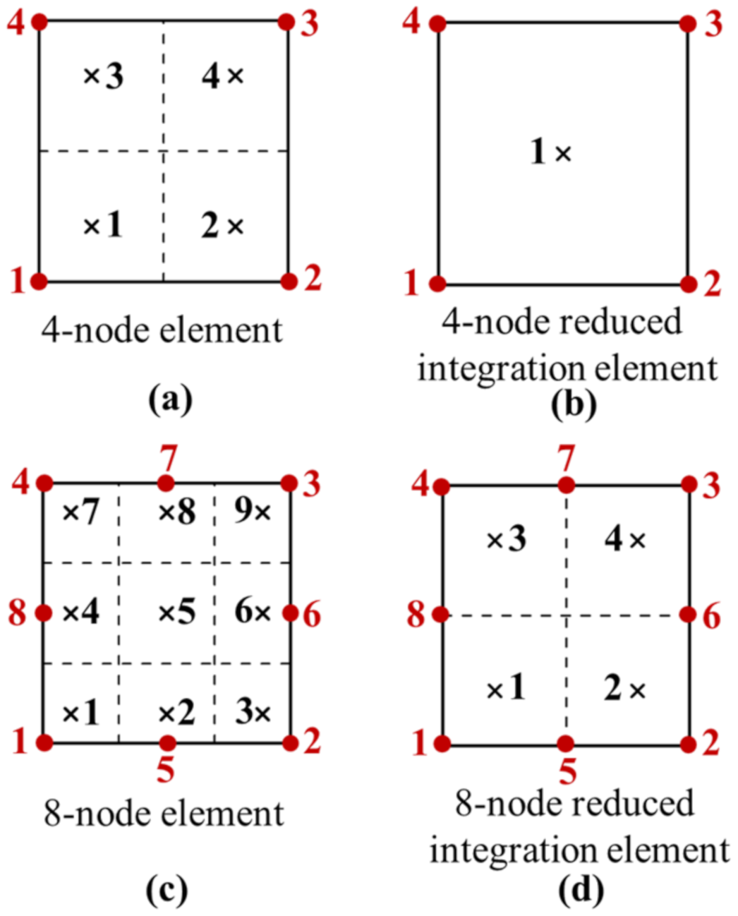
2.2. Calculation in Finite Element Module

The standard FEM is employed to solve the boundary value problem of a finite crystal as follows:
K U = f a + f p ,
f p = V   C e ε p B d V ,
where [K] is stiffness matrix, U is the nodal displacement vector, f a is the applied force vector, f p is the force vector from plastic strain, [B] = grad[N], and [N] is the shape function vector. The DDD module contributes the plastic strain ε p to the unified continuum mechanics framework.

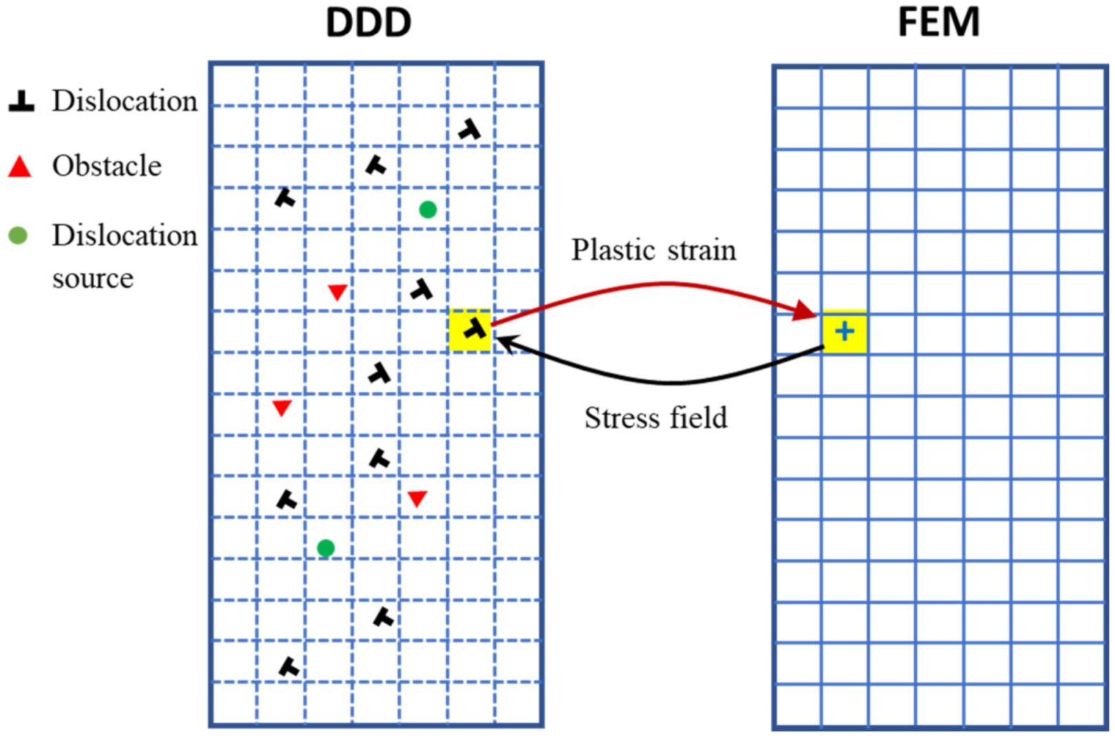
3. Plastic Strain–Stress Transfer in Coupling Scheme

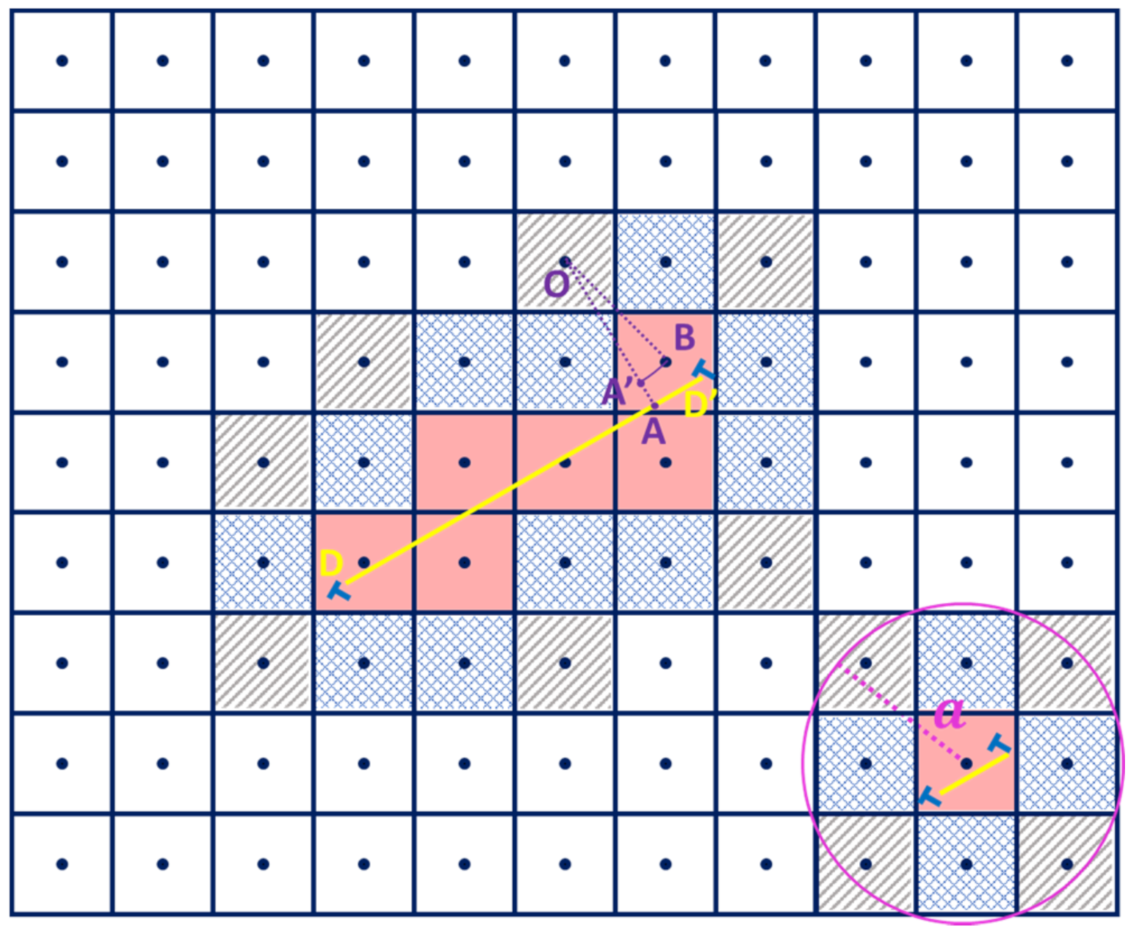
3.1. Plastic Strain and Stress Transfer Scheme

In this computational simulation model, the plastic strain is explicitly calculated in the DDD module and is then transferred to Gaussian integration points of the FEM module for the constitutive calculation. The plastic strain is induced by the glide of dislocation, which can be calculated as:
ε i p = A i 2 V n i b i + b i n i ,
where A i is the swept area of the dislocation i and V is the representative volume.
The plastic strain ε i p obtained from the DDD module should be located at the corresponding integration points as the eigen-strains. Different regularization methods have been proposed to solve this problem. In the early work by Lemarchand [27], it was assumed that a slab with finite thickness h surrounding the glide plane represents the elementary slip events. The elementary volume associated with each Gauss integration point is taken as the representative volume. The plastic strain distributed at each integration point depends on the intersection volume between the slab and elementary volume. Based on the work of Lemarchand [27], Liu [40] proposed a weight function (i.e., the Burgers vector density function) to distribute the total plastic strain to each integration point of finite element. Vattré [41] and Cui [42] also made efforts to improve the regularization method of plastic strain. For the 2D computational model, Huang [30] presented a detailed regularization procedure, which is similar to that of Liu [40]. A local domain along the slip plane of dislocation was defined and half of its width was set as a , which is analogous to the dislocation core spreading radius. The integration points in the local domain would be allocated with plastic strain, and the allocation proportion of each integration point was decided by its distance to the slip plane of dislocation. This regularization method can relieve a high gradient of plastic strain among neighboring elements. However, it causes a heavy computational burden, especially when numerous dislocations exist in the simulation model, due to the distances between each integration point, and the slip plane should be calculated.
An efficient regularization method is proposed in this paper by considering the characteristics of meshes of the FEM model. Elements in the FEM model are divided into elementary domains (i.e., integration point domain), which are associated with each integration point in the elements. As shown in Figure 2, a dislocation glides along its slip plane from D to D’. These elementary domains intersecting with the gliding path are regarded as ‘core domains,’ which are shown as the red domains in Figure 2. If the distance from the integration point of an elementary domain to a core domain is less than the given value a , the elementary domain k is defined as a ‘secondary domain.’ The hatched and meshed areas represent the secondary domains in Figure 2. The parameter a has the same meaning and evaluation as the one used in Huang’s method. The core and secondary domains together compose the domain Ω i . The localized plastic strain of integration point j, ε i j p , in the domain Ω i is given according to a weight function,
ε i j p = ω j j ω j A i 2 V   n i b i + b i n i ,
where ω j is the distribution coefficient for plastic strain caused by dislocation i on integration point j . The value of ω j , which is selected as the Burgers vector spreading function developed by Cai [46], can be calculated as
ω j = 1 r j 2 + a 2 3.5 ,
where r j is the distance between the integration points of the j-th elementary domain and its nearest core domain. For the integration point O shown in Figure 2, the distance is equal to the length of O B , and it replaces the length of O A used by Huang [47]. The simplification of r j makes it easier to obtain the distribution coefficient. Instead of solving the formula for the distance from point to line, it only needs the distance between the integration points of the core and secondary domain. Once the core domains are obtained, the secondary domains around them can be quickly captured according to the numbering order of integration points and elements. Figure 3 shows the numbering order of integration points in different elements. The new method omits the determination of the gliding path equations of each dislocation by replacing the glide path with the core domain. Thus, with the present method, it is computationally efficient to capture the influenced domain, Ω i , of each moving dislocation and calculate the distribution coefficient through directly solving the distance formula of two points.
After FEM calculation, there are two steps to transfer the stress field from the FEM module to the DDD module, i.e., (i) stress extrapolation from integration points to nodes by the inverse shape function, and (ii) stress interpolation from nodes to dislocations by the shape function of the element [41]. In finite element analysis, the numerical integration is carried out at the Gaussian points and the stress value at the integration point is the most accurate. Therefore, in this work, the stress of dislocations is determined by the integration point domain where dislocations reside. The stress tensor of a dislocation is the same as its nearest Gaussian integration point. The division of various elements into integration point domains is illustrated in Figure 3. Each domain contains one integration point and any point in the domain has the shortest distance to the contained integration point compared to other integration points in the parent element. The number of integration points in the parent element is determined by the degree of the integrated polynomial terms in the element’s stiffness matrix and the desired accuracy of results. According to the number of integration points required, their locations in the parent element can be obtained by Table 1.

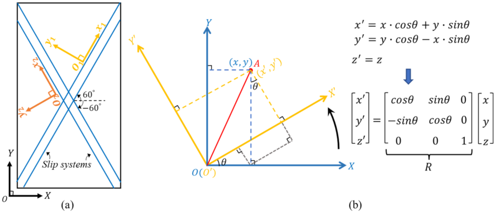
3.2. Coordinate System Conversion Involved in Coupling Scheme

In order to complete the data exchange between DDD and the FEM module, the transformation of the coordinate system should be taken into account.
The calculation in the DDD module, such as glide force, dislocation velocity, and plastic strain, is finished on the local coordinate system whose axes are consistent with the slip direction and normal direction of the slip plane, as shown in Figure 4a. The FEM module is constructed in the sample coordinate system, unlike that of the DDD module. To achieve the coordinate system transformation, the transformation matrix, R , is calculated by representing the vector O A in the two coordinate frames, as illustrated in Figure 4b. Then, the vectors, {g}, and tensors, [M], can be transformed with rules as follows:
g = R g ,
M = R T M R ,
where g and M are the transformed vector and tensor, respectively. Superscript T means matrix transpose.

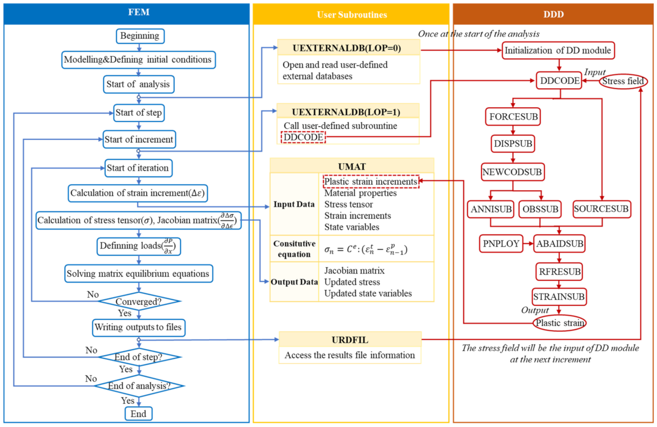
4. Subroutines for ABAQUS

The multiscale framework is built by the secondary development of finite element software ABAQUS. In this section, the implementation details of the DCM model in ABAQUS are introduced.

4.1. User Subroutines in the Multiscale Framework

Abundant user subroutines are provided in ABAQUS, which allow advanced users to customize a variety of ABAQUS capabilities [48]. The general workflow for running the DCM using ABAQUS is illustrated in Figure 5. Three user subroutines are used for the DCM model, including URDFIL for results processing, UEXTERNALDB for external file manipulation, and UMAT for the physics-based constitutive law. The functions of these subroutines in the developed model are discussed below.
A user subroutine called URDFIL is written particularly as a stress relay from the FEM to DDD module. The subroutine performs two functions: it can access the results file for stress tensors of Gaussian integration points, nodes coordinates, elements, and its relative integration point numbers at the end of the increment, and it transfers this new information to the DDD module by writing them to user-defined COMMON blocks.
The DDD-relative calculations (e.g., the velocity of dislocations, dislocation multiplication, and annihilation) are implemented by calling the user subroutine UEXTERNALDB. This subroutine provides flexible points-in-time where other software or codes are able to communicate with the finite element analysis program (i.e., Abaqus/Standard), and data information stored in external files can be read in.
After user subroutine UEXTERNALDB is called, a user-supplied subroutine DDCODE is implemented to specify the DDD-relative calculations. It is constantly called at the beginning of each increment (i.e., LOP = 1) to update the state of dislocations, obstacles, and Frank–Read sources and to calculate the plastic strain induced by dislocation gliding.
There are ten self-defined subroutines, STRAINSUB, SOURCESUB, RFRESUB, ABAIDSUB, DISPSUB, NEWCODSUB, FORCESUB, OBSSUB, PNPLOY, and ANNISUB consisting of the dominant subroutine DDCODE. These subordinative subroutines implement the dislocation mechanisms by operating on the data structures of dislocations, dislocation sources, and obstacles. The data structures used in the model are introduced in the next section. The calling sequences of these subroutines are shown in Figure 5. The subroutine FORCESUB is used to calculate the force applied on dislocations using the stresses transferred from the FEM module, by Equation (1). Once the force on dislocations is obtained, their velocity and displacement can be given by Equation (2), as performed in subroutine DISPSUB. The transformation matrix and equations have been provided in Section 3.2. According to the displacement of dislocations, new coordinates of dislocations are calculated in subroutine NEWCODSUB. The subroutine OBSSUB determines if dislocations are pinned or unpinned by obstacles and it provides the dislocation numbers that are pinned. The subroutine ANNISUB decides whether the dislocation annihilates with other dislocations according to the relative positions of dislocations. The subroutine SOURCESUB, which follows the dislocation-generation rules discussed in Section 2.1, generates a dislocation dipole once all the conditions (i.e., the critical strength and nucleation time) are met. The subroutine REFSUB eliminates the dislocations that annihilate or escape from the simulation model and re-number the remaining and newly generated dislocations. The subroutine ABAIDSUB, which calls subroutine PNPLOY, identifies which element and integration point domain the dislocations belong to. The subroutine PNPLOY is called to find whether a point is inside or outside a polygon. The last one subroutine STRAINSUB calculates plastic strain induced by each moveable dislocation and distributes them to corresponding integration points by the FE mesh-based method introduced in Section 3.2.
The plastic strain tensors at each integration point are saved in a three-dimensional array. It is important to notice that all the subroutines used in the paper is with FORTRAN language as most user subroutine interfaces in the manual of ABAQUS use it. The FORTRAN language, unlike other programming languages, stores arrays in column-major format, as shown in Figure 6a. That is to say, in a two- or multi-dimensional array, the left-most array index varies the most rapidly and the right-most array index varies the most slowly. Thus, the index of the first dimension (from left to right) represents the components of plastic strain and the component order is the same as that in UMAT, as illustrated in Figure 6b. The second and third indices are the integration point and element number where the plastic strains are distributed, respectively. This storage means of plastic strain allows the generation of simple and efficient machine code, to improve the computing and running speed. The storage format of the multi-dimensional array and the illustration of the plastic strain array are shown in Figure 7.
Moreover, the subroutine UEXTERNALDB is called once at the start of the analysis (LOP = 0). This is to obtain the reference state for the DDD module. The DDD reference state consists of the initial information of dislocation, obstacle, and Frank–Read source, such as the coordinates, critical strength, and nucleation time, before loading is applied. The data structure of the reference state is given in Section 4.2. The initial information is stored in external files. At the beginning of the analysis, subroutine UEXTERNALDB reads data from these files and uses them to initialize the DD module.
The subroutine UMAT, allowing user-defined mechanical material behavior, implements the above physics-based constitutive law (Equation (1)) by using plastic strain calculated by DDD. When the subroutine is called, the parameters such as stresses, strain increments, and state variables (SDVs) are directly passed into UMAT, while the material parameters defined in the input file are accessed by the variable PROPS. With the variables passed in, the UMAT subroutine updates the stresses and SDVs at the end of the increment and generates the Jacobian matrix of the constitutive model. An important note is that the definition of the material Jacobian affects only the convergence rate, not the simulation results obtained [48].

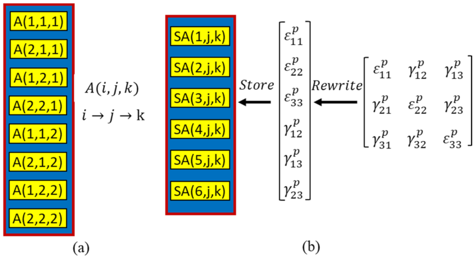
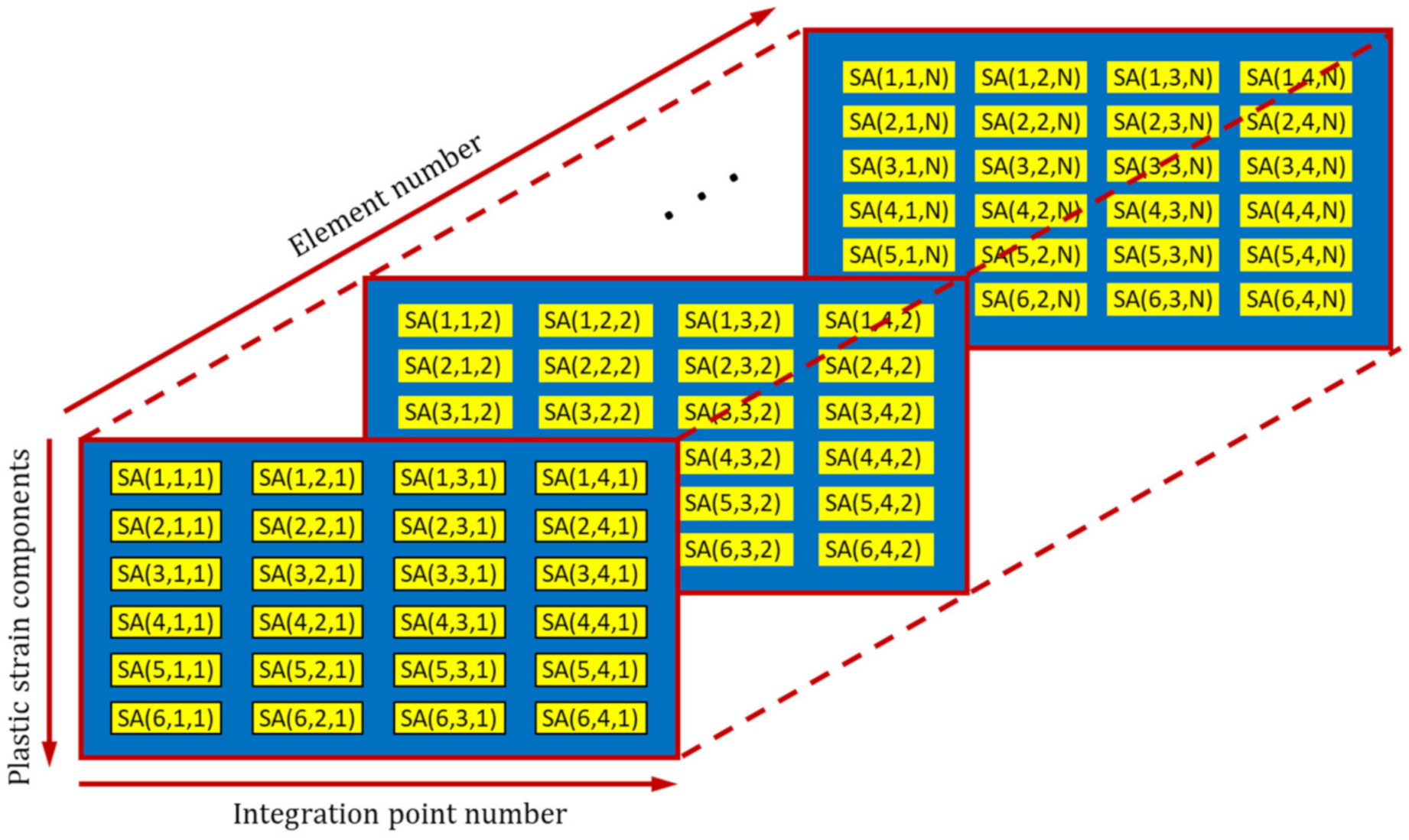
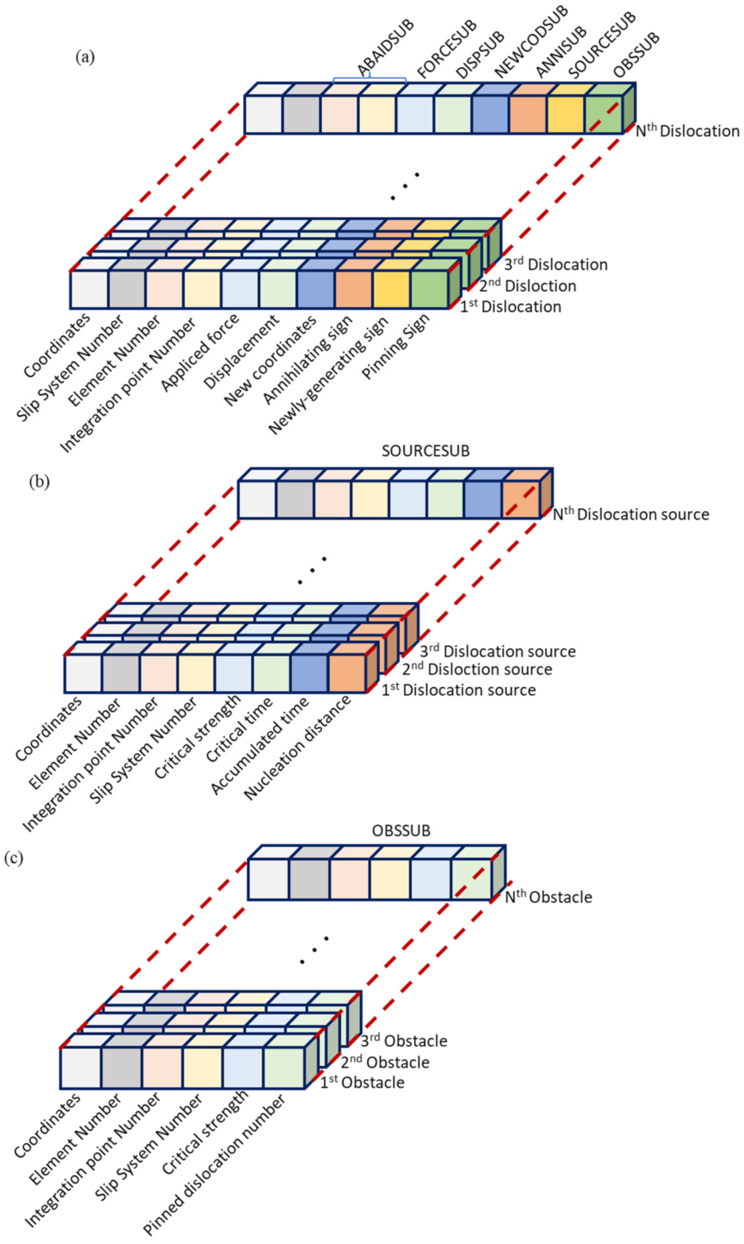
4.2. Data Structure for the Coupling Framework

The data structures of dislocations, obstacles, and dislocation sources are shown in Figure 8. It can be seen that the basic data structure of a dislocation consists of identity number, location information, its sign (i.e., plus or minus one, representing positive or negative dislocations, respectively), and the state information. The information of location includes the coordinate value, the located slip system, and the element and integration point number where the dislocation resides, as shown in Figure 8a. The preliminary calculation with user subroutines generates the stress, displacement, and new coordinates of the dislocation i , and then the state information (i.e., illustrating whether the dislocation is pinned, annihilated, or newly generated) is obtained. Moreover, as can be seen from Figure 8b, the data structure related to dislocation sources and obstacles is much simpler compared to the dislocations. In addition to the location information, the critical strength and time are added for sources and only strength is added for obstacles, as shown in Figure 8c. During the deformation process, these data are read and updated continuously by the self-defined subroutines mentioned in the above section. As shown in Figure 8a, for the dislocation, its relative element and integration point number are updated by the subroutine ABAIDSUB, and the driving force, displacement, and new coordinates are calculated and updated by subroutines FORCESUB, DISPSUB, and NEWCODSUB, respectively. The signs of annihilating, newly generating, and pinning are determined by subroutines ANNISUB, SOURCESUB, and OBSSUB. The data structure of sources is mainly visited and updated by subroutine SOURCESUB. Similarly, the data structure of obstacles is accessed by subroutine OBSSUB.
The initial data structures of dislocations, sources, and obstacles (i.e., the data structures before loading is applied) are utilized to describe the reference state of the DDD module. They are generated by MATLAB and written into text files that are visited at the start of ABAQUS/Standard analysis to initialize the DDD module.

5. Uniaxial Compression Simulation for Single Crystal Micropillar

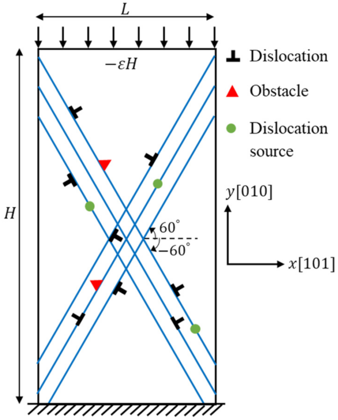
5.1. Computational Model of Micropillars

For verification, the developed simulation model is used to study the deformation behaviors of crystal materials under uniaxial compression. As shown in Figure 9, micropillars with four different widths are built with a constant aspect ratio of height H to width L (H/L = 2). An isotropic aluminum single crystal is considered here with Poisson’s ratio v = 0.3 , shear modulus μ = 26   Gpa , Burgers vector b = 0.25   nm , and drag coefficient B = 10 4   Pa   s [28,44,45].
For face-centered crystal Al, the representative material parameters used in DDD are the same as the ones used in other research [28,30,43,45]. Two slip systems with the interaction angle of ± 60 ° relative to the horizontal direction are considered with the spacing distance of two neighboring slip planes being 10b. This approximates to the active slip systems of the face-centered crystal in plastic strain problems. The x-axis and y-axis represent the crystal directions [101] and [010], respectively. Static dislocation sources are distributed on these slip planes randomly with strength satisfying the Gaussian distribution with mean value 50 MPa and standard deviation 10 MPa. The critical time for dislocation nucleation is set as 10 ns. The obstacles in the model are with mean strength 150 MPa and 20% standard deviation.
To mimic the compression experiment, a fixed compressive strain rate ε ˙ = 1000 / s is imposed for all samples. Time steps of 1   ns for DD and 10   ns for the FEM are used here [49]. In all the simulations, the bottom boundaries of specimens are fixed as:
u x = u y = 0 ,     a t   Y = 0 ,
The upper surface is subjected to a velocity v x such that
v y = L ε ˙ ,   a t   Y = L ,
DCM simulations are performed with the boundary conditions and material parameters as described above. The simulation results are discussed below.

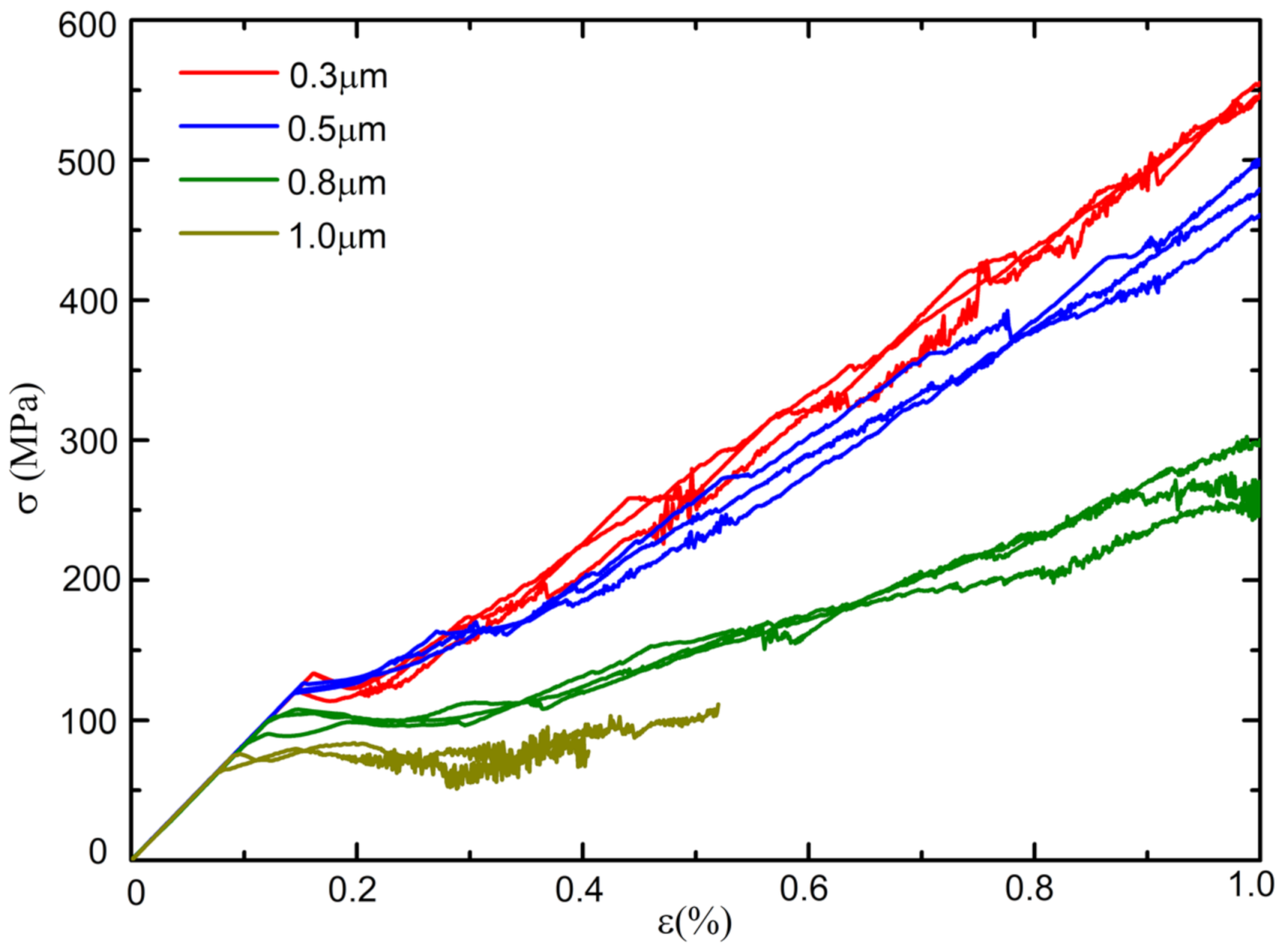
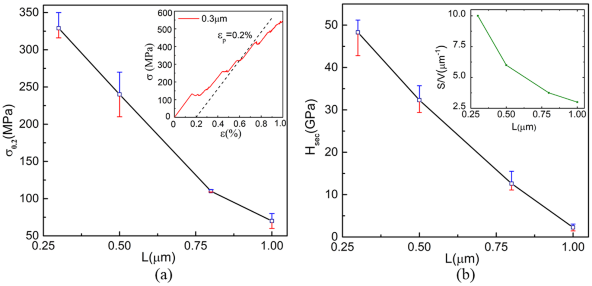
5.2. Effect of Sample Size on Crystal Strength

The computationally obtained σ ~ ε curves are plotted in Figure 10 for four different simple sizes L = 0.3 ,   0.5 , 0.8 , 1.0   μ m . To avoid the potential effect of defect distribution (i.e., the distribution of dislocations, sources, and obstacles) on the simulation results, for each size, three simulations are carried out with different defect distributions. It is found that the smaller the sample size, the higher the strength, as observed in experimental investigation [5]. This validates that the present simulation model is capable of capturing the microscale plastic response. Due to numerous dislocations being greatly active at L = 1.0 μm, the stress–strain curves oscillate poorly and even fail at small strains. A similar phenomenon was also found in the compressing simulation of copper micropillars [50]. From these stress–strain curves, we compute the nominal yield stress σ 0.2 , which is the stress value at 0.2% plastic strain offsets, and plot it in Figure 11a. The inset of Figure 11a shows the acquiring of the normal yield stress for the 0.3 μm-wide micropillar. The results indicate that the yield stress increases with decreasing pillar size. The error bars denote the range of the values of σ 0.2 .
In addition, the secant strain hardening modulus, H s e c , is defined as the ratio of stress to plastic strain from ε p = 0.1 % to ε p = 0.3 % , as follows:
H s e c = σ ε = 0.003 σ ε = 0.001 0.003 0.001 ,
Then, the average value of H s e c over three realizations for a particular pillar size, H a v e , is calculated and plotted in Figure 11b. It shows that the average strain hardening modulus decreases with sample size and that larger pillars are with the smaller scatter of H a v e values. In addition, the ratio of surface area to volume, which is reduced to the ratio of length to surface area for the plane strain problem, is calculated for each pillar. The inset of Figure 11b shows that the ratio decreases with sample size, although all the samples have the same length–width ratio. It indicates that dislocations in small samples have a high possibility to escape from the sample. The escape of dislocations from the free surface can result in the dislocation starvation effect [49] in small pillars and the hardening of materials.

6. Conclusions

In this paper, a concurrent multiscale simulation method is developed to shed light on the material plasticity at the microscale. In this method, the DDD module looks to the FEM module to solve the boundary conditions and the FEM module turns to DDD for plastic strain, which determines the constitutive law of the FEM.
The key issue in the DDD-FEM coupling scheme is how to reasonably regularize the discrete plastic strain to integration points of continuum mechanics. A novel FE mesh-based regularization method is proposed by using a Burgers vector density function and the characteristics of a finite element mesh in ABAQUS. It shows high accuracy and considerably improves the efficiency by avoiding the tedious calculations.
To achieve the concurrent computational model, the DDD module is programmed into Fortran codes, and then it is incorporated into the Abaqus analysis by calling user subroutines provided by Abaqus to determine the constitutive law. The stress field is stored in COMMON blocks and transferred to DDD codes. The realization of the multiscale model capitalizes on the secondary development of FEM software Abaqus, and the implementation details are presented for the first time.
The developed multiscale framework is able to capture the plastic behavior of microscale crystals. Using this multiscale method, uniaxial compression tests of micropillars are performed to study the size effect on plasticity and its underlying mechanisms. The observed secant strain hardening of the modulus and yield stress might be due to the high probability of dislocations in smaller size to escape from the free surface.
This multiscale framework can be potentially employed in studying the plastic behavior of materials with complex microstructures and deeply revealing its underlying mechanisms. In future work, the developed simulation model will consider a variety of complex dislocation motions, such as dislocation climb, interactions between dislocation and grain boundary, and dislocation junction formation.

Author Contributions

Z.Z.: Methodology, investigation, data curation, formal analysis, writing—original draft preparation. Z.T.: Conceptualization, supervision, resources, writing—reviewing and editing, funding acquisition. X.J.: Supervision, project administration, funding acquisition. All authors have read and agreed to the published version of the manuscript.

Funding

The authors would like to acknowledge the funding support from the UK’s EPSRC Future Metrology Hub (Ref: EP/P006930/1), the UK’s STFC Innovation Partnership Scheme (STFC-IPS) project under grant agreement No. ST/V001280/1, and the European Union’s Horizon 2020 research and innovation program under grant agreement No. 767589.

Institutional Review Board Statement

Not applicable.

Informed Consent Statement

Not applicable.

Data Availability Statement

Not applicable.

Acknowledgments

The authors would like to acknowledge the scholarship received from the UK’s EPSRC Future Metrology Hub (Ref: EP/P006930/1) and the China Scholarship Council (CSC) on Zhenting Zhang’s PhD study.

Conflicts of Interest

The authors declare no conflict of interest.

References

  1. Ferretti, E. Shape-effect in the effective laws of plain and rubberized concrete. Comput. Mater. Contin. 2012, 30, 237. [Google Scholar]
  2. Xu, Z.-H.; Li, X. Sample size effect on nanoindentation of micro-/nanostructures. Acta Mater. 2006, 54, 1699–1703. [Google Scholar] [CrossRef]
  3. Hudson, J.; Brown, E.; Fairhurst, C. Shape of the Complete Stress-Strain Curve for Rock. In Proceedings of the 13th Symposium on Rock Mechanics, University of Illinois, Urbana, IL, USA, 30 August–1 September 1971. [Google Scholar]
  4. Brunetaud, X.; Khelifa, M.-R.; Al-Mukhtar, M. Size effect of concrete samples on the kinetics of external sulfate attack. Cem. Concr. Compos. 2012, 34, 370–376. [Google Scholar] [CrossRef]
  5. Takata, N.; Takeyasu, S.; Li, H.; Suzuki, A.; Kobashi, M. Anomalous size-dependent strength in micropillar compression deformation of commercial-purity aluminum single-crystals. Mater. Sci. Eng. A 2020, 772, 138710. [Google Scholar] [CrossRef]
  6. Dunstan, D.J.; Bushby, A.J. The scaling exponent in the size effect of small scale plastic deformation. Int. J. Plast. 2013, 40, 152–162. [Google Scholar] [CrossRef]
  7. Abad, O.T.; Wheeler, J.M.; Michler, J.; Schneider, A.S.; Arzt, E. Temperature-dependent size effects on the strength of Ta and W micropillars. Acta Mater. 2016, 103, 483–494. [Google Scholar] [CrossRef] [Green Version]
  8. Lavenstein, S.; El-Awady, J.A. Micro-scale fatigue mechanisms in metals: Insights gained from small-scale experiments and discrete dislocation dynamics simulations. Curr. Opin. Solid State Mater. Sci. 2019, 23, 100765. [Google Scholar] [CrossRef]
  9. Yuan, S.; Huang, M.; Zhu, Y.; Li, Z. A dislocation climb/glide coupled crystal plasticity constitutive model and its finite element implementation. Mech. Mater. 2018, 118, 44–61. [Google Scholar] [CrossRef]
  10. Cui, Y.; Po, G.; Ghoniem, N. Influence of loading control on strain bursts and dislocation avalanches at the nanometer and micrometer scale. Phys. Rev. B 2017, 95, 064103. [Google Scholar] [CrossRef] [Green Version]
  11. Xie, W.; Fang, F. On the mechanism of dislocation-dominated chip formation in cutting-based single atomic layer removal of monocrystalline copper. Int. J. Adv. Manuf. Technol. 2020, 108, 1587–1599. [Google Scholar] [CrossRef]
  12. Vattré, A.; Devincre, B.; Roos, A.; Feyel, F. Predicting size effects in nickel-base single crystal superalloys with the Discrete-Continuous Model. Eur. J. Comput. Mech. Rev. Eur. Mécanique Numérique 2010, 19, 65–76. [Google Scholar] [CrossRef]
  13. Keralavarma, S.M.; Curtin, W.A. Strain hardening in 2D discrete dislocation dynamics simulations: A new ‘2.5D’ algorithm. J. Mech. Phys. Solids 2016, 95, 132–146. [Google Scholar] [CrossRef] [Green Version]
  14. Chen, G.; Ren, C.; Zhang, P.; Cui, K.; Li, Y. Measurement and finite element simulation of micro-cutting temperatures of tool tip and workpiece. Int. J. Mach. Tools Manuf. 2013, 75, 16–26. [Google Scholar] [CrossRef]
  15. Schulze, V.; Autenrieth, H.; Deuchert, M.; Weule, H. Investigation of surface near residual stress states after micro-cutting by finite element simulation. CIRP Ann. 2010, 59, 117–120. [Google Scholar] [CrossRef]
  16. Ji, H.; Song, Q.; Kumar Gupta, M.; Cai, W.; Zhao, Y.; Liu, Z. Grain scale modelling and parameter calibration methods in crystal plasticity finite element researches: A short review. J. Adv. Manuf. Sci. Technol. 2021, 1, 41–50. [Google Scholar] [CrossRef]
  17. Herrera-Solaz, V.; Cepeda-Jiménez, C.M.; Pérez-Prado, M.T.; Segurado, J.; Niffenegger, M. The influence of underlying microstructure on surface stress and strain fields calculated by crystal plasticity finite element method. Mater. Today Commun. 2020, 24, 101176. [Google Scholar] [CrossRef]
  18. Rousseau, T.; Nouguier-Lehon, C.; Gilles, P.; Hoc, T. Finite element multi-impact simulations using a crystal plasticity law based on dislocation dynamics. Int. J. Plast. 2018, 101, 42–57. [Google Scholar] [CrossRef]
  19. Gurrutxaga-Lerma, B.; Balint, D.S.; Dini, D.; Sutton, A.P. A Dynamic Discrete Dislocation Plasticity study of elastodynamic shielding of stationary cracks. J. Mech. Phys. Solids 2017, 98, 1–11. [Google Scholar] [CrossRef] [Green Version]
  20. Geada, I.L.; Ramezani-Dakhel, H.; Jamil, T.; Sulpizi, M.; Heinz, H. Insight into induced charges at metal surfaces and biointerfaces using a polarizable Lennard–Jones potential. Nat. Commun. 2018, 9, 716. [Google Scholar] [CrossRef]
  21. Zhang, Y.; Cheng, Z.; Lu, L.; Zhu, T. Strain gradient plasticity in gradient structured metals. J. Mech. Phys. Solids 2020, 140, 103946. [Google Scholar] [CrossRef]
  22. Xiao, X.; Yu, L. Cross-sectional nano-indentation of ion-irradiated steels: Finite element simulations based on the strain-gradient crystal plasticity theory. Int. J. Eng. Sci. 2019, 143, 56–72. [Google Scholar] [CrossRef]
  23. Barboura, S.; Li, J. Establishment of strain gradient constitutive relations by using asymptotic analysis and the finite element method for complex periodic microstructures. Int. J. Solids Struct. 2018, 136, 60–76. [Google Scholar] [CrossRef]
  24. Hansen, L.T.; Fullwood, D.T.; Homer, E.R.; Wagoner, R.H.; Lim, H.; Carroll, J.D.; Zhou, G.; Bong, H.J. An investigation of geometrically necessary dislocations and back stress in large grained tantalum via EBSD and CPFEM. Mater. Sci. Eng. A 2020, 772, 138704. [Google Scholar] [CrossRef]
  25. Han, X. Investigate the mechanical property of nanopolycrystal silicon by means of the nanoindentation method. AIP Adv. 2020, 10, 065230. [Google Scholar] [CrossRef]
  26. Li, J.; Lu, B.; Zhang, Y.; Zhou, H.; Hu, G.; Xia, R. Nanoindentation response of nanocrystalline copper via molecular dynamics: Grain-size effect. Mater. Chem. Phys. 2020, 241, 122391. [Google Scholar] [CrossRef]
  27. Lemarchand, C.; Devincre, B.; Kubin, L.P. Homogenization method for a discrete-continuum simulation of dislocation dynamics. J. Mech. Phys. Solids 2001, 49, 1969–1982. [Google Scholar] [CrossRef]
  28. Van der Giessen, E.; Needleman, A. Discrete dislocation plasticity: A simple planar model. Model. Simul. Mater. Sci. Eng. 1995, 3, 689–735. [Google Scholar] [CrossRef]
  29. Benzerga, A.A. Micro-pillar plasticity: 2.5D mesoscopic simulations. J. Mech. Phys. Solids 2009, 57, 1459–1469. [Google Scholar] [CrossRef]
  30. Huang, M.; Li, Z. Coupled DDD–FEM modeling on the mechanical behavior of microlayered metallic multilayer film at elevated temperature. J. Mech. Phys. Solids 2015, 85, 74–97. [Google Scholar] [CrossRef]
  31. Cui, Y.-n.; Liu, Z.-l.; Zhuang, Z. Theoretical and numerical investigations on confined plasticity in micropillars. J. Mech. Phys. Solids 2015, 76, 127–143. [Google Scholar] [CrossRef]
  32. Cui, Y.-n.; Liu, Z.-l.; Wang, Z.-j.; Zhuang, Z. Mechanical annealing under low-amplitude cyclic loading in micropillars. J. Mech. Phys. Solids 2016, 89, 1–15. [Google Scholar] [CrossRef]
  33. Cui, Y.; Po, G.; Ghoniem, N. Temperature insensitivity of the flow stress in body-centered cubic micropillar crystals. Acta Mater. 2016, 108, 128–137. [Google Scholar] [CrossRef] [Green Version]
  34. Hu, J.; Liu, Z.; Chen, K.; Zhuang, Z. Investigations of shock-induced deformation and dislocation mechanism by a multiscale discrete dislocation plasticity model. Comput. Mater. Sci. 2017, 131, 78–85. [Google Scholar] [CrossRef]
  35. Hu, J.-Q.; Liu, Z.-L.; Cui, Y.-N.; Liu, F.-X.; Zhuang, Z. A New View of Incipient Plastic Instability during Nanoindentation. Chin. Phys. Lett. 2017, 34, 046101. [Google Scholar] [CrossRef]
  36. Santos-Güemes, R.; Esteban-Manzanares, G.; Papadimitriou, I.; Segurado, J.; Capolungo, L.; Llorca, J. Discrete dislocation dynamics simulations of dislocation-θ′ precipitate interaction in Al-Cu alloys. J. Mech. Phys. Solids 2018, 118, 228–244. [Google Scholar] [CrossRef] [Green Version]
  37. Huang, S.; Huang, M.; Li, Z. Effect of interfacial dislocation networks on the evolution of matrix dislocations in nickel-based superalloy. Int. J. Plast. 2018, 110, 1–18. [Google Scholar] [CrossRef]
  38. Liu, F.X.; Liu, Z.L.; Pei, X.Y.; Hu, J.Q.; Zhuang, Z. Modeling high temperature anneal hardening in Au submicron pillar by developing coupled dislocation glide-climb model. Int. J. Plast. 2017, 99, 102–119. [Google Scholar] [CrossRef]
  39. Zbib, H.M.; de la Rubia, T.D. A multiscale model of plasticity. Int. J. Plast. 2002, 18, 1133–1163. [Google Scholar] [CrossRef]
  40. Liu, Z.L.; Liu, X.M.; Zhuang, Z.; You, X.C. A multi-scale computational model of crystal plasticity at submicron-to-nanometer scales. Int. J. Plast. 2009, 25, 1436–1455. [Google Scholar] [CrossRef]
  41. Vattré, A.; Devincre, B.; Feyel, F.; Gatti, R.; Groh, S.; Jamond, O.; Roos, A. Modelling crystal plasticity by 3D dislocation dynamics and the finite element method: The Discrete-Continuous Model revisited. J. Mech. Phys. Solids 2014, 63, 491–505. [Google Scholar] [CrossRef]
  42. Cui, Y.; Liu, Z.; Zhuang, Z. Quantitative investigations on dislocation based discrete-continuous model of crystal plasticity at submicron scale. Int. J. Plast. 2015, 69, 54–72. [Google Scholar] [CrossRef]
  43. Song, H.; Yavas, H.; Giessen, E.V.d.; Papanikolaou, S. Discrete dislocation dynamics simulations of nanoindentation with pre-stress: Hardness and statistics of abrupt plastic events. J. Mech. Phys. Solids 2019, 123, 332–347. [Google Scholar] [CrossRef] [Green Version]
  44. Kondori, B.; Needleman, A.; Amine Benzerga, A. Discrete dislocation simulations of compression of tapered micropillars. J. Mech. Phys. Solids 2017, 101, 223–234. [Google Scholar] [CrossRef]
  45. Papanikolaou, S.; Song, H.; Van der Giessen, E. Obstacles and sources in dislocation dynamics: Strengthening and statistics of abrupt plastic events in nanopillar compression. J. Mech. Phys. Solids 2017, 102, 17–29. [Google Scholar] [CrossRef] [Green Version]
  46. Cai, W.; Arsenlis, A.; Weinberger, C.R.; Bulatov, V.V. A non-singular continuum theory of dislocations. J. Mech. Phys. Solids 2006, 54, 561–587. [Google Scholar] [CrossRef]
  47. Huang, M.; Tong, J.; Li, Z. A study of fatigue crack tip characteristics using discrete dislocation dynamics. Int. J. Plast. 2014, 54, 229–246. [Google Scholar] [CrossRef]
  48. Zhou, N.; Elkhodary, K.I.; Huang, X.; Tang, S.; Li, Y. Dislocation structure and dynamics govern pop-in modes of nanoindentation on single-crystal metals. Philos. Mag. 2020, 100, 1585–1606. [Google Scholar] [CrossRef]
  49. Liu, Z.; Liu, X.; Zhuang, Z.; You, X. Atypical three-stage-hardening mechanical behavior of Cu single-crystal micropillars. Scr. Mater. 2009, 60, 594–597. [Google Scholar] [CrossRef]
  50. Akarapu, S.; Zbib, H.M.; Bahr, D.F. Analysis of heterogeneous deformation and dislocation dynamics in single crystal micropillars under compression. Int. J. Plast. 2010, 26, 239–257. [Google Scholar] [CrossRef]
Figure 1. Schematic of the coupling scheme of DCM (Yellow block represents the single element in FEM module.).
Crystals 12 00329 g001
Figure 2. Schematic of distributing plastic strain to integration points of the FEM. The black points represent integration points. The red areas and the shaded areas are the core domains and secondary domains, respectively.
Crystals 12 00329 g002
Figure 3. The numbering of integration points and nodes in 2D quadrilateral parent elements: (a) 4-node element, (b) 4-node reduced integration element, (c) 8-node element, and (d) 8-node reduced integration element. The dashed lines divide the element into integration point domains. The red dot and black cross represent the node and integration point, respectively.
Crystals 12 00329 g003
Figure 4. Schematic of two-dimensional coordinate system conversion. (a) (x, y) and (x′, y′) represent the position of point A in the coordinate system OXY and O′X′Y′, respectively. (b) The transformation matrix R can be obtained from the relationship of two coordinate systems.
Crystals 12 00329 g004
Figure 5. The workflow of the multiscale framework coupling FEM and DCM.
Crystals 12 00329 g005
Figure 6. The storage format of arrays in Fortran (a), and the plastic strain tensor re-written into the vector to store in an array (b).
Crystals 12 00329 g006
Figure 7. The data structure of plastic strain tensor at the integration points of all elements.
Crystals 12 00329 g007
Figure 8. The data structures of dislocations (a), obstacles (b), and dislocation sources (c), and the relative user subroutines.
Crystals 12 00329 g008
Figure 9. Sketch of micropillar compression. The black T-signs represent dislocations. The red triangle and green circle represent obstacle and source, respectively.
Crystals 12 00329 g009
Figure 10. Stress–strain curves of micropillars with different widths L = {0.3, 0.5, 0.8,1.0} µm.
Crystals 12 00329 g010
Figure 11. The yield stress at 0.2% plastic strain offsets, σ 0.2 , (a) and average secant hardening modulus, H a v e , (b) versus the width of micropillars. The inset in (a) shows the capture of the yield stress from the one stress–strain curve, and the inset in (b) is the ratio of surface area to volume for each micropillar.
Crystals 12 00329 g011
Table 1. Gauss numerical integration constants.
Number of Integration Points (n) Integration   Point   Location   x i
1 x 1 = 0
2 x 1 = 1 / 3 ,   x 2 = 1 / 3
3 x 1 = 0.6 ,   x 2 = 0 ,   x 3 = 0.6
Publisher’s Note: MDPI stays neutral with regard to jurisdictional claims in published maps and institutional affiliations.

