Influence of Fault Current and Different Oscillating Magnetic Fields on Electromagnetic–Thermal Characteristics of the REBCO Coil

Abstract

When the high-temperature superconducting (HTS) REBCO (rare-earth barium copper oxide) coil is applied in a power system, a large amount of heat may be generated due to the short-circuiting of the system, resulting in the thermal instability of the coil. Moreover, under complex working conditions, the oscillating external magnetic field will further aggravate the coil quench. In this paper, the electromagnetic–thermal coupling model is used to analyze the loss, current distribution and temperature distribution of the REBCO coil under short-circuit fault conditions and oscillating external magnetic fields. In order to get closer to the actual situation, the modeling of the superconducting tape adopts the real tape structure, and the resistivity of the superconductor is described by the modified E-J relationship. Four cases are considered for the oscillating external magnetic field, i.e., sine, triangle, sawtooth and square cases. This model has certain significance as a reference for understanding the thermal stability of coils in extreme cases.

1. Introduction

High-temperature superconducting (HTS) coils are widely used in superconducting generators, superconducting transformers, superconducting fault current limiters (SFCLs), superconducting magnetic energy storage (SMES) and wireless power transmission (WPT) [1,2,3,4,5]. In some extreme cases, such as the most serious fault of a three-phase short circuit in a superconducting generator, the superconducting coil will experience a large fault current. The coil will generate a large amount of loss when the fault current impacts, and the loss will cause the temperature of the tape to rise, thus causing the performance of the tape to decline or even tape damage [1,2,3,6,7]. In addition, under actual application conditions, the superconducting coil may be in a complex dynamic external field, and the superconducting magnet may also generate loss under the external field, thus affecting the thermal stability of the system [8,9,10,11]. Therefore, it is very important to study the electromagnetic and thermal properties of superconducting coils under complex oscillating external fields and fault currents.

Some researchers have reported loss and temperature information for superconducting coils under fault currents or complex magnetic fields. Chen et al. studied the current and temperature distribution of the superconducting coil in an SFCL under fault current conditions by combining experiments with finite element simulation. Finite element simulation can be used to study some serious fault conditions that are difficult or impossible to realize in experiments [3]. Inoue et al. reported the thermal characteristics of a superconducting coil in the WPT in the kHz band. The AC loss in the HTS coil increases with the increase in frequency, so that the surface temperature of the coil increases and the critical current of the coil decreases [5]. The transient loss and temperature distribution of a superconducting coil under pulse overcurrent conditions are reported in [7]. Ahmadpour et al. studied the electromagnetic and thermal characteristics of a superconducting transformer coil wound with Bi-2223 tape under short-circuit fault conditions. The results showed that the coil had good thermal stability [12]. In the case of external magnetic fields, Glowacki et al. reported the influence of magnetic ripple fields on the coil loss and temperature of an AC motor [10]. Shen et al. reported the effect of oscillating external magnetic fields on the AC loss and dynamic resistance of HTS tapes, but the temperature characteristics have not been studied [8,9]. In addition, under fault currents and oscillating external fields, the local current density of a superconductor may exceed by several times the critical current density. In such cases, the E-J relationship generally used to describe the resistivity of the superconductor will not be applicable, because the resistivity of the superconductor will not increase without limitation with the increase in the current density. Therefore, it is necessary to use the modified E-J relationship to describe the resistivity of superconductors [13,14].

In this paper, we use the two-dimensional axisymmetric model of electromagnetic thermal coupling to study the loss and temperature distribution of a superconducting coil under fault current and complex oscillating magnetic field conditions. The complex oscillating magnetic field waveform includes four cases, i.e., sine, triangle, sawtooth and square cases. The research has certain significance as a reference for understanding the electromagnetic and thermal stability of superconducting coils in some extreme cases.

2. Numerical Model and Method

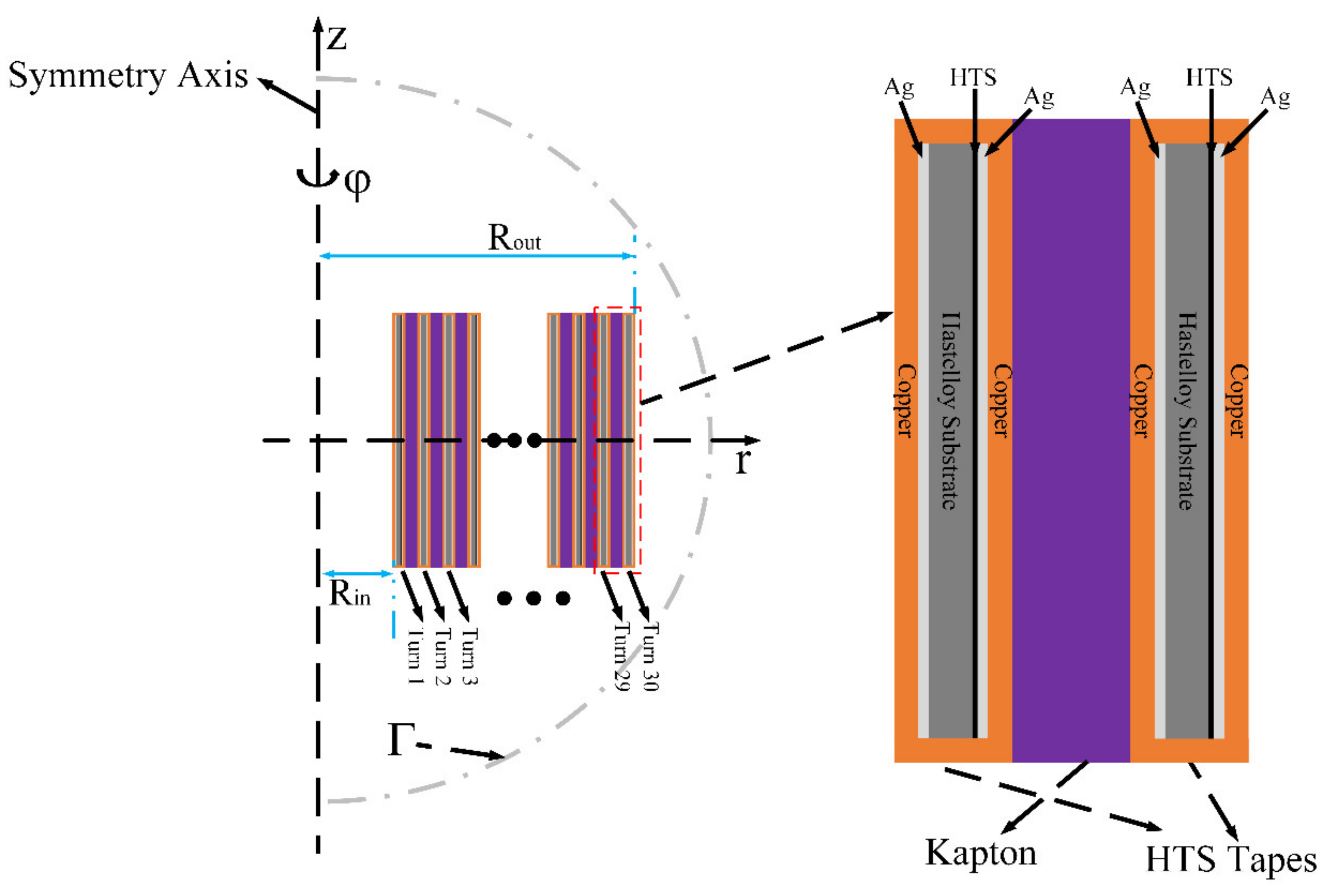
2.1. Geometrics of the HTS Coil

Figure 1 is a two-dimensional axisymmetric model of a cross section of the HTS coil. The coil contains 30 turns in total, and the tapes are insulated with Kapton. The REBCO tape is a typical non-magnetic substrate tape (for example, the tapes manufactured by SuperPower Inc.). The geometric dimensions of the tape and the insulation layer are shown in

Table 1. Parameters of the REBCO and Kapton tapes.

Parameters	REBCO	Kapton
Superconductor width (mm)	4	N.A.
Superconductor thickness (μm)	1	N.A.
Silver layer thickness (μm)	2	N.A.
Substrate thickness (μm)	50	N.A.
Copper layer width (mm)	4.04	N.A.
Copper layer thickness (μm)	20	N.A.
Insulation layer thickness (mm)	N.A.	0.2 [15]
Insulation layer width (mm)	N.A.	4.04

. The inner radius R_in and the outer radius R_out of the coil are 20 mm and 28.65 mm, respectively. The coil is numbered from the innermost layer to the outermost layer: turn 1, turn 2, turn 3, …, turn 29, turn 30.

2.2. Model Description

The loss of the HTS coil was analyzed by H-formulation in COMSOL Multiphysics software [16,17,18,19]. The general form H-formulation is shown in Equation (1) below:

$$\frac{\partial \left({\mu }_0{\mu }_{\mathrm{r}}\mathit{H}\right)}{\partial t}+\nabla \times \left(\rho \nabla \times \mathit{H}\right)=0$$

(1)

where H is the magnetic field strength, µ₀ = 4π × 10⁻⁷ H/m is the permeability in vacuum and µ_r is the relative permeability. In this paper, because magnetic materials are not considered, µ_r = 1.

The magnetic flux density B and the current density J can be expressed by the following Equations (2) and (3):

$$\mathit{B}={\mu }_0{\mu }_{\mathrm{r}}\mathit{H}$$

(2)

$$\nabla \times \mathit{H}=\mathit{J}$$

(3)

In the two-dimensional axisymmetric model, H = [H_r, H_z]^T, and the applied current flows in the φ direction. So, J = J_φ and E_φ = ρJ_φ. Equation (1) can be rewritten to give the following Equation (4):

$$\left[\frac{-\frac{\partial \rho \left(\frac{\partial H_r}{\partial z}-\frac{\partial H_z}{\partial r}\right)}{\partial z}}{\frac{1}{r}\frac{\partial \left(r\rho \left(\frac{\partial H_r}{\partial z}-\frac{\partial H_z}{\partial r}\right)\right)}{\partial r}}\right]=\left[\frac{-{\mu }_0\left(\frac{\partial {\mu }_{\mathrm{r}}}{\partial t}{H}_r+{\mu }_{\mathrm{r}}\frac{\partial H_r}{\partial t}\right)}{-{\mu }_0\left(\frac{\partial {\mu }_{\mathrm{r}}}{\partial t}{H}_z+{\mu }_{\mathrm{r}}\frac{\partial H_z}{\partial t}\right)}\right]$$

(4)

where ρ is the resistivity of the material. For superconductors, the E-J power exponential relationship is generally used to describe the resistivity. However, under fault current conditions, the fault current peak value is large and exceeds the critical current of superconductors by several times. Therefore, the modified E-J relationship is used to describe the resistivity of the superconductor, as show in Equation (5) [13,14]:

$${\rho }_{sc}=\left\{\begin{array}{c}\frac{{\rho }_{\mathrm{s}}\cdot {\rho }_{\mathrm{normal}}}{{\rho }_{\mathrm{s}}+{\rho }_{\mathrm{normal}}},T<T_c\\ {\rho }_{\mathrm{normal}},T⩾T_c\end{array}\right.$$

(5)

where ${\rho }_{\mathrm{s}}=\frac{E_{\mathrm{c}}}{J_{\mathrm{c}0}\left(\mathit{B},T\right)}{\left(\frac{J}{J_{\mathrm{c}0}\left(\mathit{B},T\right)}\right)}^{n-1}$, $J_{\mathrm{c}0}\left(\mathit{B},T\right)=J_{\mathrm{c}0}\cdot J_{\mathrm{c}}\left(\mathit{B}\right)\cdot J_{\mathrm{c}}\left(T\right)$, ρ_normal = 3.5 × 10⁻⁶ Ω·m, E_c = 1 µV/cm, n = 32 and J_c0 = 2.85 × 10¹⁰ A/m² is the critical current density of REBCO tape under 77 K self-field, that is, the critical current of the tape is I_c0 = 114 A. J_c(B) is the coefficient representing the influence of the magnetic field on critical current density, and J_c(T) is the coefficient representing the influence of temperature on critical current density, as shown in Equations (6) and (7) [20,21]:

$$J_c\left(\mathit{B}\right)=\frac{1}{{\left(1+\sqrt{k^2{B}_{\mathrm{para}}{}^2+B_{\mathrm{perp}}{}^2}/B_0\right)}^{\alpha }}$$

(6)

where B_para and B_perp are magnetic flux density parallel to and perpendicular to the tape surface, respectively. k, B₀ and α are three parameters related to materials, which are equal to 0.25, 52.5 mT and 0.7, respectively [22].

$$J_c\left(T\right)=\left\{\begin{array}{c}1,T⩽T_0\\ \frac{T_{\mathrm{c}}-T}{T_{\mathrm{c}}-T_0},T_0<T<T_{\mathrm{c}}\\ 0,T⩾T_{\mathrm{c}}\end{array}\right.$$

(7)

where T₀ = 77 K is the initial temperature of the coil in liquid nitrogen and T_c = 92 K is the critical temperature, beyond which the superconductor will completely lose its superconductivity. The resistivities of other conventional metal layers vary with temperature [23,24,25].

Each turn of the coil is applied with a fault transport current of the same magnitude, which is applied by a “Pointwise Constraint” in COMSOL, as shown in Equation (8):

$$I_{\mathrm{fc}}\left(t\right)=-I_{\mathrm{p}}\cos \left(2\pi ft\right)+I_{\mathrm{p}}\exp \left(-t/0.1\right)={{\displaystyle \int }}_S{J}_{\mathsf{\phi }}\left(t\right)dS$$

(8)

where I_p is the periodic component of the three-phase short-circuit current, S is the cross section of the tape and f = 50 Hz.

The oscillating external magnetic field is applied to the external boundary Γ through the Dirichlet boundary condition, as shown in Figure 1, and the normalized external magnetic field waveform is shown in Figure 2. In this paper, the amplitude of the external magnetic field is set to 0.5 T, and the direction of the external magnetic field is perpendicular to the coil axis.

After the electromagnetic relationship is established, the calculated loss can be used as the heat source of the heat-transfer module to calculate the temperature distribution. The temperature will change the critical current density of J_c0(B, T) in the electromagnetic module, thus realizing the electromagnetic–thermal coupling.

The governing equation of the thermal module is shown in Equation (9), below [5,20]:

$$dC\frac{\partial T}{\partial t}=\nabla \cdot (k\nabla T)+q$$

(9)

where d is the mass density and C and k are the heat capacity and thermal conductivity, respectively, and their values depend on the temperature [23,24,25]. q = E · J, and the value is calculated by the electromagnetic module.

The heat exchange between the HTS coil and the surrounding liquid nitrogen environment is realized by the heat-transfer boundary conditions, as shown in the following Equation (10) [5,20]:

$$Q=h\left(T_{\mathrm{ext}}-T\right)$$

(10)

where Q is the heat transfer between liquid nitrogen and the surface of the HTS coil, and T_ext = 77 K is the temperature of the liquid nitrogen surrounding the HTS coil. h is the heat transfer coefficient, which is set as 800 W/m²/K in this paper [20].

The loss of the REBCO coil is calculated using Equation (11) [15,16,17]:

$$Q_i=2{{\displaystyle \int }}_0^{0.3}dt{{\displaystyle \int }}_{{\mathsf{\Omega }}_i}\left(2\pi r{E}_{\phi }{J}_{\phi }\right)d\mathsf{\Omega }$$

(11)

where Ω_i is the domain of interest. For conventional metals, Q_i stands for eddy current loss, and for superconductors, Q_i stands for hysteresis loss.

3. Result and Discussion

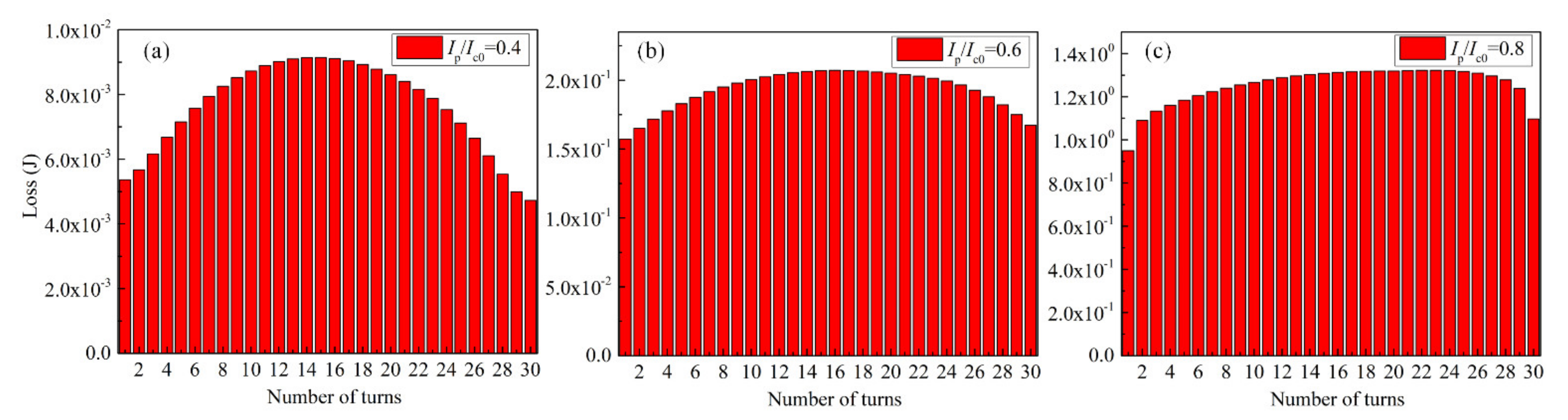
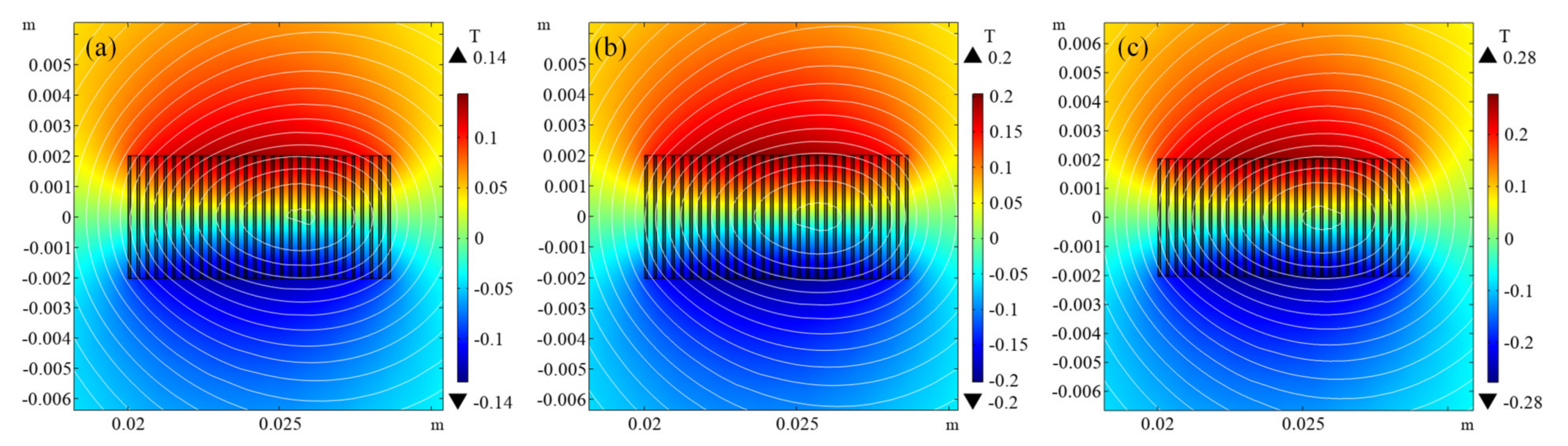
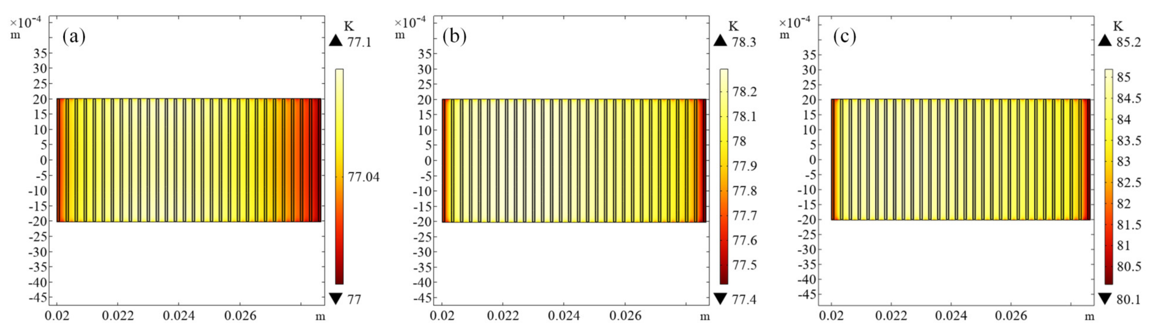
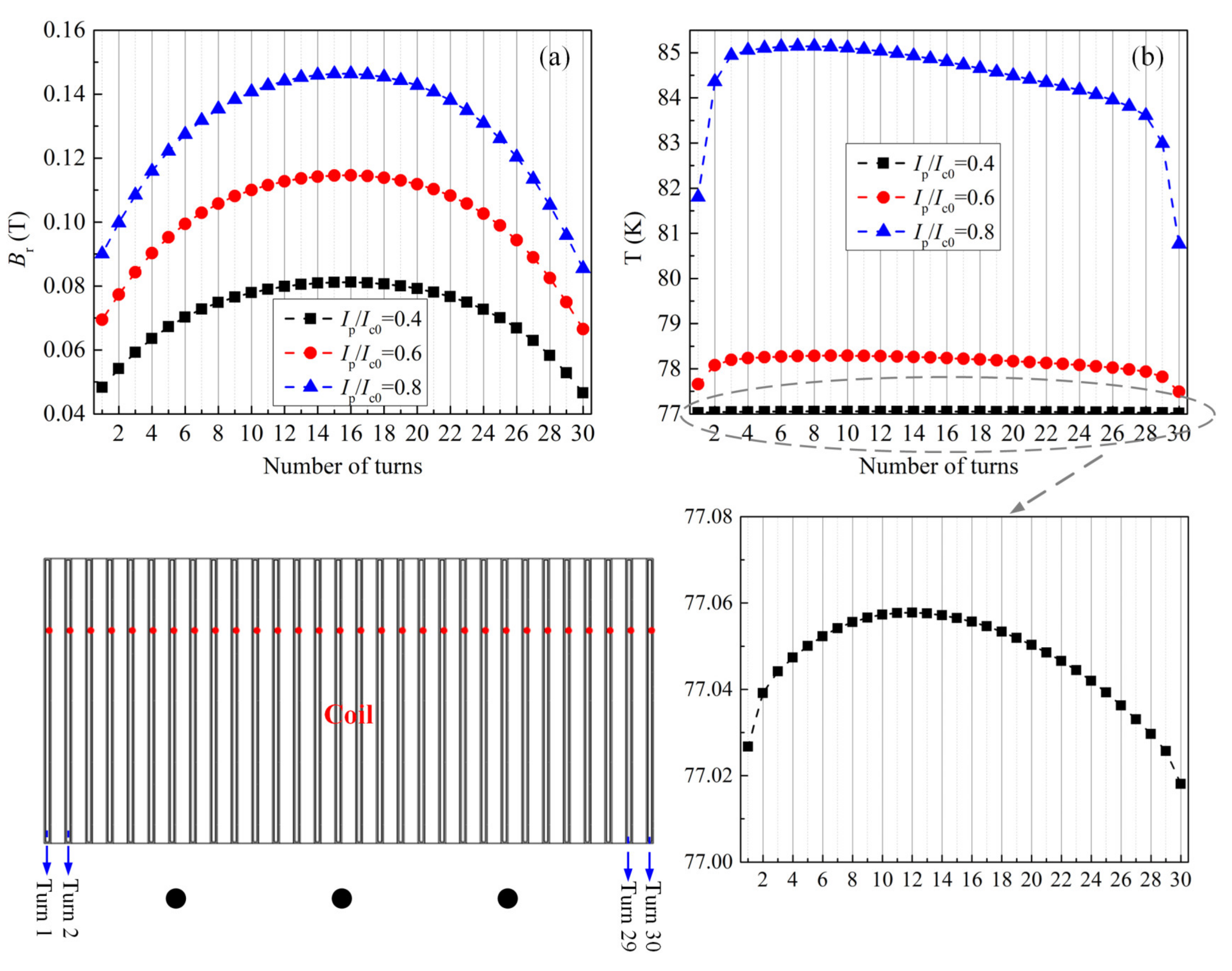
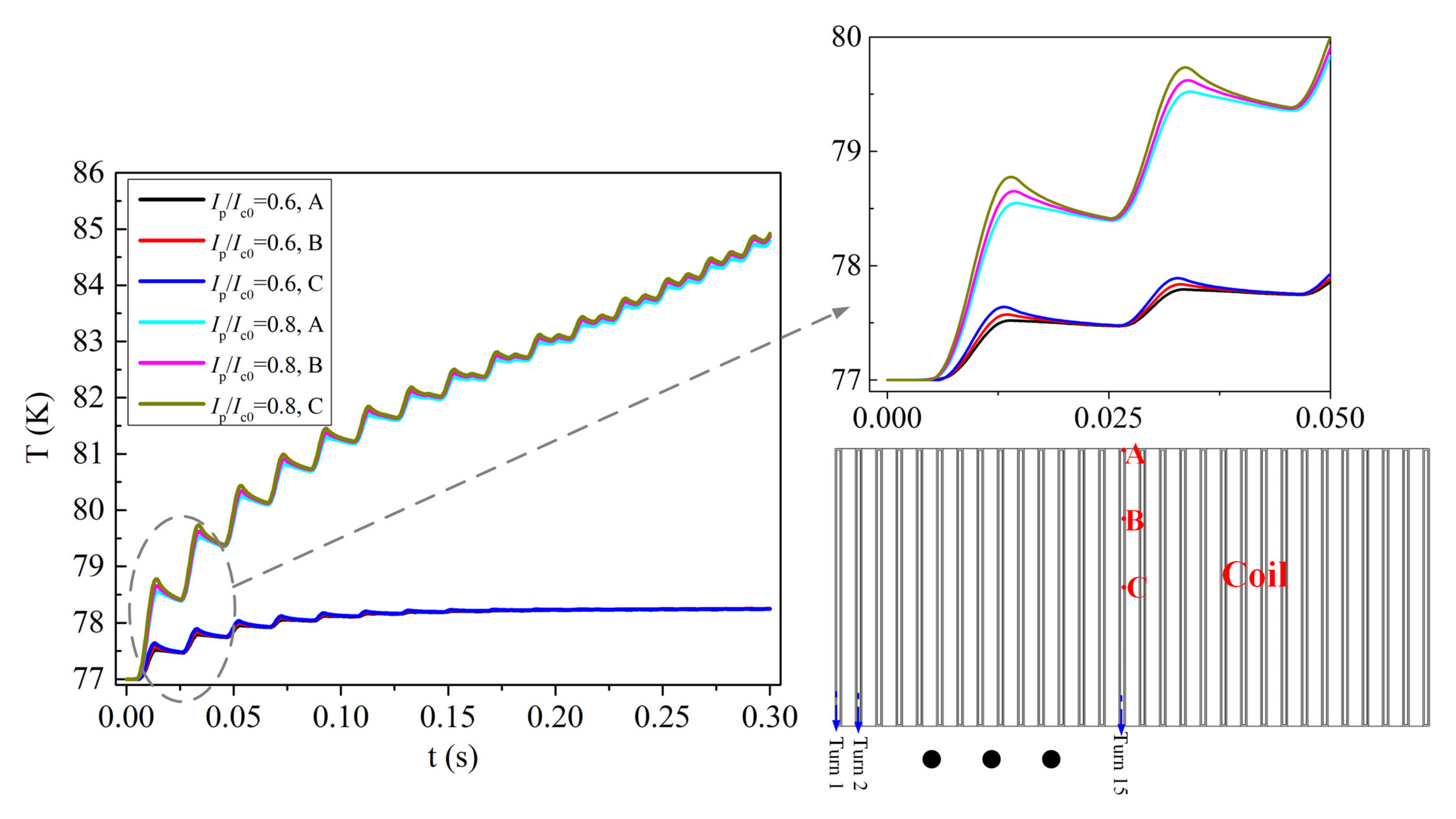
3.1. Loss and Temperature Change during Fault Current Conditions at Self-Field

Figure 3 shows the loss distribution of different layers in the REBCO coil under fault currents of different magnitudes. With the increase in fault current, the loss of different layers gradually increases, and the loss of the metal layer (including the copper layer, the silver layer and the substrate layer) accounts for an increasing proportion of the total loss of the coil. This is because more current flows to the metal layer under higher fault currents, which can be seen in Figure 4. In addition, it can be seen that under different fault currents the copper layer in the metal layer has the largest loss, followed by the silver layer and the substrate layer.

Figure 4 shows the current distribution in different layers of the first turn of the REBCO coil under different transport fault currents, where 4a is I_p/I_c0 = 0.6 and 4b is I_p/I_c0 = 0.8. It can be seen from Figure 4a that the total current in the first turn is carried by the superconducting layer first. When the total current rises to point P in Figure 4a, it starts to drop slightly. At this time, the current intensity carried by the copper layer gradually increases. When the peak value of the fault transport current reaches the maximum value, the total transport current is mainly carried by the superconducting layer and the copper layer, and the silver layer also carries a small part of the current. According to the E-J relationship describing the resistivity of superconductors, the above shunt phenomenon is caused by the increase in the resistivity of the superconducting layer at a higher fault transport current. As the time of the fault current passing through the coil becomes longer, due to the attenuation of the non-periodic component of the fault current, the peak value of the fault current gradually decreases, and finally the total current is almost only carried by the superconducting layer. Different from the situation in Figure 4a, the steady-state fault current in Figure 4b is still large, as shown in the partially enlarged view in Figure 4b. Therefore, when the steady-state fault current flows through the first turn of the superconducting coil, it is mainly carried by the superconducting layer and the copper layer. The difference in current flowing in the different layers of the coil under different strength fault currents will cause obvious differences in loss in the different layers.

As shown in Figure 5, the instantaneous loss in different layers in the coil varies with time under fault currents of different intensities. In Figure 5a, I_p/I_c0 = 0.6, in the initial few cycles, the total loss of the coil comes from the superconducting layer and the copper layer. When the steady-state fault current is reached, the total loss of the coil mainly comes from the superconducting layer, as shown in the partially enlarged view in Figure 5a. Figure 5b shows I_p/I_c0 = 0.8, during the first few cycles of the transport fault current, and during the positive cycle (the transport current value is positive), the total loss of the coil is from the loss in the copper layer and the superconducting layer. During the negative cycle (the transport current value is negative), the total instantaneous loss of the coil is very small. With the passage of fault transport current time, the non-periodic component of the fault current gradually attenuates, and the fault current gradually tends to become a steady fault current. As shown in the locally enlarged view of Figure 5b, at this time, the difference between the instantaneous loss in the negative cycle and the instantaneous loss in the positive cycle gradually decreases. However, when I_p/I_c0 = 0.8, the periodic component of the fault current is large, and the total instantaneous loss of the coil still comes from the superconducting layer and the copper layer.

Figure 6 shows the loss in each turn of the coil under different strength fault currents, where (a) is I_p/I_c0 = 0.4, (b) is I_p/I_c0 = 0.6 and (c) is I_p/I_c0 = 0.8. It can be seen intuitively that under low transport current conditions, the loss in the middle turn of the coil is significantly greater than that in the inner and outer edge turns. Under a high transport current, the loss differences between the middle turns and the inner- and outer-edge turns of the coil are small, and the reason can be given qualitatively by reference to Figure 7, Figure 8 and Figure 9.

Figure 7 shows the distribution of magnetic force lines and radial magnetic flux densities in coil space under fault currents of different intensities at t = 0.01 s (when the short-circuit current reaches the impulse current). Figure 8 shows the distribution of coil temperature under different strengths of fault current when t = 0.3 s, where (a), (b) and (c) correspond to I_p/I_c0 = 0.4, I_p/I_c0 = 0.6 and I_p/I_c0 = 0.8, respectively. Figure 9a shows the change in radial magnetic flux density with coil turns under different fault current intensities at t = 0.01 s, and Figure 9b shows the change in temperature with coil turns under different fault current intensities at t = 0.3 s. The magnetic flux density and temperature collected are shown in the red dot in the lower left figure of Figure 9.

At a low transport current (e.g., I_p/I_c0 = 0.4), the temperature of the coil changes very little, and the heat generated by the coil is taken away by the external liquid nitrogen. As shown in Figure 8a, the maximum temperature of the coil at this time is 77.1 K, so the influence of temperature on the critical current density of the tape in the coil can be ignored. At this time, the critical current density of the tape in the coil is mainly affected by the magnetic field. Due to the anisotropy of the tape, the magnetic field perpendicular to the surface of the tape has the most significant impact on the critical current density of the tape, and thus has the largest impact on the loss [26,27]. Therefore, it can be seen from the radial magnetic flux density distribution in Figure 7a that the radial magnetic flux density of the middle turn of the coil penetrates the deepest, so the loss of the middle turn is significantly greater than the loss of the inner- and outer-edge turns. The quantitative analysis of radial flux density changes with coil turns is shown in Figure 9a. When I_p/I_c0 = 0.4, the radial flux density of the middle turn is the largest, so its loss is the largest.

Under high transport currents (e.g., I_p/I_c0 = 0.8), the temperature rise in the coil is very significant. As shown in Figure 8c, the maximum temperature of the coil reaches 85.2 K. At this time, the influence of temperature on the critical current density of the tape in the coil cannot be ignored. Combined with the radial magnetic flux density distribution in the coil space in Figure 7c, the combined effect of the two (J_c0(B, T)) on the critical current density of the tape in the coil makes the loss distribution at the middle turn of the coil more uniform. The blue curve in Figure 9a,b shows the changes in radial magnetic flux density and temperature with coil turns when I_p/I_c0 = 0.8. Although the maximum value for the radial magnetic flux density still appears in the middle turn, the maximum value of temperature is not in the middle turn, so the maximum loss in the coil does not appear in the middle turn.

Figure 10 shows the temperature changes with time at the 15th turn positions A, B and C of the coil under different fault currents. The three measuring points A, B and C are located in the superconducting layer of the tape, at the 15th turn of the coil. Under a low transport current, i.e., I_p/I_c0 = 0.6, the temperature of the coil will rise within about 0.1 s after the short-circuit fault occurs, and then the heat generated by the coil and the external heat exchange will reach a balance, and the temperature of the coil will not rise further. The temperature rise at position C is higher than those at positions A and B because position C is located at the most central position of the coil, and it is more difficult to exchange heat with the outside. At a high transport current, i.e., I_p/I_c0 = 0.8, the temperature of the coil has been rising within 0.3 s. This is because the heat generated by the coil is greater than the external cooling capacity. It can be predicted that, with further increase in the current passing time, the temperature will exceed the critical temperature of the high-temperature superconductor by 92 K. Therefore, the circuit breaker needs to cooperate to cut off the circuit in time.

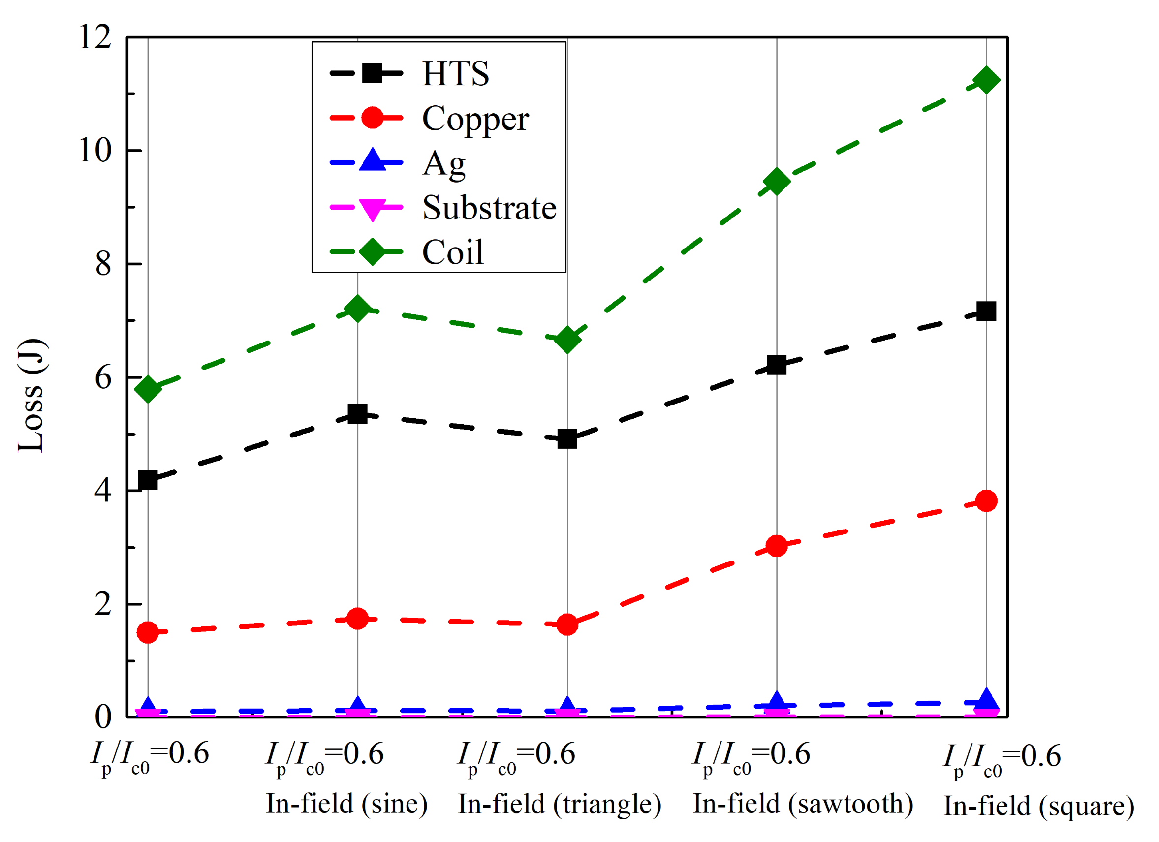
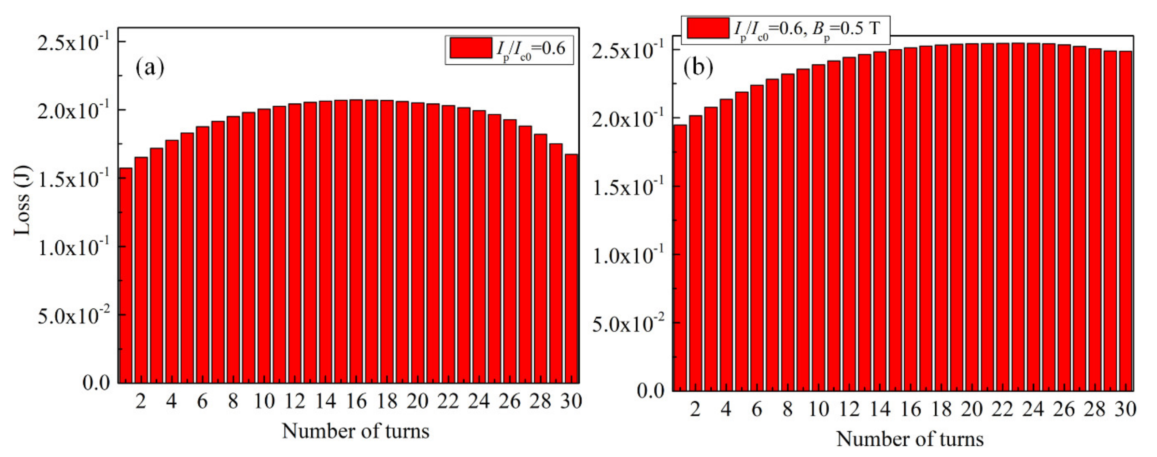
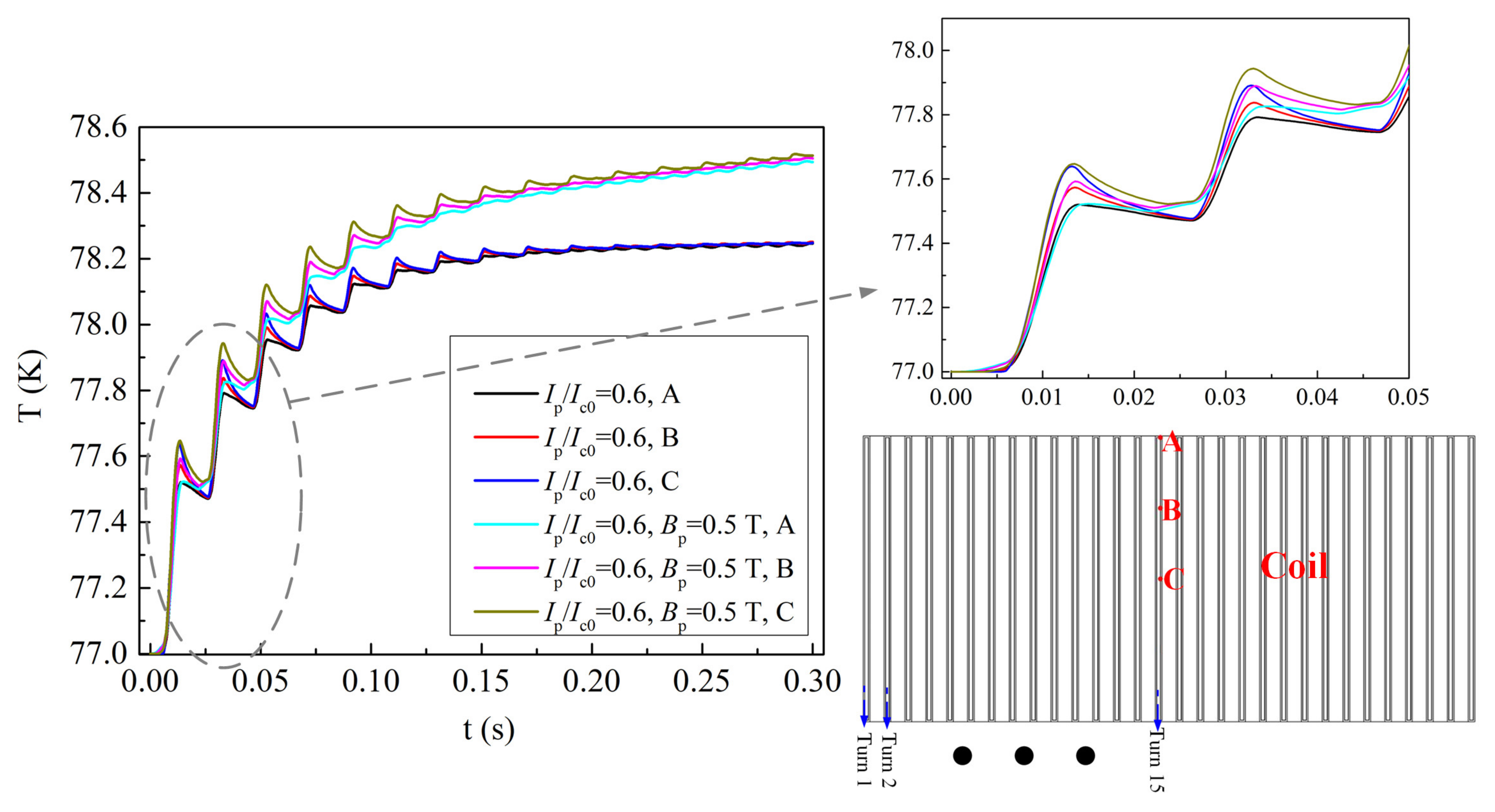
3.2. Loss and Temperature Change during Fault Current Conditions at In-Field

Figure 11 shows the change in the loss of the whole coil and different layers under the self-field and different external oscillating magnetic fields when I_p/I_c0 = 0.6 and the peak value of the external magnetic field B_p = 0.5 T. It can be seen that when there is an external oscillating magnetic field, the loss of the coil will increase. Secondly, although the amplitude of the external oscillating magnetic field is the same, the loss of the coil will also be different when the waveform is different. When the waveform of the oscillating magnetic field is a square wave, the loss of the coil is the largest.

Figure 12 shows the loss distribution for each turn in the coil under two different working conditions. Figure 12a represents the coil only transmitting a fault current (I_p/I_c0 = 0.6). Figure 12b represents the coil transmitting a fault current (I_p/I_c0 = 0.6) and placed in the alternating sine wave background magnetic field (B_p = 0.5 T). It can be seen that the number of turns in the coil with the maximum loss under these two conditions is different. Under the condition of only transport fault current, the number of turns with the maximum loss is 16. When there is a background magnetic field, the number of turns with the maximum loss is 23. This difference is caused by the interaction of the transport current and the shielding current.

Figure 13 shows the temperature change over time at positions A, B and C of the 15th turn of the coil with and without the sine wave background magnetic field under the same fault current. It can be seen that the temperature is higher in the presence of the background magnetic field, which is also due to the increased loss of the coil caused by the background magnetic field. Therefore, under extreme fault conditions, it is still necessary to consider the influence of the background magnetic field on the coil.

4. Conclusions

In this paper, we have studied the effects of fault currents of different magnitudes and different external oscillating magnetic fields on the loss and temperature distribution of the REBCO coil. When the fault current is transmitted, because the fault current peak exceeds the critical current of the tape in the coil, the fault current will be shunted in the tape, which will cause large losses. When the fault current I_p reaches 0.8I_c0, the coil will be thermally quenched. Secondly, at low fault currents, due to the small temperature rise in the coil, the differences between different turn losses in the coil are mainly due to the influence of the magnetic field on tape loss. The magnetic field of the coil middle turn perpendicular to the tape surface is strong, so the middle turn loss is greater than the edge turn loss. Moreover, the difference in the middle turn loss of the coil will be reduced under a large fault current, which is the result of the joint influence of temperature and magnetic field. Under different external oscillating magnetic fields, compared with sinusoidal waveforms, triangular waveforms and sawtooth waveforms, square waveforms have the largest influence on coil loss. Although the fault current is very high, the existence of the external magnetic field still has a certain impact on the coil’s loss and temperature rise. These conclusions have certain significance in providing a reference for the thermal stability design of coils under extreme conditions.

References

1. Baez-Munoz, A.; Trillaud, F.; Rodriguez-Rodriguez, J.R.; Castro, L.M.; Escarela-Perez, R. Thermoelectromagnetic lumped-parameter model of High Temperature Superconductor generators for transient stability analysis. IEEE Trans. Appl. Supercond. 2021, 31, 5201705. [Google Scholar] [CrossRef]
2. Yazdani-Asrami, M.; Staines, M.; Sidorov, G.; Davies, M.; Bailey, J.; Allpress, N.; Glasson, N.; Gholamian, S.A. Fault current limiting HTS transformer with extended fault withstand time. Supercond. Sci. Technol. 2019, 32, 035006. [Google Scholar] [CrossRef]
3. Chen, X.; Gou, H.; Chen, Y.; Jiang, S.; Zhang, M.; Pang, Z.; Shen, B. Superconducting fault current limiter (SFCL) for a power electronic circuit: Experiment and numerical modelling. Supercond. Sci. Technol. 2022, 35, 045010. [Google Scholar] [CrossRef]
4. Chen, X.; Zhang, M.; Jiang, S.; Gou, H.; Zhou, P.; Yang, R.; Shen, B. Energy reliability enhancement of a data center/wind hybrid DC network using superconducting magnetic energy storage. Energy 2023, 263, 125622. [Google Scholar] [CrossRef]
5. Inoue, R.; Ueda, H.; Kim, S.; Tsuda, M. Thermal characteristics of REBCO coil in a wireless power transmission system for the railway vehicle in liquid nitrogen. IEEE Trans. Appl. Supercond. 2021, 31, 4700905. [Google Scholar] [CrossRef]
6. Wu, J.; Tan, Y.; Luo, S.; Hei, Y. Study on Energy Dissipation Mechanism of HTS Tapes in the Impact and Recovery Process. IEEE Trans. Appl. Supercond. 2022, 32, 5600408. [Google Scholar] [CrossRef]
7. Zeng, L.; Chen, X.-Y.; Feng, Y.-J.; Chen, Y.; Xie, Q. Temperature field simulations of a ReBCO pancake coil under pulsed overcurrent conditions. IEEE Trans. Appl. Supercond. 2019, 29, 5900305. [Google Scholar] [CrossRef]
8. Shen, B.; Li, C.; Geng, J.; Dong, Q.; Ma, J.; Gawith, J.; Zhang, K.; Li, Z.; Chen, J.; Zhou, W.; et al. Power dissipation in the HTS coated conductor tapes and coils under the action of different oscillating currents and fields. IEEE Trans. Appl. Supercond. 2019, 29, 8201105. [Google Scholar] [CrossRef]
9. Shen, B.; Chen, X.; Fu, L.; Hao, L.; Coombs, T. Numerical Modelling of the Dynamic Voltage in HTS Materials under the Action of DC Transport Currents and Different Oscillating Magnetic Fields. Materials 2022, 15, 795. [Google Scholar] [CrossRef]
10. Glowacki, J.; Sun, Y.; Storey, J.G.; Huang, T.; Badcock, R.; Jiang, Z. Temperature Distribution in the Field Coil of a 500-kW HTS AC Homopolar Motor. IEEE Trans. Appl. Supercond. 2022, 32, 5200108. [Google Scholar] [CrossRef]
11. Zhang, H.; Wen, Z.; Grilli, F.; Gyftakis, K.; Mueller, M. Alternating current loss of superconductors applied to superconducting electrical machines. Energies 2021, 14, 2234. [Google Scholar] [CrossRef]
12. Ahmadpour, A.; Dejamkhooy, A. Modeling and Analysis of HTS Distribution Transformers Under Various Conditions Using FEM. J. Supercond. Nov. Magn. 2022, 35, 1847–1856. [Google Scholar] [CrossRef]
13. Duron, J.; Grilli, F.; Dutoit, B.; Stavrev, S. Modelling the E–J relation of high-Tc superconductors in an arbitrary current range. Phys. C 2004, 401, 231–235. [Google Scholar] [CrossRef]
14. Xia, J.; Zhou, Y. Numerical simulations of electromagnetic behavior and AC loss in rectangular bulk superconductor with an elliptical flaw under AC magnetic fields. Cryogenics 2015, 69, 1–9. [Google Scholar] [CrossRef]
15. Niu, M.; Yong, H.; Xia, J.; Zhou, Y. The effects of ferromagnetic disks on AC losses in HTS pancake coils with nonmagnetic and magnetic substrates. J. Supercond. Nov. Magn. 2019, 32, 499–510. [Google Scholar] [CrossRef]
16. Shen, B.; Grilli, F.; Coombs, T. Overview of H-formulation: A versatile tool for modeling electromagnetics in high-temperature superconductor applications. IEEE Access 2020, 8, 100403–100414. [Google Scholar] [CrossRef]
17. Shen, B.; Grilli, F.; Coombs, T. Review of the AC loss computation for HTS using H formulation. Supercond. Sci. Technol. 2020, 33, 033002. [Google Scholar] [CrossRef] [Green Version]
18. Zhang, H.; Yao, M.; Kails, K.; Machura, P.; Mueller, M.; Jiang, Z.; Xin, Y.; Li, Q. Modelling of electromagnetic loss in HTS coated conductors over a wide frequency band. Supercond. Sci. Technol. 2020, 33, 025004. [Google Scholar] [CrossRef]
19. Zhang, H.; Machura, P.; Kails, K.; Chen, H.; Mueller, M. Dynamic loss and magnetization loss of HTS coated conductors, stacks, and coils for high-speed synchronous machines. Supercond. Sci. Technol. 2020, 33, 084008. [Google Scholar] [CrossRef]
20. Ma, J.; Geng, J.; Chan, W.K.; Schwartz, J.; A Coombs, T. A temperature-dependent multilayer model for direct current carrying HTS coated-conductors under perpendicular AC magnetic fields. Supercond. Sci. Technol. 2020, 33, 045007. [Google Scholar] [CrossRef]
21. Shen, B.; Chen, Y.; Li, C.; Wang, S.; Chen, X. Superconducting fault current limiter (SFCL): Experiment and the simulation from finite-element method (FEM) to power/energy system software. Energy 2021, 234, 121251. [Google Scholar] [CrossRef]
22. Zhou, P.; Wang, C.; Qian, H.; Queval, L.; Luo, Z.; Deng, Y.; Li, J.; Li, Y.; Ma, G. Frequency-dependent transport AC losses of coated superconductors up to tens of kilohertz. IEEE Trans. Appl. Supercond. 2019, 29, 8201705. [Google Scholar] [CrossRef]
23. Zhang, M.; Matsuda, K.; Coombs, T.A. New application of temperature-dependent modelling of high temperature superconductors: Quench propagation and pulse magnetization. J. Appl. Phys. 2012, 112, 043912. [Google Scholar] [CrossRef]
24. Zou, S.; Zermeño, V.M.R.; Grilli, F. Simulation of stacks of high-temperature superconducting coated conductors magnetized by pulsed field magnetization using controlled magnetic density distribution coils. IEEE Trans. Appl. Supercond. 2016, 26, 8200705. [Google Scholar] [CrossRef] [Green Version]
25. Matula, R.A. Electrical resistivity of copper, gold, palladium, and silver. J. Phys. Chem. Ref. Data 1979, 8, 1147–1298. [Google Scholar] [CrossRef] [Green Version]
26. Liu, G.; Zhang, G.; Jing, L.; Yu, H. Numerical study on AC loss reduction of stacked HTS tapes by optimal design of flux diverter. Supercond. Sci. Technol. 2017, 30, 125014. [Google Scholar] [CrossRef]
27. Liu, G.; Zhang, G.; Jing, L.; Ai, L.; Yu, H.; Li, W.; Liu, Q. Study on the AC loss reduction of REBCO double pancake coil. IEEE Trans. Appl. Supercond. 2018, 28, 8201606. [Google Scholar] [CrossRef]
Figure 1. A two-dimensional axisymmetric model of a cross section of the HTS REBCO coil.
Crystals 12 01688 g001
Figure 2. Oscillating external magnetic field waveform over time.
Crystals 12 01688 g002
Figure 3. The loss variation in each part of the REBCO coil under fault currents of different magnitudes.
Crystals 12 01688 g003
Figure 4. The current distribution in different layers of the first turn in the REBCO coil changes with time under different fault currents ((a) Ip = 0.6Ic0, (b) Ip = 0.8Ic0).
Crystals 12 01688 g004
Figure 5. Change diagram of instantaneous loss in each part in the REBCO coil with time ((a) Ip/Ic0 = 0.6, (b) Ip/Ic0 = 0.8).
Crystals 12 01688 g005
Figure 6. Loss per turn in the REBCO coil ((a) Ip/Ic0 = 0.4, (b) Ip/Ic0 = 0.6, (c) Ip/Ic0 = 0.8).
Crystals 12 01688 g006
Figure 7. Magnetic force lines and radial flux density distributions in the REBCO coil when t = 0.01 s ((a) Ip/Ic0 = 0.4, (b) Ip/Ic0 = 0.6, (c) Ip/Ic0 = 0.8).
Crystals 12 01688 g007
Figure 8. Temperature distributions in the REBCO coil when t = 0.3 s ((a) Ip/Ic0 = 0.4, (b) Ip/Ic0 = 0.6, (c) Ip/Ic0 = 0.8).
Crystals 12 01688 g008
Figure 9. Radial flux density and temperature change with coil turns: (a) t = 0.01 s: the change in radial magnetic flux density with coil turns under different fault currents; (b) t = 0.3 s: temperature changes with coil turns under different fault currents. The sampling point is shown by the red dot at the lower left corner of the figure.
Crystals 12 01688 g009
Figure 10. The temperature at the 15th turn of the tape in the coil changes with time at positions A, B and C.
Crystals 12 01688 g010
Figure 11. The loss distribution of different layers in the REBCO coil under self-field and different external oscillating magnetic fields when Ip/Ic0 = 0.6. (The external magnetic field magnitude is Bp = 0.5 T).
Crystals 12 01688 g011
Figure 12. Loss per turn in the coil ((a) only Ip = 0.6Ic0 is transmitted; (b) Ip = 0.6Ic0, the external magnetic field waveform is a sine wave, and the magnitude is Bp = 0.5 T).
Crystals 12 01688 g012
Figure 13. The temperature of the 15th turn of the tape in the coil changes with time at positions A, B and C.
Crystals 12 01688 g013