Deep Learning Classification of Crystal Structures Utilizing Wyckoff Positions

Abstract

In materials science, crystal lattice structures are the primary metrics used to measure the structure–property paradigm of a crystal structure. Crystal compounds are understood by the number of various atomic chemical settings, which are associated with Wyckoff sites. In crystallography, a Wyckoff site is a point of conjugate symmetry. Therefore, features associated with the various atomic settings in a crystal can be fed into the input layers of deep learning models. Methods to analyze crystals using Wyckoff sites can help to predict crystal structures. Hence, the main contribution of our article is the classification of crystal classes using Wyckoff sites. The presented model classifies crystals using diffraction images and a deep learning method. The model extracts feature groups including crystal Wyckoff features and crystal geometry. In this article, we present a deep learning model to predict the stage of the crystal structure–property. The lattice parameters and the structure–property commotion values are used as inputs into the deep learning model for training. The structure–property value of a crystal with a lattice width value of one-half millimeter on average is used for learning. The model attains a considerable increase in speed and precision for the real structure–property prediction. The experimental results prove that our proposed model has a fast learning curve, and can have a key role in predicting the structure–property of compound structures.

1. Introduction

Crystal structure–property in crystal structures is a pervasive property phenomenon that is observed in the topological centers of the crystal compounds of [1,2,3], crystal separation [4,5], and energy extraction [6,7]. The crystal structure–property is triggered by a thermal structure–property under a temperature incline gradient as a weight transfer process [8,9]. The crystal structure–property process in a crystal structure can be described using the structure–property from a crystal structure that is impacted via the lattice dimensions [10,11,12]. Substantial efforts have been dedicated to investigating the crystal structure–property process in a crystal structure. Conventional models for predicting the actual structure–property of a crystal structure incorporate laboratory metrics [13], simulations (e.g., the crystal structure–property simulation model [14] and crystal dynamics techniques [15,16,17]), and mathematical functions [18,19,20]. For instance, the researchers in [17] utilized a mathematical Wyckoff function to predict the crystal structure–property of a system, and their experimental results agreed with the metrics performed for another crystal structure. While the recent research can precisely estimate the actual structure–property of a crystal structure, the models used are very slow and have a high computational load, particularly for a crystal structure with a large input size. The lattice parameters of the crystal structure are measured by the introduced augmentation method. The lattice parameters and the structure–property values are used as inputs into the deep learning model for training. Crystallography tables depict the Wyckoff properties for different crystal groups.

In recent research, deep learning models have attracted attention for predicting the structure–property processes in crystal structures [21,22,23,24,25]. These are unlike other models that strictly obey physical analyses to accomplish mapping, particularly for approximate relations [26,27,28]. Taking the crystal flow in the crystal structure, neural models can be utilized to produce a result for the Bayes Wyckoff function from visual inputs. Deep neural models trained on visual inputs in the structure–property classification of crystal structures are in constructions views. The researchers in [29] classified the heat conductibility of crystal structures with a lattice in pictures using neural models. The researchers proved that models that have moderate heat conduction in crystal structures are much better for training. Thus, the researchers in [29,30,31,32] determined the conductivity factors of crystal structures through deep learning networks, as the input data were selected from alternate-view spatial structures. The researchers in [33] found large molecules of Wyckoff crystal structures utilizing intelligent learning. The researchers discovered that these neural networks have higher accuracy in predicting a large-molecule structure–property of fused structures. The experimental results show that deep learning methods can be used to explain structure–property in crystal structures.

Nevertheless, deep learning models have gained attention for predicting the crystal structure–property process in a crystal structure [33]. Wyckoff crystal structures with lattice in pictures use neural models. Mathematical Wyckoff functions predict the crystal structure–property of systems, and their experimental results showed agreement with metrics performed for some crystal structure [34,35,36,37]. To investigate this issue, CNNs that use multi-dimensions to predict the crystals are required. CNNs can predict barrier structure–property [38].

In [38], the authors introduced features of the photonic band gaps for three-dimensional nonlinear plasma photonic crystals.

A comparison of current research in structure–property in crystals with different lattice distribution prediction deep learning models is represented in

Table 1. Recent research in structure–property in crystals with different lattice distribution prediction deep learning models.

Ref.	Method	Model	Features in Input Data	Structure Type Outputs	Average Accuracy
[13]	Binary classification	Visual similarity matrix	33	Garnet, perovskite oxides	90.23%
[14]	Structure–property in crystals with different lattice distribution identification	Recurring CNN	150	Garnet, perovskite, spinel oxides	85.76%
[15]	Classification of structure–property in crystals with different lattice distribution and healthy cases	Deep learning CNN	50	Garnet, hexagonal, ilmenite, layered perovskite and spinel	93.7%
[16]	Classification of structure–property in crystals with different lattice distributions into three stages (preliminary, moderate, severe cases)	Deep CNN architecture	42	Garnet, perovskite, spinel oxides and perovskite	93.4%
[17]	Structure–property in crystals with different lattice distributions and vacancy classifications	CNN and discrete cosine transform	163	Perovskite and spinel oxides	91.5–97.5%
[18]	Structure–property in Crystals with different lattice distribution classifications	Transfer learning	70	Hexagonal perovskite, layered perovskite, spinel oxides	91.5%
[19]	Structure–property in crystals with different lattice distribution classifications	Deep learning recurring CNN model	153	Fluorite, halite, ilmenite, spinel, and others	93.5% with higher CPU time
[20]	Structure–property in crystals with different lattice distribution gradings	Textural-based feature extraction	33	Hexagonal perovskite, layered perovskite, spinel, fluorite, halite, ilmenite	93.67%
[21]	Structure–property in crystals with different lattice distribution classifications	Texture and hue feature extraction	150	Perovskite, layered perovskite, spinel, fluorite, halite, ilmenite	92.2%
[22]	Diffraction images structure–property in crystals with different lattice distribution gradings	Genetic algorithms	102	Spinel, fluorite, halite, ilmenite	92.8%
[23]	Prediction of structure–property in crystals with different lattice distributions at high speeds	High-speed recurring CNN	42	Spinel, fluorite, halite, ilmenite	91.3%,
	Our proposed model	Deep learning	130	Perovskite, layered perovskite, spinel, fluorite, halite, ilmenite, spinel	98.3%

.

In this research, a deep learning model is proposed to classify various crystals using Wyckoff sites. The crystals are categorized according to Wyckoff positions. The proposed model utilizes the counts of various Wyckoff sites to extract the representative features. The proposed methodology is a multiclass classification model that classifies perovskite, layered perovskite, fluorite, halite, ilmenite, or spinel. Features are extracted from the crystal Wyckoff position. The crystal’s structure is represented with multiple crystal sites, using crystal overlays and their displacements. The model considers multiple parameters in the crystal, such as the shape’s parameters in three dimensions. The performance of the proposed deep learning model verifies the capability of the feature selection criteria. Furthermore, the model has two emphasized criteria: (a) Wyckoff site prediction is validated by training in less time and (b) different compounds with the same structure can be differentiated due to the deep feature map.

In our research, we made the following contributions:

• A supervised deep learning CNN model that directly maps Wyckoff crystals into a structure–property value is proposed.
• An augmented CNN is introduced.
• The proposed CNN extracts hidden features from the crystal structure and defines the required information utilizing its predictions.
• The following crystal structures are predicted: perovskite, layered perovskite, spinel, fluorite, halite, and ilmenite.

This article is organized as follows. Section 2 presents the materials and methods. Section 3 presents the training process of the CNN model. The conclusions are introduced in Section 4.

2. Materials and Methods

Wyckoff is used to investigate crystal structure–property parameters in deep learning models. It is anticipated that the crystal structure–property process occurs in the spaces of bulk structures. The structure–property process is impacted by the size of the crystal, which is calculated using the dimensions of the crystal, the bulk of the crystal, and the crystal itself.

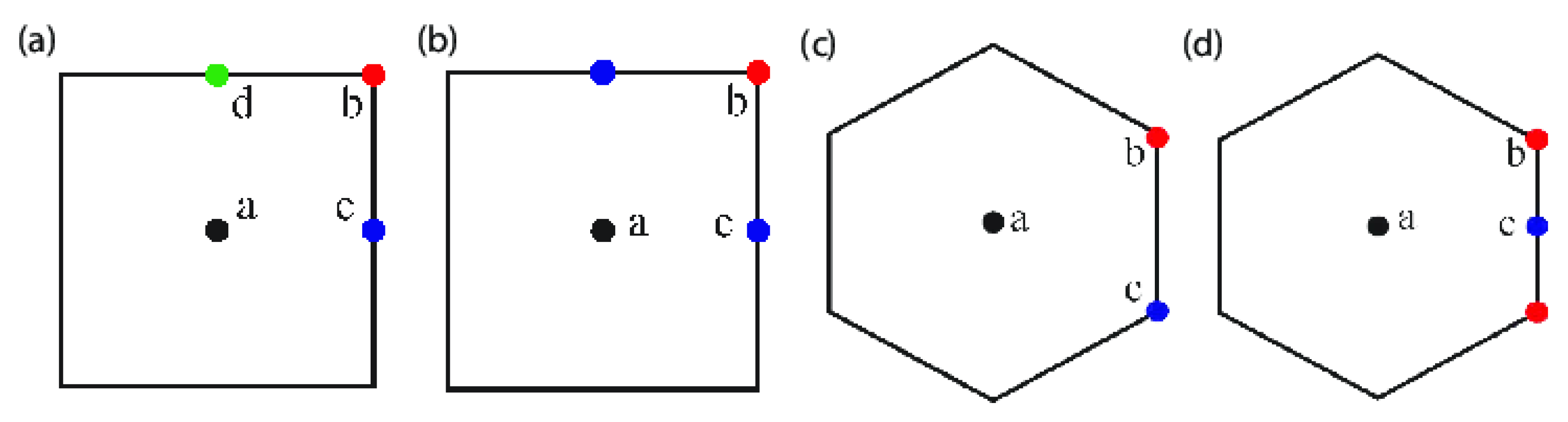
Features must be extracted from a Wyckoff position for the crystal to be used for CNN training and validation. Crystals are classified from the testers in various Wyckoff positions, as depicted in Figure 1.

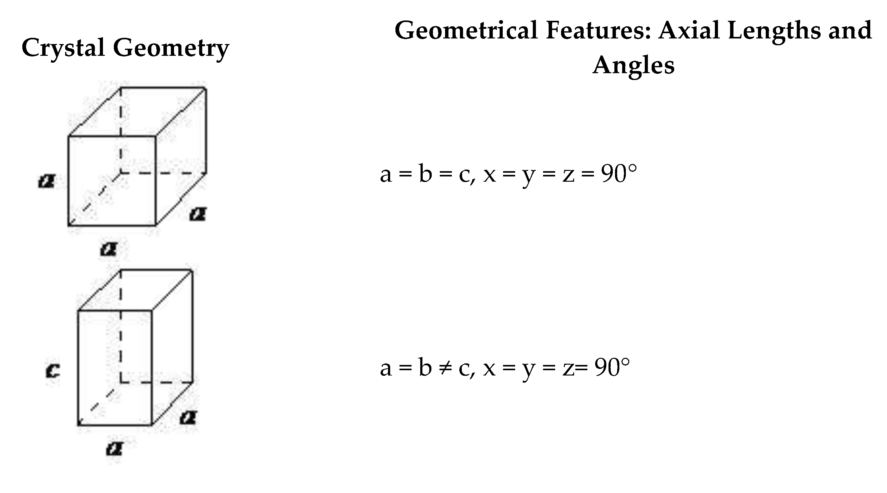
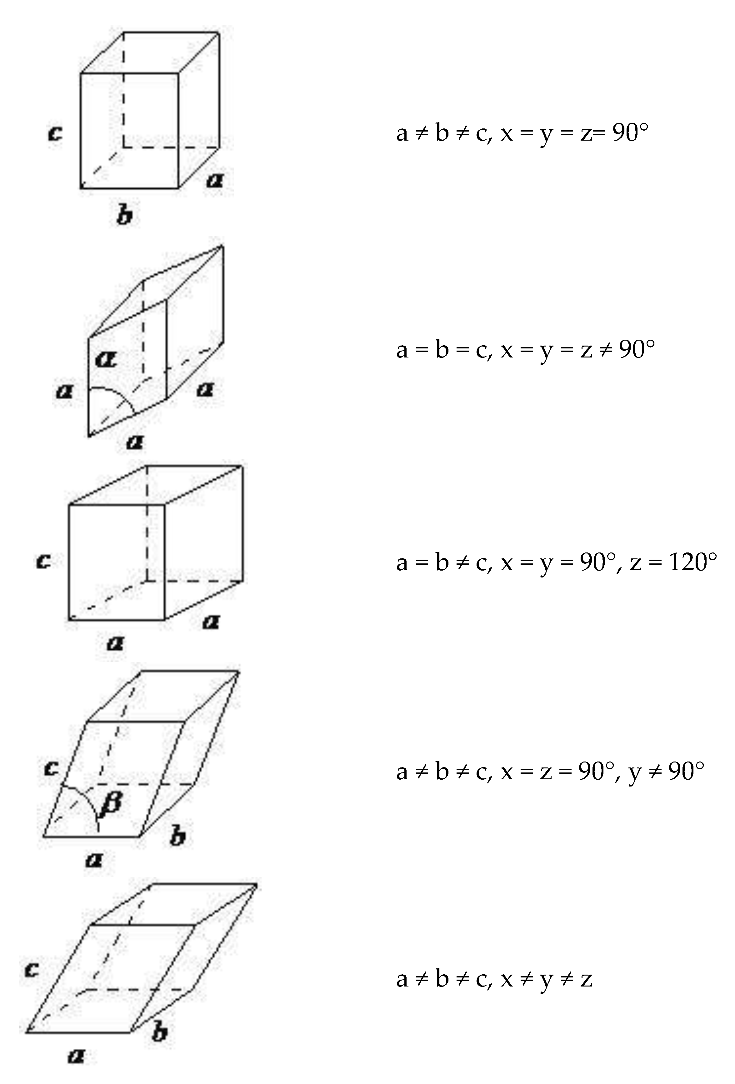
The crystals are characterized with a method where multiple sites of the crystals are situated. It is projected that the crystal overlay and their displacements are uniformly distributed. The crystals are Wyckoff-sited in the cubic space to form the volume of the crystals (S = a × b × c). There are multiple parameters in the crystal (the shape parameters, namely the angles in the three dimensions x,y,z of the structure), as depicted in Figure 2. The unit cell segment volume (V) is computed from the lattice lengths (a,b,c) and angles (x,y,z). Given that the cell sides are denoted as vectors, the volume V is the scalar product of the three vectors. The volume is computed as follows:

$$V=a\times b\times c\sqrt{1+2\cos x\cos y\cos z-{cos}^{2}x-{cos}^{2}y-{cos}^{2}z}$$

The parameters are the segment volume (V); the threshold (€), which crystallographically describes the distinguishable threshold between different crystals; the average distance between atoms of the crystals (w_Avg); and the distance variance (σ²), which is the deviation of the predicted distance w_Avg from the ground truth from the labelled crystals in the dataset.

The restorations have a w_Avg of 1.2 mm (unit), σ² is equal to 0.7 mm, and € is equal to 0.13, which are all static values. The loci are unfixed with variable values 0.19 up to 0.35 with a step of 0.2.

Once the parameters of the built crystals are calculated, the crystals in the lattice of the arrangement use the concentration (Conc) gradient ($\frac{\partial Conc}{\partial t}$). This is organized by the crystal distribution rules [33], which are formulated as follows:

$$\frac{\partial Conc}{\partial t}=\nabla \left(S_b-\nabla Conc\right)$$

(1)

where S_b is the Wyckoff crystal structure–property value. The concentration in the space is denoted by Conc_out at threshold € ≤ 0.13. The three dimensions (x, y, and z), where the borderline settings for the conforming domains are depicted as follows:

$$Conc={Conc}_{in}, x=0 and >0$$

(2)

$$\frac{\partial Conc}{\partial x}={Conc}_{out}, x=S_{\mathit{bx}} and €\le 0.13,$$

$$\frac{\partial Conc}{\partial y}=0, y=0 or S_{\mathit{by}} and €\le 0.13,$$

$$\frac{\partial Conc}{\partial z}=0, z=0 or S_{\mathit{bz}} and €\le 0.13$$

The crystal’s structure–property PSP method calculates the real structure–property value in the learning stage of the deep learning model. The PSP method is precise in classifying the crystal’s structure–property [35].

The structure–property formulas use the time series technique, in which the definite structure–property value of complex substance is realized. The PSP algorithm is shown in Figure 3.

The Wyckoff function to calculate the PSP parameters P_i (i = 1 to n) is defined as follows:

$$P_i\left(Conc+S_{i}t,T+t\right)-P_i\left(Conc,T\right)=\frac{1}{r}\left[P_i\left(Conc,T\right)-P_i^{\mathit{equil}}\left(Conc,T\right)\right]$$

(3)

where P_i is the crystal distribution parameter, C is the location, S is the structure vector, t is the time step, $P_i^{\mathit{equil}}$ is the equilibrium point, and T is the current relaxation period.

D is the Wyckoff function of the crystal structure–property value, which is defined as follows:

$$D=\frac{3S_d}{{Conc}^{2}t}+\left(\frac{1}{2}\right)$$

(4)

To eliminate computational errors in the experiment, the reduction period is given a value so that it is proven to be stable. Non-stable patterns are used at the input and intermediate computations for fixed attentions. These patterns are performed on the three axes due to the accuracy in the border shape width [37–42]. The manner in which the PSP determines the unbalanced crystal structure–property data in order to realize the steady-state condition is depicted as follows:

$${Conc}_{\mathit{steady}\mathit{state}}=\sqrt{{\sum }_{x,y,z}{\left({Conc}_{x,y,z}^{t+\frac{1}{2}}-{Conc}_{x,y,z}^t\right)}^2/{\sum }_{x,y,z}{\left({Conc}_{x,y,z}^{t+\frac{1}{2}}\right)}^2<€}$$

(5)

where ${Conc}_{x,y,z}^{t+\frac{1}{2}}$ and ${Conc}_{x,y,z}^t$ are defined in the period t to $t+\frac{1}{2}$. The structure–property, the concentration (Conc), and the crystals’ weight Wt at each axis can be calculated as follows:

$$Conc=\sum _i{S}_i$$

(6)

$$Wt=\left({Wt}_x,{Wt}_y,{Wt}_z\right)\sum _i{\left(S_i\right)}^{\frac{t-0.5}{\tau }}$$

(7)

After computing (Conc) and (Wt) at each axis, the real structure–property value of the crystal structure is standardized by dividing the value across the structure–property axis.

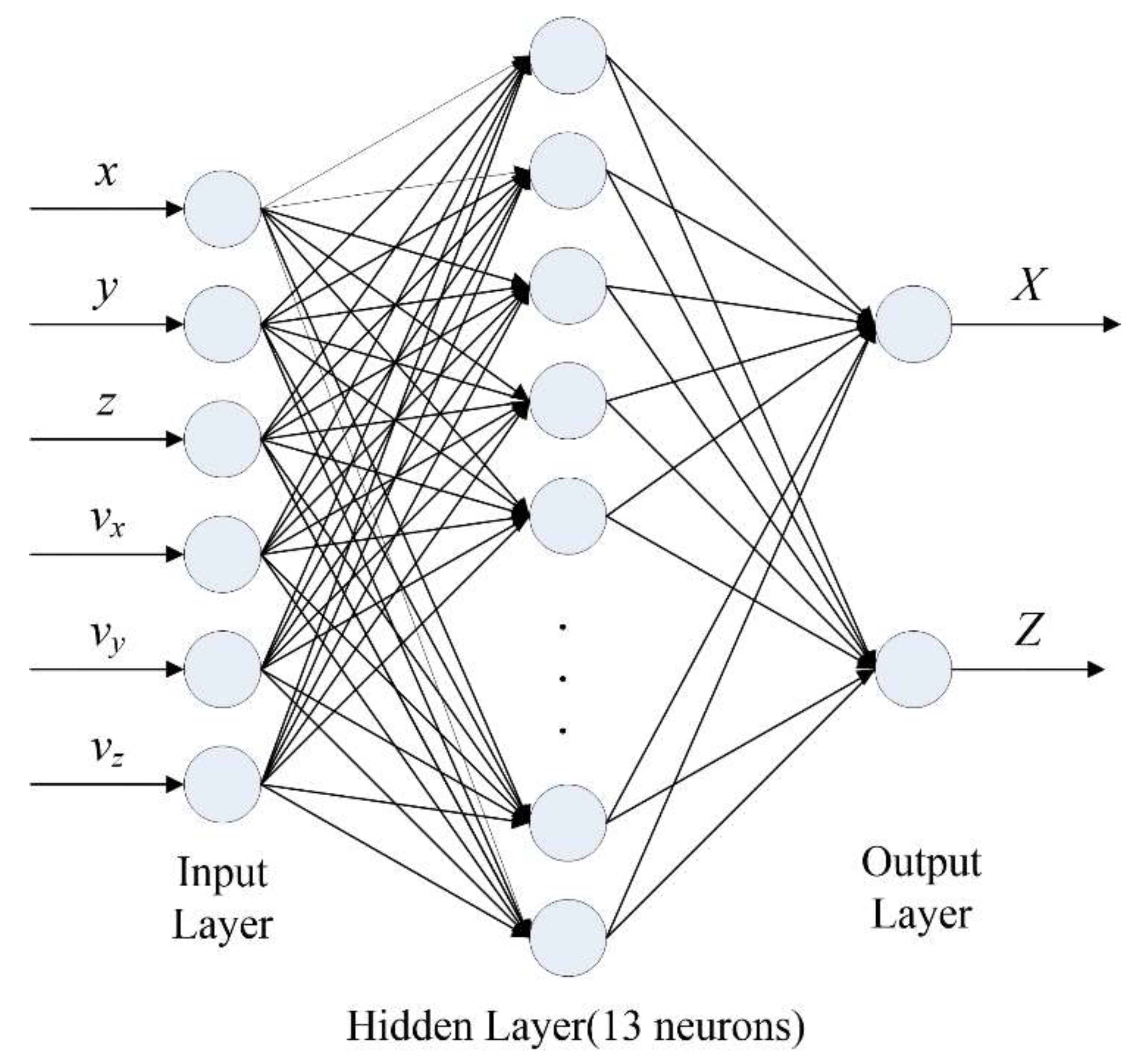
The proposed CNN uses an input layer that is fed with input blocks to learn the convolutional layers from these blocks. The ReLu Wyckoff function extracts the key parameters of those blocks. The average pooling layer will calculate the mean value via the vector produced by the pooling layer to lessen the CPU time load and to extract the significant parameters. The selected layer escapes the overfitting problem by erasing part of the produced pooled output. The pooled output and the dense layers will declare the last classification choice. In this article, the input is fed into the dense layers which select key parameters and build the representative vectors. The average parameter values are sampled by the average pooling of double layers. The characterized parameter vectors are fed to the ReLU layer to represent nonlinear features. The dense layers will incorporate the data and classify it.

2.1. The Augmentation CNN Training Phase

The proposed CNN model has an input initial layer that utilizes input partitions and fed the input into the dense layers. The dense layers extract the key parameters of each convolution block. The average pooling then calculates the average from the feature vector partition between the pooling filter to reduce the CPU time and extract the significant features. Dropout functions are used to evade overfitting by eliminating random portions of the output. The dense layers select the ultimate predicted class. In our paper, the input objects are fed into the neural layers which select the parameters and compute the feature vectors. The average feature vectors are combined by the average pooling Wyckoff function. The selected feature vectors are fed into the ReLU to add nonlinear values. The dense layers will summarize the vectors and fed it to the classifier.

2.2. The Augmentation of the CNN Learning Stage

The learning stage of deep learning techniques needs a large training dataset. Long impractical training times are also required. To solve this issue, a particular crystal will be altered via a data augmentation algorithm. In our model, large vacancies and their selected parameters are divided into lower dimension crystal using the sliding box three-dimensional algorithm (SBT). An (8 × 8 × 8) sliding box slides across the original data to increase the number of data items. During the box sliding, symbolic structures are chosen to stop the SBT from choosing equivalent blocks. The real structure–property functions of the lesser volume crystals can be calculated with the approved crystal weight through crystal structure–property actions. The foundations for using the sliding augmentation model are described. At the final phase, we divide all the 24 primary lattice crystals with sizes 0.23 and 0.41 and units of (256 × 256 × 256) into sub-structures with dimensions of (128 × 128 × 128). The dimensions of the computed sub-structures have sizes which range from 0.35 to 0.51. The features of the computed sub-structures (128 × 128 × 128) are altered from the primary crystal, because computing lower dimension sub-structures produces randomness. The primary crystals contain lattices with an unsystematic shape and the generated sub-structure has an unsystematic shape. The course of dividing the primary large crystals into lower dimension sub-structures will produce a diverse crystal weight distribution. Their real structure–property functions are calculated by their crystal weight values. This process can reduce the time generating ample crystals and the time using the chemistry labs. The produced 16,000 sub-structures and their calculated real structure–property functions are utilized in the training phase.

2.3. The Proposed CNN Neural Model

The crystal is a combination of crystal diffraction images captured from frontal views. The three-dimensional relations are used by the dense layers. A deep learning model can diminish the time-consuming challenge and permit the computation with a structure instead of a construct.

The data pattern and its real structure–property value are fed as input.

$${Sub}_i=\{x,y,z,G\left(x,y,z\right)\}\mathit{where} i=1 to N$$

(8)

where x,y,z are the real axis and each value is from 1 to 128, and N is equal to 16,000.

$$G\left(x,y,z\right)=g\{\begin{array}{c}g\ge 1\left(\mathit{solid}\right)\\ g=0\left(\mathit{hole}\right)\end{array}$$

(9)

The real structure–property value is calculated by the PSP. Dimensions of 0.42 and 0.51 are utilized for training. Henceforward, a down-sized training dataset with 8000 items are fed into the input layer. Other data (4000) with lattice of sizes 0.31 to 0.71 are utilized in classification [21].

3. Experimental Results

In this section, we study the precision of the proposed PSP model, where hyper-parameters are selected.

3.1. Datasets

This research proposes a deep learning technique on the dataset of crystal structures utilizing Wyckoff positions. The dataset is a public dataset found at [21]. The datasets are composed of high-resolution crystal lattice structures images taken as diffraction images. We utilized two datasets: the first one is composed of 8000 labelled samples of sizes larger than 0.71 mm, while the second dataset is composed of 4000 labelled samples with lattice of sizes 0.31 mm to 0.71 mm to be utilized in classification [21].

The two datasets are distributed, as depicted in

Table 2. The distribution of the datasets.

Crystal Structure	First Dataset	Second Dataset
Perovskite	1300	950
Layered perovskite	1200	800
Spinel	1500	860
Fluorite	1300	802
Halite	1250	870
Ilmenite	1450	718

. The datasets are partitioned as 70% for training 15% for validation and 15% for testing.

Some Wyckoff positions with site symmetry and their coordinates are depicted in

Table 3. Wyckoff positions with site symmetry and their coordinates.

Wyckoff Position	Site Symmetry	Coordinate
32p	1	x,y,z
16o	.m.	x,y,0
16n	m..	x,0,z
16m	2..	0,y,z
16l	.2.	x,$\frac{1}{4},\frac{1}{4}$
16k	..2	$\frac{1}{4},y,\frac{1}{4}$
16j	mm2	$\frac{1}{4},y,\frac{1}{4}$
8i	m2m	0,0,z
8h	2mm	0,y,0
8g	222	x,0,0
8e	..2/m	$\frac{1}{4},\frac{1}{4},\frac{1}{4}$
8d	.2/m.	$\frac{1}{4},\frac{1}{4},0$
8c	2/m..	$\frac{1}{4},0,\frac{1}{4}$
4b	mmm	$0,\frac{1}{4},\frac{1}{4}$
4a	mmm	0,0,0

.

3.2. Extraction of the Hyper-Parameters

The hyper-parameters are the count of dense layers D_L, the seed size Seed_s, the count of nodes in each dense layer N Node_D, and the ReLU functions Re_act. These factors are computed prior to the training phase. The hyper-parameters enhance the model’s accuracy. The hyper-parameters are extracted by reducing the mean square error (MSE) from the m input substructures and are calculated as follows:

$$MSE=\frac{1}{m}\sum _{k=1}^m|\left(S_{Conc}{\left(eff\right)}^{ADA}-S_{Conc}{\left(eff\right)}^{CNN}\right)|$$

(10)

When the MSE Wyckoff functions converge, the hyper-parameters are deliberated as acceptably learned. Then, the PSP concentration prediction S_Conc(eff) will be calculated to be used as an accuracy metric for extracting the hyper-parameters.

Table 4. Total error of the CNN models with hyper-parameters.

Number of CNN Convolutional Layers	Dropout Values
	0.5	0.7	0.9
	Total Error Value
12	4.5	–	–
16	1.5	0.8	–
20	0.4	0.3	0.1

shows the mean square error of the predicted results and the actual values. The total square error T is calculated as follows:

$$T=\frac{\left|\left(S_{Conc}{\left(eff\right)}^{ADA}-S_{Conc}{\left(eff\right)}^{CNN}\right)\right|}{S_{Conc}{\left(eff\right)}^{CNN}}$$

(11)

The training curve, as shown from Table 2, proves that:

• Growing the dropout value enhances the precision value.
• Organizing 20 CNNs and higher dropout values attains higher precision and less error.
• The proposed model attains a low 0.1 total error in the testing phase.

The learning cross-entropy value will quickly converge and narrowly converge at 500 epochs. The cross-entropy value fluctuates in the procedure and lessens to 0.05 after 1400 epochs. The testing cross-entropy value will congregate, proving that the introduced method will stabilize, as displayed in Figure 4.

Figure 5 depicts the training and validation loss values versus the mean square error of the proposed classification model. The results are calculated by the PSP and averaged over 100 cases, which are then divided into sub-structures. Each sub-structure depicts the probability of the corresponding experiment. The probability values define the percentage of the data accommodating various square error values.

After model testing and validation, the hyper-parameters are computed. The structure of the CNN model is displayed in

Table 5. CNN model layers and hyper-parameters.

Layer Number	Layer	Filter Size	Activation
1	Input	56 × 56 × 56	–
2	Dense layers	36/5 × 5 × 3	–
3	Average pooling	5 × 5 × 5	ReLU
4	Dense Layers (second block)	60/5 × 5 × 3	–
5	Pooling	2 × 2 × 2 (max)	ReLU
6	Dropout layer	0.5–0.7–0.9	–
8	Regulation	46	ReLU
9	Dense layers (third block)	90/5 × 5 × 3	–
10	Dropout	0.5	–
11	Classifier		Softmax
12	Output		–

.

The correctness of the CNN is confirmed by comparing the ground truth structure–property value in the Softmax classifier of the CNN and the PSP structure that computes the real structure–property values for the testing data with lattice of sizes 0.32 to 0.71, as predicted by the model, the PSP, and the results in [40].

To study the accuracy of the proposed model, several metrics are employed, which demonstrate the model’s efficiency in classifying atom diffusion from the diffraction images. The performance metrics are recall, f1-score, precision, and accuracy, as depicted in

Table 6. Classification report of our model with augmentation learning.

	Our Model with Augmentation Learning
Predicted Crystal Structure	Precision	Recall	F2-Score
Perovskite	0.97	0.99	0.96
Layered perovskite	0.96	0.96	0.96
Spinel	0.96	0.96	0.97
Fluorite	0.97	0.92	0.96
Halite	0.98	0.94	0.97
Ilmenite	0.96	0.95	0.95

.

$$\mathit{Precision}=\frac{TP}{TP+FP}$$

(12)

$$\mathit{Recall}=\frac{TP}{TP+FN}$$

(13)

$$\mathit{Accuracy}=\frac{TP+TN}{TP+TN+FP+FN}$$

(14)

$$F2-\mathit{Score}=\frac{2\times \mathit{Recall}\times \mathit{Precision}}{\mathit{Recall}+\mathit{precision}}$$

(15)

The confusion matrix of predicting structure–property from diffraction images in

Table 7. Confusion matrix for the proposed PSP.

Crystal Structure	Perovskite	Layered Perovskite	Spinel	Fluorite	Halite	Ilmenite	Total Cases
Perovskite	3900	20	50	30	0	0	4000
Layered perovskite	10	3940	20	10	0	0	4000
Spinel	15	5	3450	30	0	0	3500
Fluorite	0	0	26	4470	0	4	4500
Halite	0	5	10	30	4150	5	4200
Ilmenite	10	4	6	10	1	3669	3700

depicts the ground truth vertically and the predicted structure–property horizontally from the generated images of 16,000 sub-structures.

In this paper,

Table 8. Performance comparison of the proposed model versus state-of-the-art models.

Reference	Model	Average Accuracy (%)	Average Training Time (Hours)	Average Classification Time (Seconds)
	The proposed PSP model	98.5%	11.6	75.3
[18]	Structure–property in crystals with different lattice distribution classifications	91.5%	18.1	313.1
[19]	Structure–property in crystals with different lattice distribution classifications	93.5% with a higher CPU time	22.9	619.9
[20]	Structure–property in crystals with different lattice distribution gradings	93.67%	17.3	90.3
[21]	Structure–property in crystals with different lattice distribution classifications	92.2%	16.3	250.4
[22]	Diffraction images structure–property in crystals with different lattice distribution gradings	92.8%	24.2	412.5
[23]	Prediction of structure–property in crystals with different lattice distributions at a high speed	91.3%,	17.2	515.7

compares the training time between our model and other state-of-the-art models, contrasting the deep learning model and how transfer learning can affect the training time complexity. It is also significant to track the trade-off between the CPU time and the attained accuracy.

4. Conclusions

In this article, we characterized a framework to precisely predict the structure–property value of a crystal by using a deep learning technique. The crystals of the defect structure are generated using distribution functions. The actual structure–property value of the structure is realized by a vacant-defect value by simulating the proposed PSP model. The cubic data, computed from the processes, are used as an input into the CNN network for training, validation, and testing stages. The experiment’s results prove that these crystals are very useful in the convergence of the training learning curve. Although lattice of sizes between 0.40 and 0.50 are used in the training phase, the CNN model established a high learning capacity and realized the lower mean square errors of ranges equal 0.018% to 1.97% in the testing stage that involved lattice sizes of 0.31 and 0.71. When the lattice size reached 0.6, the PSP realized a smaller CPU training time equal to 11.16 h. Both the CPU training time and classification time are much lower as compared to other models. This proved that our proposed deep leaning model is a powerful technology that can be employed to predict the structure–property values of composite crystal structures.

References

1. Ji, S.; Xu, W.; Yang, M.; Yu, K. Cube’ convolutional neural networks for human action recognition. IEEE Trans. Pattern Anal. Mach. Intell. 2021, 35, 221–231. [Google Scholar] [CrossRef] [PubMed] [Green Version]
2. Hussain, M.; Tian, E.; Cao, T.-F.; Tao, W.-Q. Pore-scale modeling of actual structure–property coefficient of building crystals. Int. J. Heat Weight. Transf. 2021, 90, 1266–1274. [Google Scholar] [CrossRef]
3. Zamel, N.; Li, X. Actual transport properties for polymer electrolyte membrane fuel cells-With a focus on the gas structure–property layer. Prog. Energy Combust Sci. 2013, 39, 111–146. [Google Scholar] [CrossRef]
4. Wang, H.; Qu, Z.G.; Zhou, L. Coupled GCMC and LBM simulation method for visualizations of CO2/CH4 gas separation through Cu-BTC membranes. J. Membr. Sci. 2018, 550, 448–461. [Google Scholar] [CrossRef]
5. Qu, Z.G.; Yin, Y.; Wang, H.; Zhang, J.F. Pore-scale investigation on coupled structure–property mechanisms of free and adsorbed gases in nanoorganic matter. Fuel 2020, 260, 112–130. [Google Scholar] [CrossRef]
6. Wang, H.; Chen, L.; Qu, Z.; Yin, Y.; Kang, Q.; Yu, B.; Tao, W.Q. Modeling of multi-scale transport phenomena in shale gas production-A critical review. Appl. Energy 2020, 262, 114575. [Google Scholar] [CrossRef]
7. Roque-Malherbe, R.M.A. Adsorption and Structure–Property in Nanocrystal Structures; CRC Press: Boca Raton, FL, USA, 2007. [Google Scholar]
8. Kärger, J.; Valiullin, R. Weight transfer in mesocrystal structures: The benefit of microscopic structure–property measurement. Chem. Soc. Rev. 2013, 42, 4172. [Google Scholar] [CrossRef]
9. Falk, K.; Coasne, B.; Pellenq, R.; Ulm, F.-J.; Bocquet, L. Subcontinuum weight transport of condensed hydrocarbons in nanomedia. Nat. Commun. 2020, 6, 6949. [Google Scholar] [CrossRef] [Green Version]
10. Ryan, E.M.; Mukherjee, P.P. Mesoscale modeling in electrochemical devices—A critical perspective. Prog. Energy Combust. Sci. 2019, 71, 118–142. [Google Scholar] [CrossRef]
11. Ryan, E.M.; Mukherjee, P.P. Deconstructing electrode pore network to learn transport distortion. Phys. Fluids 2019, 31, 122005. [Google Scholar]
12. Bulat, F.A.; Toro-Labbe, A.; Brinck, T.; Murray, J.S.; Politzer, P. Quantitative analysis of molecular surfaces: Areas, volumes, electrostatic potentials and average local ionization energies. J. Mol. Model. 2010, 16, 1679–1691. [Google Scholar] [CrossRef]
13. Alvarez-Ramírez, J.; Nieves-Mendoza, S.; González-Trejo, J. Calculation of the actual diffusivity of heterogeneous media using the lattice-Boltzmann method. Phys. Rev. E. 1996, 53, 2298–2303. [Google Scholar] [CrossRef]
14. Wu, H.; Fang, W.Z.; Kang, Q.; Tao, W.Q.; Qiao, R. Predicting Effective Diffusivity of Porous Media from Images by Deep Learning. Sci. Rep. 2019, 9, 20387. [Google Scholar] [CrossRef] [Green Version]
15. Macrae, C.F.; Sovago, I.; Cottrell, S.J.; Galek, P.T.A.; McCabe, P.; Pidcock, E.; Platings, M.; Shields, G.P.; Stevens, J.S.; Towler, M.; et al. Mercury 4.0: From visualization to analysis, design and prediction. J. Appl. Cryst. 2020, 53, 226–235. [Google Scholar] [CrossRef] [Green Version]
16. Mezedur, M.M.; Kaviany, M.; Moore, W. Effect of pore structure, randomness and size on actual weight diffusivity. AlChE J. 2002, 48, 15–24. [Google Scholar] [CrossRef] [Green Version]
17. Chen, L.; Zhang, L.; Kang, Q.; Viswanathan, H.S.; Yao, J.; Tao, W. Nanoscale simulation of shale transport properties using the lattice Boltzmann method: Permeability and diffusivity. Sci. Rep. 2020, 5, 8089. [Google Scholar] [CrossRef] [Green Version]
18. Chen, L.; Kang, Q.; Dai, Z.; Viswanathan, H.S.; Tao, W. Permeability classification of shale matrix recharacterized using the elementary building block model. Fuel 2021, 160, 346–356. [Google Scholar] [CrossRef]
19. Chen, L.; Fang, W.; Kang, Q.; Hyman, J.D.H.; Viswanathan, H.S.; Tao, W.Q. Generalized lattice Boltzmann model for flow through tight porous media with Klinkenbergs effect. Phys. Rev. E 2022, 91, 033004. [Google Scholar] [CrossRef] [Green Version]
20. Lunati, I.; Lee, S. A dual-tube model for gas dynamics in fractured nanoporous shale formations. J. Fluid Mech. 2014, 757, 943–971. [Google Scholar] [CrossRef] [Green Version]
21. Li, C.; Nilson, T.; Cao, L.; Mueller, T. Predicting activation energies for vacancy-mediated structure–property in alloys using a transition-state cluster expansion. Phys. Rev. Mater. 2021, 5, 013803. Available online: https://spglib.github.io/spglib/dataset.html (accessed on 1 January 2022). [CrossRef]
22. Yang, Z.; Yabansu, Y.C.; Al-Bahrani, R.; Liao, W.K.; Choudhary, A.N.; Kalidindi, S.R.; Agrawal, A. Deep learning approaches for mining structure-property linkages in high contrast composites from simulation datasets. Comput. Cryst. Sci. 2018, 151, 278–287. [Google Scholar] [CrossRef]
23. Cecen, A.; Dai, H.; Yabansu, Y.C.; Kalidindi, S.R.; Song, L. Crystal structure-property linkages using three-dimensional convolutional neural networks. Acta Cryst. 2018, 146, 76–84. [Google Scholar]
24. Krizhevsky, A.; Sutskever, I.; Hinton, G.E. Advances in neural information processing systems. In Proceedings of the 30th Annual Conference on Neural Information Processing Systems 2016, Barcelona, Spain, 5–10 December 2016; pp. 1097–1105. [Google Scholar]
25. Cireşan, D.; Meier, U.; Schmidhuber, J. Multi-column deep neural networks for image classification. arXiv 2021, arXiv:1202.2745. [Google Scholar]
26. LeCun, Y.; Bottou, L.; Bengio, Y.; Haffner, P. Gradient-based learning applied to document recognition. Proc. IEEE 1998, 86, 2278–2324. [Google Scholar] [CrossRef] [Green Version]
27. Wu, J.; Yin, X.; Xiao, H. Seeing permeability from images: Fast classification with convolutional neural networks. Sci. Bull. 2020, 63, 1215–1222. [Google Scholar] [CrossRef] [Green Version]
28. Cang, R.; Li, H.; Yao, H.; Jiao, Y.; Ren, Y. Improving direct physical properties classification of heterogeneous crystals from imaging data via convolutional neural network and a morphology-aware generative model. Comput. Cryst. Sci. 2021, 150, 212–221. [Google Scholar]
29. Srisutthiyakorn, N. Deep-learning methods for predicting permeability from flattened/binary-segmented images. SEG Tech. Program Expand. Abstr. 2019, 2016, 3042–3046. [Google Scholar]
30. Wang, M.; Wang, J.; Pan, N.; Chen, S. Mesoscopic predictions of the actual thermal conductivity for microscale random porous media. Phys. Rev. E 2020, 75, 036702. [Google Scholar] [CrossRef] [Green Version]
31. Fang, W.-Z.; Gou, J.-J.; Chen, L.; Tao, W.-Q. A multi-block lattice Boltzmann method for the thermal contact resistance at the interface of two solids. Appl. Therm. Eng. 2021, 138, 122–132. [Google Scholar] [CrossRef]
32. LeCun, Y.; Bengio, Y.; Hinton, G. Deep learning. Nature 2020, 521, 436. [Google Scholar] [CrossRef]
33. LeCun, Y.; Bengio, Y. Convolutional networks for images, speech, and time series. In The Handbook of Brain Theory and Neural Networks; ICM: Winnipeg, MB, Canada, 1995; Volume 3361. [Google Scholar]
34. Dollár, P.; Appel, R.; Belongie, S.; Perona, P. Fast feature pyramids for object detection. IEEE Trans. Pattern Anal. Mach. Intell. 2020, 36, 1532–1545. [Google Scholar] [CrossRef] [PubMed] [Green Version]
35. Ramachandran, P.; Zoph, B.; Le, Q.V. Searching for activation functions. arXiv 2021, arXiv:1710.05941. [Google Scholar]
36. Aghdam, H.H.; Heravi, E.J. Guide to Convolutional Neural Networks; Springer: New York, NY, USA, 2019; Volume 10, pp. 973–978. [Google Scholar]
37. He, K.; Zhang, X.; Ren, S.; Sun, J. European Conference on Calculator Vision; Springer: Berlin/Heidelberg, Germany, 2022; pp. 630–645. [Google Scholar]
38. Zhang, H. The band structures of three-dimensional nonlinear plasma photonic crystals. AIP Adv. 2018, 8, 015304. [Google Scholar] [CrossRef]
Figure 1. Wyckoff sites in unit cells of (a) C2; (b) C4; (c) C3; (d) C6 two-dimensional Bravais lattices (similar colors specify equivalent Wyckoff positions). Wyckoff positions are symbolized by a, b, c, and d.
Crystals 12 01460 g001
Figure 2. Geometrical features: axial lengths and angles of crystal structures.
Crystals 12 01460 g002aCrystals 12 01460 g002b
Figure 3. The deep learning PSP and classification.
Crystals 12 01460 g003
Figure 4. The cross-entropy value in the training and validation operations.
Crystals 12 01460 g004
Figure 5. The training and validation loss values versus the mean square error.
Crystals 12 01460 g005