Predicting Perovskite Performance with Multiple Machine-Learning Algorithms

Abstract

Perovskites have attracted increasing attention because of their excellent physical and chemical properties in various fields, exhibiting a universal formula of ABO₃ with matching compatible sizes of A-site and B-site cations. In this work, four different prediction models of machine learning algorithms, including support vector regression based on radial basis kernel function (SVM-RBF), ridge regression (RR), random forest (RF), and back propagation neural network (BPNN), are established to predict the formation energy, thermodynamic stability, crystal volume, and oxygen vacancy formation energy of perovskite materials. Combined with the fitting diagrams of the predicted values and DFT calculated values, the results show that SVM-RBF has a smaller bias in predicting the crystal volume. RR has a smaller bias in predicting the thermodynamic stability. RF has a smaller bias in predicting the formation energy, crystal volume, and thermodynamic stability. BPNN has a smaller bias in predicting the formation energy, thermodynamic stability, crystal volume, and oxygen vacancy formation energy. Obviously, different machine learning algorithms exhibit different sensitivity to data sample distribution, indicating that we should select different algorithms to predict different performance parameters of perovskite materials.

1. Introduction

With the progress of science and technology as well as the development of social economy, people are very active in the research on the development and utilization of various energy resources [1,2,3,4,5,6]. In recent years, ABO₃ perovskite composite oxides have attracted great interest [3,4,7,8,9,10,11,12,13,14,15]. Research has focused on the development of new perovskite materials to improve activity, selectivity, and stability, as well as the development of advanced manufacturing techniques to reduce their cost while ensuring their reliability, safety, and reproducibility [14,15,16]. In ABO₃ perovskite oxides, the A site is the rare earth or alkaline earth metal ions, which usually stabilize the structure, while the B site is occupied by the smaller transition metal ions [17]. Through partial substitution of A and B sites, multi-component perovskite compounds can be combined [16]. When A or B sites are partially replaced by other metal ions, anion defects or B sites at different valences can be formed. This improves the properties of the compounds but does not fundamentally change the crystal structure [17]. This kind of composite oxide has gas sensitivity, oxidation catalytic property, conductivity, oxygen permeability, and other properties. In addition, its structure and performance are closely related to the composition of the system [17]. Perovskite-type oxides can form compounds through partial doping of metal ions at A and B sites on the basis of maintaining stable crystal structure, as well as controlling the elements and valence states so that the performance of perovskite materials present rich diversity [18,19,20].

The research in the field of materials is generally based on the successful preparation of experimental samples. The various properties of samples are measured to understand the various physical properties, and the materials are analyzed and classified through different performance parameters [21]. The traditional material experimental process has a strong dependence on the samples. A lot of repetitive work during the experiment process leads to long development times. With the continuous development of computer science, many methods, such as first-principles calculation, phase field simulation, and finite element analysis, have emerged to investigate the structure and performance of materials, but they are often large and costly. These are the major factors limiting the development and transformation of materials [22,23,24].

With the fast development of artificial intelligence, many researchers have applied machine learning methods to accelerate material sciences [25,26]. Due to its strong data processing capacity and relatively low research threshold, machine learning can effectively reduce the cost of human and material resources in industrial development and shorten the research and development cycle [27]. By replacing or cooperating with traditional experiments and computational simulation, it can analyze material structure and predict material properties more quickly and accurately, so as to develop new functional materials more effectively [28,29]. Selecting different machine learning methods to predict material performance parameters from existing large data sets can effectively improve the prediction accuracy of material performance, so as to select materials with reasonable performance for experimental research [21]. Using existing data to predict the performance parameters can not only expand the space of material data but also provide guidance for material experiments and applications. Different machine learning algorithms have different sensitivities to material data in different ranges of data sets, so it is necessary to make a feature selection on specific material data samples to evaluate algorithm by performance evaluation [30,31,32].

The perovskite data set calculated based on the first principles and density functional theory by Antoine et al. was selected as the training samples [33]. Weike et al. showed that deep neural networks utilizing just two descriptors (the Pauling electronegativity and ionic radii) can predict the DFT formation energies of C₃A₂D₃O₁₂ garnets and ABO₃ perovskites with low mean absolute errors (MAEs) [34]. Wei et al. developed machine learning models to predict the thermodynamic phase stability of perovskite oxides using a dataset of more than 1900 DFT-calculated perovskite. 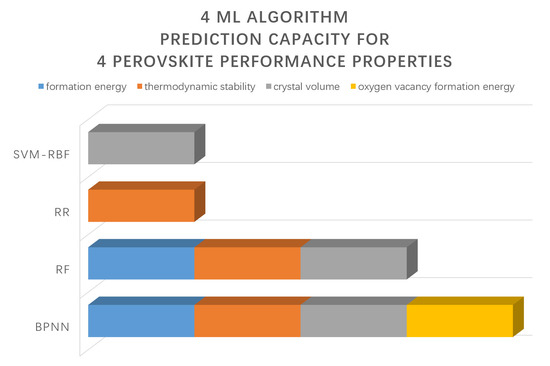The results showed that that error is within the range of errors in DFT formation energies relative to elemental reference states when compared to experiments and, therefore, may be considered sufficiently accurate to use in place of full DFT calculations [35]. Using different machine learning algorithms, the formation energy, thermodynamic stability, crystal volume, and oxygen vacancy formation energy of perovskite materials were predicted [36,37].

As shown in Figure 1,

Step 1: The original dataset (0) was divided (1) into training dataset (2) and test dataset (5).

Step 2: A different algorithm (3) was trained based on the training dataset (2) into different models (4).

Step 3: Trained models (4) were used to predict test dataset (6).

Step 4: Performance evaluations (7) were obtained by calculation of predicted value and true value.

Four kinds of machine learning algorithms were used to establish the multi-algorithm prediction model for the multi-performance parameters of perovskite materials, and the prediction accuracy of the model was compared and evaluated. The experimental results have important reference value and practical significance for the further study of machine learning methods in the prediction of perovskite material properties and the discovery of new perovskite materials.

2. Principles and Methods

2.1. Regression Prediction of Support Vector Machines

According to the limited sample information, SVM seeks the best compromise between the complexity of the model and the learning ability to obtain the best generalization ability based on statistical learning theory [38,39,40]. SVM has many unique advantages in solving small sample, nonlinear, and high-dimensional pattern recognition. Its basic idea is to map the data x to the high-dimensional feature space F through a nonlinear mapping ϕ and make linear regression in this space.

Assume a sample set $\{\left(x_i,y_i\right){\}}_i^N,$ in which the input data are $x_i\in R^n, y_i\in R^n,$ and the optimal linear model function constructed in high dimensional space is:

$$f\left(x\right)={\omega }^T\varphi \left(x\right)+b$$

(1)

where ω and b are weight and bias item, respectively. Thus, the linear regression in the high dimensional feature space corresponds to the nonlinear regression in the low dimensional input space.

When using SVM to solve regression problems, we need to use the appropriate kernel function instead of inner product according to the characteristics of solving problems, so as to implicitly transform the inner product operation of high-dimensional feature space into the kernel function operation of low dimensional original space. This skillfully solves the “dimension disaster” caused by calculation in high-dimensional feature space [36]. The commonly used kernel functions are RBF, linear, etc. [39]. In addition, SVM introduces a parameter ε insensitive loss function and uses the loss function to complete the linear regression in the high-dimensional feature space, while the complexity of the model is reduced by minimizing ${\left|\right|\omega \left|\right|}^2$. Finally, the objective function of SVM is as follows:

$$\underset{\omega ,b,\xi ,{\xi }^{\prime }}{\mathit{min}}J\left(\omega ,\xi ,{\xi }^{\prime }\right)=\frac{1}{2}{\omega }^T\omega +C{\displaystyle \sum }_{i=1}^n\left(\xi +{\xi }^{\prime }\right)$$

(2)

Here, we introduce a nonnegative relaxation variable ξ and ξ’, and C is a regularization parameter to control the penalty for the samples that exceed the error.

2.2. Random Forest

The random forest (RF) regression algorithm is a combination algorithm based on the decision tree classifier [36,41,42,43,44]. It uses the bootstrap re-sampling method to extract multiple samples from the original samples, construct the decision tree for each of the bootstrap samples, and then take the voting results that appear most in all the decision trees as the final prediction result [36].

The decision tree corresponding to random parameter vector θ is T(θ), and its leaf nodes are represented as I(x, θ). The steps of the RF algorithm are as follows:

Step 1: Repeat the bootstrap method and randomly generate k training sets θ₁, θ₂, …, and θ_k use each training set to generate the corresponding decision tree {T(x, θ₁)}, {T(x, θ₂)}, …, and {T(x, θ_k)}.

Step 2: Assuming that the feature has M dimensions, m features are randomly selected from the feature of M dimension as the splitting feature set of the current node, and the node is split in the best way among the m features.

Step 3: The maximum growth of each decision tree is achieved, and the pruning is not carried out in this process.

Step 4: For the new data, the prediction of a single decision tree T(θ) can be obtained by averaging the observed values of leaf node I(x, θ) where the weight vector is $w_i\left(x,\theta \right)$.

Step 5: The prediction of a single decision tree is obtained through the weighted average of the observed value Y_i(i = 1, 2, …, n) of the dependent variable, and the predicted value $\widehat{u}$ of a single decision tree is shown in Equation (3).

$$\widehat{u}={\displaystyle \sum }_{i=1}^n{w}_i\left(x,\theta \right)Y_i$$

(3)

Step 6: Obtain the weight $w_i\left(x\right)$ of each observed value $Y_i\left(i=1, 2, \dots , n\right)$ by averaging the weight w_i(x, θ_t)(t = 1, 2, … k) of the decision tree, as shown in Equations (4) and (5).

$$w_i\left(x\right)=k^{-1}{\displaystyle \sum }_{i=1}^k{w}_i\left(x,{\theta }_t\right)y$$

(4)

$$\widehat{u}={\displaystyle \sum }_{i=1}^n{w}_i\left(x\right)Y_i$$

(5)

From the original training sample set, n samples are randomly selected repeatedly to generate a new training sample set training decision tree, and then M decision trees are generated according to the above steps to form a random forest. The classification result of the new data depends on the number of votes of the classification tree, and the weights are updated in successive iterations.

2.3. Ridge Regression

Ridge regression (RR) is a biased estimation regression method for collinear data analysis, which is an improvement of the least square estimation method [45,46,47,48,49,50]. It gives up the unbiased advantage of the least square and gains the stability of the regression coefficient at the cost of losing part of the information and reducing the fitting accuracy [48]. The multiple regression model can be expressed as follows:

$$Y=\beta X+\epsilon$$

(6)

where Y is the dependent variable, X is the independent variable, β is the regression coefficient, and ε is the error.

The regression coefficient is estimated by the least square method as follows:

$$\beta ={\left(X^{T}X\right)}^{-1}{X}^{T}Y$$

(7)

If the independent variables have multiple collinearities, the matrix $X^{T}X$ is singular and the eigenvalue is very small; this causes the elements on the diagonal of the matrix ${\left(X^{T}X\right)}^{-1}$ to be very large and makes the parameter estimation extremely unstable [48]. Small changes in the data may lead to great changes in the parameter estimation. The coefficients cannot objectively reflect the influence of the independent variables on the dependent variables and also have a great impact on the prediction results.

Ridge regression is to add a diagonal matrix to the matrix $X^{T}X$ so that the eigenvalue of the matrix becomes larger, and the singular matrix is transformed into a nonsingular matrix as far as possible, so as to improve the stability of parameter estimation, and the obtained parameters can more truly reflect the objective reality. Ridge regression is used to solve the regression coefficient $\beta$:

$$\beta ={\left(X^{T}X+KI\right)}^{-1}{X}^{T}Y$$

(8)

where K is ridge regression parameter, $K\in \left[0,1\right]$. The larger the value of $K$ is, the smaller the influence of collinearity on the stability of retrospective parameters is K = 0; it becomes the least square estimation, which is an unbiased estimation. $K\ne 0$; it is a biased estimation, and the variance of prediction increases with the increase of the variance K. Therefore, K should be enough to eliminate the influence of collinearity on parameter estimation and be as small as possible; this means that when the change of ridge trajectory tends to be stable, the smaller value K should be selected as far as possible [50].

2.4. BP Neural Network

The BP neural network is a multilayer feedforward neural network trained by error back propagation algorithm, also known as error back propagation neural network. It is one of the most widely used neural network models at present [51,52,53,54,55]. The BP neural network has the characteristics of self-organization, self-learning, and knowledge reasoning for information processing and has the adaptive characteristics for uncertain regular system [51]. It can use the training of samples to realize the mapping of any nonlinear functional relationship from input to output and reveal its internal laws and characteristics from these mapping relationships [52].

In the process of forward propagation, the input signal is processed layer by layer from the input layer through the hidden layer to the output layer, and the output signal is generated. The neural network element state of each layer only affects the neuron state of the next layer; if the output signal cannot meet the expected output requirements, it is transferred to the error backward propagation process. According to the prediction error, from the output layer to the input layer, the weights and thresholds of the BP neural network are constantly modified so that the prediction output of the BP neural network is close to the expected output [56].

As shown in Figure 2, the BP neural network is composed of three parts: input layer, hidden layer, and output layer, in which the hidden layer can have multiple layers. X₁, X₂, …, and X_n represent the input value of the BP neural network, and Y₁, Y₂, …, and Y_n represent the output value of the BP neural network [56].

At present, there is no more accurate method to determine the number of neurons in the hidden layer. We can only determine the number of neurons in the hidden layer through empirical formula and many experiments.

$$l=\sqrt{m+n}+a$$

(9)

where l represents the number of hidden layer neurons, n represents the number of input layer nodes, m represents the number of output layer nodes, and a represents an arbitrary integer from 0 to 10.

In the learning process of the neural network, the phenomenon of over-fitting may always occur. Over-fitting may not reflect the true result, so it is necessary to introduce regularization technology. The regularization techniques commonly used in neural networks include L2 regularization and Dropout regularization [55].

2.5. Performance Evaluation

In this study, mean absolute error (MAE), mean square error (MSE), and coefficient of determination (R²) were used to observe and measure the prediction accuracy of the model and to compare the performance differences of different models. The smaller MAE and MSE are, the larger R² is, and the closer to 1 is, indicating that the prediction effect of the model is better [42,49,57]. Their formula is as follows:

$$MAE=\frac{1}{n}{\displaystyle \sum _{j=1}^n\left|{{\displaystyle \widehat{y}}}_j-{{\displaystyle y}}_j\right|}$$

(10)

$$MSE=\frac{1}{n}{{\displaystyle \sum _{j=1}^n\left({{\displaystyle \widehat{y}}}_j-{{\displaystyle y}}_j\right)}}^2$$

(11)

$$R^2=1-\frac{{\displaystyle \sum _{j=0}^{n-1}{\left({{\displaystyle y}}_j-{{\displaystyle \widehat{y}}}_j\right)}^2}}{{\displaystyle \sum _{j=0}^{n-1}{\left({{\displaystyle y}}_j-{{\displaystyle \overline{y}}}_{}\right)}^2}}$$

(12)

where $n$ is the number of samples, y_j is the true value, $\widehat{y_j}$ is the predicted value, and $\overline{y}$ is the average value.

3. Model Construction

The properties of the materials are potentially related and interacted with each other. This makes it possible to predict some unknown properties from existing properties. In this work, the data set of perovskite materials was obtained from researchers Antoine et al. [33] based on the first principles and density functional theory. In the process of data preprocessing, data cleaning was the main work, including the deletion of duplicated information, a data legitimacy check, and the correction of the existing errors, so as to ensure the validity of data. After data preprocessing, 5276 ABO₃ perovskite high-throughput data sets were obtained, and four characteristic performance parameters including formation energy, thermodynamic stability, crystal volume, and oxygen vacancy formation energy in the original material data set were going to predict [58].

The table of characteristic energy parameters of the dataset is shown in

Table 1. Characteristic performance parameters of perovskite data sets.

No.	Property	Type	Unit	Description
1	Radius A	number	ang	Shannon ionic radius of atom A.
2	Radius B	number	ang	Shannon ionic radius of atom B.
3	Formation energy	number	eV/atom	Formation energy as calculated by equation of the distortion with the lowest energy.
4	Stability	number	eV/atom	Stability as calculated by equation of the distortion with the lowest energy.
5	Volume per atom	number	A3/atom	Volume per atom of the relaxed structure.
6	Band gap	number	eV	PBE band gap obtained from the relaxed structure.
7	a	number	ang	Lattice parameter a of the relaxed structure.
8	b	number	ang	Lattice parameter b of the relaxed structure.
9	c	number	ang	Lattice parameter c of the relaxed structure.
10	alpha	number	deg	α angle of the relaxed structure.
11	beta	number	deg	β angle of the relaxed structure.
12	gamma	number	deg	γ angle of the relaxed structure.
13	Vacancy energy	number	eV/O atom	Thermodynamic stability was assessed using an energy convex hull construction.

. For the prediction of formation energy, stability, and volume, there are 5276 complete data sets.

For the prediction of formation energy, stability, and volume, 12 properties were used as characteristic variables, including 11 independent variables and 1 predictive variable, containing 5276 pieces of effective data.

For the prediction of oxygen vacancy formation energy, 13 properties were used as characteristic variables, including 12 independent variables and 1 predictive variable, containing 4914 pieces of effective data.

The perovskite property prediction model based on machine learning is constructed as follows:

1. Data preparation: divide the effective data into training set and test set, 80% into training set, 20% into test set, and normalize the data.

2. Model training: models of SVM-RBF, RF, RR, and BPNN algorithms were established, respectively. Based on these algorithms, four characteristic performance parameters including formation energy, thermodynamic stability, crystal volume, and oxygen vacancy formation energy of perovskite materials, were independently trained.

3. Model effect evaluation: for the results of the test set, MAE, MSE, and R² were used to evaluate the model effect.

4. Model application: after training, multiple algorithm models could be used to independently predict the four performance parameters of perovskite materials.

In order to improve the accuracy of model prediction, the algorithm should be optimized before model training. For the application of support vector regression algorithm, the grid search algorithm is used to find the optimal penalty coefficient and the optimal kernel function radius.

4. Results and Discussion

Table 2. Prediction results of four models on test set.

Property	Method	Evaluation Index
		MAE	MSE	R2
Formation energy	SVM-RBF	0.5104	0.4016	0.5607
	RF	0.3731	0.2449	0.7231
	RR	0.5822	0.5109	0.4574
	BPNN	0.4744	0.3514	0.6091
Stability	SVM-RBF	0.2074	0.0898	0.8081
	RF	0.2023	0.0895	0.7792
	RR	0.2465	0.1078	0.7263
	BPNN	0.2239	0.0993	0.7808
Volume per atom	SVM-RBF	0.4626	0.7085	0.9042
	RF	0.4442	0.6271	0.9195
	RR	1.8019	5.0720	0.3205
	BPNN	0.4134	0.4679	0.9372
Vacancy energy	SVM-RBF	1.8631	6.7088	0.6631
	RF	1.8742	7.0501	0.6562
	RR	2.3823	9.9980	0.5265
	BPNN	2.0144	6.7663	0.6651

lists the evaluation results of training performance using different algorithm models. MAE, MSE, and R² were used to evaluate the model, and the results are shown in Figure 3. It can be seen that the R² value of RF is the highest, which is 0.7231, and the values of MAE and MSE are the lowest, which are 0.3731 and 0.2449, respectively. RF has the best prediction effect on the formation energy. For the stability prediction, the R² value of SVM-RBF is 0.8081, and the MAE and MSE are 0.2074 and 0.0898, respectively, which are the best for the stability prediction. For crystal volume prediction, the R² value of BPNN is the largest, which is 0.9372, and the MAE and MSE are the smallest, which are 0.4134 and 0.4679, respectively. For the prediction of oxygen vacancy formation energy, the evaluation indexes of SVM-RBF and RF are similar, and the prediction effect is better than that of RR and BPNN.

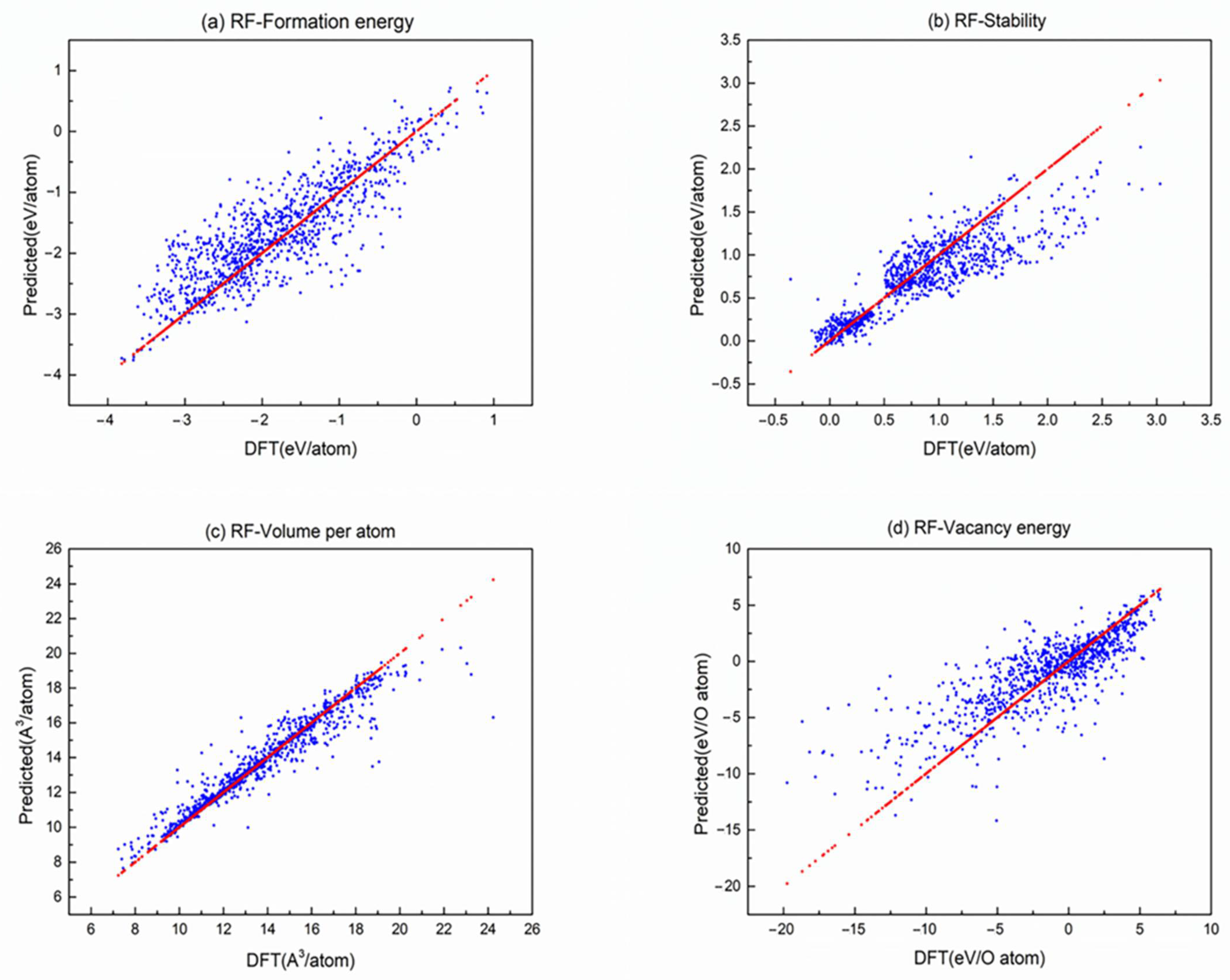
According to the above conclusions, the fitting diagram combining the predicted value of multiple algorithms and the calculated value of DFT are shown in Figure 4, Figure 5, Figure 6 and Figure 7. The horizontal axis is the calculated data of DFT, while the vertical axis is the predicted data. In Figure 4c, the points (DFT, Predicated) are closer to the reference points so that SVM-RBF has a better prediction effect on volume. In the same way, RF has a better prediction effect on volume, stability, and formation energy; RR has a better prediction effect on stability; and BPNN has a better prediction performance on these four characteristic parameters, which can effectively predict formation energy, stability, volume, and oxygen vacancy formation of perovskite materials.

The above results show that the prediction effect of different algorithms on different properties of material data is different. SVM-RBF can effectively predict the volume. RF can effectively predict the crystal volume, thermodynamic stability, and formation energy. RR can effectively predict the thermodynamic stability. BPNN can effectively predict the formation energy, thermodynamic stability, crystal volume, and oxygen vacancy formation energy. Therefore, the performance parameters in perovskite system which are difficult to be obtained by traditional experimental methods can be predicted by machine learning.

5. Conclusions

Four different machine learning algorithms, including support vector machine based on radial basis function (SVM-RBF), random forest (RF), ridge regression (RR), and BP neural network (BPNN), were used to predict the formation energy, stability, volume, and oxygen vacancy formation energy of perovskite materials. The algorithm model gets prediction results. SVM-RBF has a better prediction effect on the crystal volume; RF has a better prediction effect on the crystal volume, thermodynamic stability, and formation energy; RR has a better prediction effect on stability; and BPNN has a better prediction effect on all four characteristic parameters. It is further proved that different machine learning algorithms have different sensitivity to data, and different methods need to be selected to predict different performance parameters of perovskite materials. The machine learning method is applied to the performance prediction of perovskite materials, which improves the prediction efficiency and the subsequent performance prediction effect. The results have practical reference value for the study of machine learning methods in the performance prediction of perovskite materials and even in the research and development of new perovskite materials.

References

- Suntivich, J.; Gasteiger, H.A.; Yabuuchi, N.; Nakanishi, H.; Goodenough, J.B.; Shao-Horn, Y. Design principles for oxygen-reduction activity on perovskite oxide catalysts for fuel cells and metal–air batteries. Nat. Chem. 2011, 3, 546–550. [Google Scholar] [CrossRef]
- Suntivich, J.; May, K.; Gasteiger, H.A.; Goodenough, J.B.; Shao-Horn, Y. A Perovskite Oxide Optimized for Oxygen Evolution Catalysis from Molecular Orbital Principles. Science 2011, 334, 1383–1385. [Google Scholar] [CrossRef]
- Lee, M.M.; Teuscher, J.; Miyasaka, T.; Murakami, T.N.; Snaith, H.J. Efficient Hybrid Solar Cells Based on Meso-Superstructured Organometal Halide Perovskites. Science 2012, 338, 643–647. [Google Scholar] [CrossRef] [Green Version]
- Liu, M.; Johnston, M.; Snaith, H.J. Efficient planar heterojunction perovskite solar cells by vapour deposition. Nat. Cell Biol. 2013, 501, 395–398. [Google Scholar] [CrossRef]
- Bian, H.; Li, D.; Yan, J.; Liu, S.F. Perovskite—A wonder catalyst for solar hydrogen production. J. Energy Chem. 2021, 57, 325–340. [Google Scholar] [CrossRef]
- Cao, J.; Su, C.; Ji, Y.; Yang, G.; Shao, Z. Recent advances and perspectives of fluorite and perovskite-based dual-ion conducting solid oxide fuel cells. J. Energy Chem. 2021, 57, 406–427. [Google Scholar] [CrossRef]
- Hwang, J.; Rao, R.R.; Giordano, L.; Katayama, Y.; Yu, Y.; Shao-Horn, Y. Perovskites in catalysis and electrocatalysis. Science 2017, 358, 751–756. [Google Scholar] [CrossRef] [PubMed] [Green Version]
- Bednorz, J.G.; Müller, K.A. Possible high Tc superconductivity in the Ba-La-Cu-O system. Z. Phys. B Condens. Matter 1986, 64, 189–193. [Google Scholar] [CrossRef]
- Tao, S.; Irvine, J. A redox-stable efficient anode for solid-oxide fuel cells. Nat. Mater. 2003, 2, 320–323. [Google Scholar] [CrossRef]
- Ohtomo, A.; Hwang, H.Y. A high-mobility electron gas at the LaAlO3/SrTiO3 heterointerface. Nat. Cell Biol. 2004, 427, 423–426. [Google Scholar] [CrossRef] [PubMed]
- Kojima, A.; Teshima, K.; Shirai, Y.; Miyasaka, T. Organometal Halide Perovskites as Visible-Light Sensitizers for Photovoltaic Cells. J. Am. Chem. Soc. 2009, 131, 6050–6051. [Google Scholar] [CrossRef]
- Burschka, J.; Pellet, N.; Moon, S.-J.; Humphry-Baker, R.; Gao, P.; Nazeeruddin, M.K.; Grätzel, M. Sequential deposition as a route to high-performance perovskite-sensitized solar cells. Nat. Cell Biol. 2013, 499, 316–319. [Google Scholar] [CrossRef]
- Stranks, S.D.; Eperon, G.E.; Grancini, G.; Menelaou, C.; Alcocer, M.J.P.; Leijtens, T.; Herz, L.M.; Petrozza, A.; Snaith, H.J. Electron-Hole Diffusion Lengths Exceeding 1 Micrometer in an Organometal Trihalide Perovskite Absorber. Science 2013, 342, 341–344. [Google Scholar] [CrossRef] [PubMed] [Green Version]
- Besegatto, S.V.; da Silva, A.; Campos, C.E.M.; de Souza, S.M.A.G.U.; de Souza, A.A.U.; González, S.Y.G. Perovskite-based Ca-Ni-Fe oxides for azo pollutants fast abatement through dark catalysis. Appl. Catal. B Environ. 2021, 284, 119747. [Google Scholar] [CrossRef]
- Yashima, M.; Tsujiguchi, T.; Sakuda, Y.; Yasui, Y.; Zhou, Y.; Fujii, K.; Torii, S.; Kamiyama, T.; Skinner, S.J. High oxide-ion conductivity through the interstitial oxygen site in Ba7Nb4MoO20-based hexagonal perovskite related oxides. Nat. Commun. 2021, 12, 1–7. [Google Scholar] [CrossRef]
- Tao, Q.; Xu, P.; Li, M.; Lu, W. Machine learning for perovskite materials design and discovery. npj Comput. Mater. 2021, 7, 1–18. [Google Scholar] [CrossRef]
- Peña, M.A.; Fierro, J.L.G. Chemical Structures and Performance of Perovskite Oxides. Chem. Rev. 2001, 101, 1981–2018. [Google Scholar] [CrossRef] [PubMed]
- Fop, S.; McCombie, K.; Wildman, E.J.; Skakle, J.M.S.; Irvine, J.T.S.; Connor, P.A.; Savaniu, C.; Ritter, C.; McLaughlin, A.C. High oxide ion and proton conductivity in a disordered hexagonal perovskite. Nat. Mater. 2020, 19, 752–757. [Google Scholar] [CrossRef]
- Zhang, H.T.; Park, T.J.; Zaluzhnyy, I.A.; Wang, Q.; Wadekar, S.N.; Manna, S.; Andrawis, R.; Sprau, P.O.; Sun, Y.; Zhang, Z.; et al. Perovskite neural trees. Nat. Commun. 2020, 11, 2245. [Google Scholar] [CrossRef]
- Zhao, J.; Gao, J.; Li, W.; Qian, Y.; Shen, X.; Wang, X.; Shen, X.; Hu, Z.; Dong, C.; Huang, Q.; et al. A combinatory ferroelectric compound bridging simple ABO3 and A-site-ordered quadruple perovskite. Nat. Commun. 2021, 12, 747. [Google Scholar] [CrossRef]
- Butler, K.T.; Davies, D.W.; Cartwright, H.; Isayev, O.; Walsh, A. Machine learning for molecular and materials science. Nat. Cell Biol. 2018, 559, 547–555. [Google Scholar] [CrossRef]
- Pilania, G.; Wang, C.; Jiang, X.; Rajasekaran, S.; Ramprasad, R. Accelerating materials property predictions using machine learning. Sci. Rep. 2013, 3, 2810. [Google Scholar] [CrossRef]
- Raccuglia, P.; Elbert, K.C.; Adler, P.D.F.; Falk, C.; Wenny, M.B.; Mollo, A.; Zeller, M.; Friedler, S.A.; Schrier, J.; Norquist, A.J. Machine-learning-assisted materials discovery using failed experiments. Nat. Cell Biol. 2016, 533, 73–76. [Google Scholar] [CrossRef] [PubMed]
- Ramprasad, R.; Batra, R.; Pilania, G.; Mannodi-Kanakkithodi, A.; Kim, C. Machine learning in materials informatics: Recent applications and prospects. npj Comput. Mater. 2017, 3, 54. [Google Scholar] [CrossRef]
- Olivares-Amaya, R.; Amador-Bedolla, C.; Hachmann, J.; Atahan-Evrenk, S.; Sánchez-Carrera, R.S.; Vogt, L.; Aspuru-Guzik, A.; Vogt-Maranto, L. Accelerated computational discovery of high-performance materials for organic photovoltaics by means of cheminformatics. Energy Environ. Sci. 2011, 4, 4849–4861. [Google Scholar] [CrossRef] [Green Version]
- Tshitoyan, V.; Dagdelen, J.; Weston, L.; Dunn, A.; Rong, Z.; Kononova, O.; Persson, K.A.; Ceder, G.; Jain, A. Unsupervised word embeddings capture latent knowledge from materials science literature. Nat. Cell Biol. 2019, 571, 95–98. [Google Scholar] [CrossRef] [PubMed] [Green Version]
- Ren, F.; Ward, L.; Williams, T.; Laws, K.J.; Wolverton, C.; Hattrick-Simpers, J.; Mehta, A. Accelerated discovery of metallic glasses through iteration of machine learning and high-throughput experiments. Sci. Adv. 2018, 4, eaaq1566. [Google Scholar] [CrossRef] [Green Version]
- Juan, Y.; Dai, Y.; Yang, Y.; Zhang, J. Accelerating materials discovery using machine learning. J. Mater. Sci. Technol. 2021, 79, 178–190. [Google Scholar] [CrossRef]
- Tabor, D.P.; Roch, L.M.; Saikin, S.K.; Kreisbeck, C.; Sheberla, D.; Montoya, J.H.; Dwaraknath, S.; Aykol, M.; Ortiz, C.; Tribukait, H.; et al. Accelerating the discovery of materials for clean energy in the era of smart automation. Nat. Rev. Mater. 2018, 3, 5–20. [Google Scholar] [CrossRef] [Green Version]
- Ahn, J.J.; Lee, S.J.; Oh, K.J.; Kim, T.Y.; Lee, H.Y.; Kim, M.S. Machine learning algorithm selection for forecasting behavior of global institutional investors. In Proceedings of the 42nd Annual Hawaii International Conference on System Sciences, HICSS, Waikoloa, HI, USA, 5–8 January 2009. [Google Scholar]
- Portugal, I.; Alencar, P.; Cowan, D. The use of machine learning algorithms in recommender systems: A systematic review. Expert Syst. Appl. 2018, 97, 205–227. [Google Scholar] [CrossRef] [Green Version]
- Sharma, N.; Chawla, V.; Ram, N. Comparison of machine learning algorithms for the automatic programming of computer numerical control machine. Int. J. Data Netw. Sci. 2020, 4, 1–14. [Google Scholar] [CrossRef]
- Emery, A.A.; Wolverton, C. High-throughput DFT calculations of formation energy, stability and oxygen vacancy formation energy of ABO3 perovskites. Sci. Data 2017, 4, 170153. [Google Scholar] [CrossRef] [PubMed] [Green Version]
- Ye, W.; Chen, C.; Wang, Z.; Chu, I.-H.; Ong, S.P. Deep neural networks for accurate predictions of crystal stability. Nat. Commun. 2018, 9, 1–6. [Google Scholar] [CrossRef] [PubMed]
- Li, W.; Jacobs, R.; Morgan, D. Predicting the thermodynamic stability of perovskite oxides using machine learning models. Comput. Mater. Sci. 2018, 150, 454–463. [Google Scholar] [CrossRef] [Green Version]
- Ling, J.; Jones, R.; Templeton, J. Machine learning strategies for systems with invariance properties. J. Comput. Phys. 2016, 318, 22–35. [Google Scholar] [CrossRef] [Green Version]
- Schmidt, J.; Marques, M.R.G.; Botti, S.; Marques, M.A.L. Recent advances and applications of machine learning in solid-state materials science. npj Comput. Mater. 2019, 5, 83. [Google Scholar] [CrossRef]
- Maenhout, S.; De Baets, B.; Haesaert, G. Prediction of maize single-cross hybrid performance: Support vector machine regression versus best linear prediction. Theor. Appl. Genet. 2009, 120, 415–427. [Google Scholar] [CrossRef]
- Chen, Z.-B. Research on Application of Regression Least Squares Support Vector Machine on Performance Prediction of Hydraulic Excavator. J. Control Sci. Eng. 2014, 2014, 1–4. [Google Scholar] [CrossRef] [Green Version]
- Horvath, D.; Marcou, G.; Varnek, A.; Kayastha, S.; León, A.D.L.V.D.; Bajorath, J. Prediction of Activity Cliffs Using Condensed Graphs of Reaction Representations, Descriptor Recombination, Support Vector Machine Classification, and Support Vector Regression. J. Chem. Inf. Model. 2016, 56, 1631–1640. [Google Scholar] [CrossRef]
- Zang, Q.; Rotroff, D.; Judson, R.S. Binary Classification of a Large Collection of Environmental Chemicals from Estrogen Receptor Assays by Quantitative Structure–Activity Relationship and Machine Learning Methods. J. Chem. Inf. Model. 2013, 53, 3244–3261. [Google Scholar] [CrossRef]
- Pardakhti, M.; Moharreri, E.; Wanik, D.; Suib, S.L.; Srivastava, R. Machine Learning Using Combined Structural and Chemical Descriptors for Prediction of Methane Adsorption Performance of Metal Organic Frameworks (MOFs). ACS Comb. Sci. 2017, 19, 640–645. [Google Scholar] [CrossRef]
- Stamp, M. Introduction to Machine Learning with Applications in Information Security; CRC Press: Boca Raton, FL, USA, 2017. [Google Scholar]
- Wu, D.; Jennings, C.; Terpenny, J.; Gao, R.X.; Kumara, S. A Comparative Study on Machine Learning Algorithms for Smart Manufacturing: Tool Wear Prediction Using Random Forests. J. Manuf. Sci. Eng. 2017, 139, 071018. [Google Scholar] [CrossRef]
- Maronna, R.A. Robust Ridge Regression for High-Dimensional Data. Technometrics 2011, 53, 44–53. [Google Scholar] [CrossRef]
- Jain, A.; Hautier, G.; Ong, S.P.; Persson, K. New opportunities for materials informatics: Resources and data mining techniques for uncovering hidden relationships. J. Mater. Res. 2016, 31, 977–994. [Google Scholar] [CrossRef] [Green Version]
- Cherdantsev, D.V.; Stroev, A.V.; Mangalova, E.S.; Kononova, N.V.; Chubarova, O.V. The use of ridge regression for estimating the severity of acute pancreatitis. Bull. Sib. Med. 2019, 18, 107–115. [Google Scholar] [CrossRef]
- Feng, X.; Zhang, R.; Liu, M.; Liu, Q.; Li, F.; Yan, Z.; Zhou, F. An accurate regression of developmental stages for breast cancer based on transcriptomic biomarkers. Biomark. Med. 2019, 13, 5–15. [Google Scholar] [CrossRef] [PubMed]
- Zheng, W.D.; Zhang, H.R.; Hu, H.Q.; Liu, Y.; Li, S.Z.; Ding, G.T.; Zhang, J.C. Performance prediction of perovskite materials based on different machine learning algorithms. Zhongguo Youse Jinshu Xuebao/Chin. J. Non-Ferr. Met. 2019, 29, 803–809. [Google Scholar]
- Zou, Y.; Ding, Y.; Tang, J.; Guo, F.; Peng, L. FKRR-MVSF: A fuzzy kernel ridge regression model for identifying DNA-binding proteins by multi-view sequence features via chou’s five-step rule. Int. J. Mol. Sci. 2019, 20, 4175. [Google Scholar] [CrossRef] [Green Version]
- Suah, F.M.; Ahmad, M.; Taib, M.N. Applications of artificial neural network on signal processing of optical fibre pH sensor based on bromophenol blue doped with sol-gel film. Sens. Actuators B Chem. 2003, 90, 182–188. [Google Scholar] [CrossRef]
- Assarzadeh, S.; Ghoreishi, M. Neural-network-based modeling and optimization of the electro-discharge machining process. Int. J. Adv. Manuf. Technol. 2007, 39, 488–500. [Google Scholar] [CrossRef]
- Demetgul, M.; Tansel, I.; Taskin, S. Fault diagnosis of pneumatic systems with artificial neural network algorithms. Expert Syst. Appl. 2009, 36, 10512–10519. [Google Scholar] [CrossRef]
- Mandal, S.; Sivaprasad, P.; Venugopal, S.; Murthy, K. Artificial neural network modeling to evaluate and predict the deformation behavior of stainless steel type AISI 304L during hot torsion. Appl. Soft Comput. 2009, 9, 237–244. [Google Scholar] [CrossRef]
- Ahmadi, M.A.; Golshadi, M. Neural network based swarm concept for prediction asphaltene precipitation due to natural depletion. J. Pet. Sci. Eng. 2012, 98–99, 40–49. [Google Scholar] [CrossRef]
- Zhu, D.; Cheng, C.; Zhai, W.; Li, Y.; Li, S.; Chen, B. Multiscale Spatial Polygonal Object Granularity Factor Matching Method Based on BPNN. ISPRS Int. J. Geo-Inf. 2021, 10, 75. [Google Scholar] [CrossRef]
- Anjana, T.; Blas, U.P.; Christopher, S.R.; Ghanshyam, P. A Machine Learning Approach for the Prediction of Forma-bility and Thermodynamic Stability of Single and Double Perovskite Oxides. Chem. Mater. 2021, 33, 845–858. [Google Scholar]
- Zandi, S.; Saxena, P.; Razaghi, M.; Gorji, N.E. Simulation of CZTSSe Thin-Film Solar Cells in COMSOL: Three-Dimensional Optical, Electrical, and Thermal Models. IEEE J. Photovolt. 2020, 10, 1503–1507. [Google Scholar] [CrossRef]
Figure 1.
Machine learning flowchart in this experiment.
Figure 2.
Structure of BP neural networks.
Figure 3.
Prediction performance of machine learning model on test set, (a) prediction performance of formation energy, (b) prediction performance of stability, (c) prediction performance of volume, and (d) prediction performance of formation energy of oxygen vacancy.
Figure 4.
The fitting diagram based on the predicted value of SVM-RBF and the calculated value of DFT is (a) the fitting diagram of formation energy, (b) the fitting diagram of stability, (c) the fitting diagram of volume, and (d) the fitting diagram of oxygen vacancy formation energy. Red points work as reference points, which is ideal values obeyed y = x.
Figure 5.
Fitting diagram based on RF predicted value and DFT calculated value: (a) fitting diagram for formation energy, (b) fitting diagram for stability, (c) fitting diagram for volume, and (d) fitting diagram for formation energy of oxygen vacancy. Red points work as reference points, which is ideal values obeyed y = x.
Figure 6.
The fitting diagram based on the predicted value of RR and the calculated value of DFT is (a) the fitting diagram of formation energy, (b) the fitting diagram of stability, (c) the fitting diagram of volume, and (d) the fitting diagram of formation energy of oxygen vacancy. Red points work as reference points, which is ideal values obeyed y = x.
Figure 7.
The fitting diagram based on the predicted value of BPNN and the calculated value of DFT is (a) the fitting diagram of formation energy, (b) the fitting diagram of stability, (c) the fitting diagram of volume, and (d) the fitting diagram of formation energy of oxygen vacancy. Red points work as reference points, which is ideal values obeyed y = x.