Article

Application of General Full Factorial Statistical Experimental Design’s Approach for the Development of Sustainable Clay-Based Ceramics Incorporated with Malaysia’s Electric Arc Furnace Steel Slag Waste

by
Pao Ter Teo
1,*,
Siti Koriah Zakaria
1,
Nurulakmal Mohd Sharif
2,
Anasyida Abu Seman
2,
Mustaffa Ali Azhar Taib
3,
Julie Juliewatty Mohamed
1,
Mahani Yusoff
1,
Abdul Hafidz Yusoff
1,
Mardawani Mohamad
1,
Arlina Ali
1 and
Mohamad Najmi Masri
1
1
Faculty of Bioengineering and Technology, Universiti Malaysia Kelantan, Jeli Campus, Jeli 17600, Kelantan, Malaysia
2
School of Materials and Minerals Resources Engineering, Engineering Campus, Universiti Sains Malaysia, Seri Ampangan, Nibong Tebal 14300, Penang, Malaysia
3
Division of Advanced Ceramic Materials Technology, Advanced Technology Training Center (ADTEC) Taiping, Kamunting 34600, Perak, Malaysia
*
Author to whom correspondence should be addressed.
Crystals 2021, 11(4), 442; https://doi.org/10.3390/cryst11040442
Submission received: 14 March 2021 / Revised: 11 April 2021 / Accepted: 15 April 2021 / Published: 19 April 2021
(This article belongs to the Special Issue Recycling Silicate-Bearing Waste Materials)

Abstract

:
This study aims to optimize the composition (body formulation) and firing temperature of sustainable ceramic clay-based ceramics incorporated with electric arc furnace (EAF) steel slag waste using general full factorial design (GFFD). The optimization is necessary to minimize drawbacks of high iron oxide’s fluxing agent (originated from electric arc furnace, EAF steel slag waste), which led to severe surface defects and high closed porosity issue of the ceramics. Statistical analysis of GFFD including model adequacy checking, analysis of variance (ANOVA), interaction plots, regression model, contour plot and response optimizer were conducted in the study. The responses (final properties of ceramics) investigated were firing shrinkage, water absorption, apparent porosity, bulk density and modulus of rupture (MOR). Meanwhile, the factors employed in experimental parameters were weight percentage (wt.%) of EAF slag added and firing temperature. Upon statistical analysis, GFFD has deduced that wt.% amount of EAF slag added and firing temperatures are proven to significantly influence the final properties of the clay-based ceramic incorporated with EAF slag. The results of conducted statistical analysis were also highly significant and proven valid for the ceramics. Optimized properties (maximum MOR, minimum water absorption and apparent porosity) of the ceramic were attained at 50 wt.% of EAF slag added and firing temperature of 1180 °C.

1. Introduction

In recent years, the development of sustainable clay-based ceramics is becoming notable and attracting worldwide researchers to explore on it. A clay-based ceramic is regarded as ‘sustainable’ if it is made from waste materials (including by-products), environmentally friendly (non-hazardous and recyclable), energy-efficient and cost-effective [1,2,3,4,5,6,7]. Various worldwide researchers have proposed on the potential recycling of waste materials, such as blast furnace slag from the iron making process [8,9,10,11,12,13,14], waste glass [15,16,17,18,19,20,21,22,23,24,25,26,27], fly ash [28,29,30,31,32,33,34,35], sewage sludge [36,37,38,39,40,41,42,43,44,45,46,47,48,49] and electric arc furnace (EAF) steel slag from carbon steel making plant [4,50,51,52] as one of the raw materials for clay-based ceramic products such as brick, ceramic floor and wall tile as well as roofing tile. The idea of utilizing the waste materials for the ceramic body is progressively proposed due to they have proximate chemical composition to the natural resources (clay, flux and filler) used for conventional clay-based ceramics.
Badiee et al. (2008) [50], Sarkar et al. (2010) [51], Teo et al. (2014) [52] and Teo et al. (2019) [4] are among the pioneer researchers to initiate the idea of recycling EAF steel slag (by-product of carbon steel making) into sustainable clay-based ceramics. Although the research works were successful, they have mutually agreed that the high iron oxide content of EAF slag (25–42.4 wt.%) would cause vigorous fluxing action in the clay-based ceramic body. The iron oxide causes excessive formation of glassy phase, and the glassy phase would rapidly seal pores and trap gases, leading to surface defects such as bloating and blistering upon cooling of the ceramics [53]. Besides, the trapped gases would also remain as closed porosity in the ceramic body upon cooling. Therefore, combination of these drawbacks, surface defects and closed porosity would in turn deteriorate properties (water absorption and modulus of rupture) of the ceramics and these make the utilization of EAF slag is rather more challenging as compared to other waste materials. Owing to these, a thorough fine- tuning of formulation and firing temperature are required to minimize the drawbacks of high iron oxide in the slag. Although the EAF slag is suitable as a fluxing agent, the formulation of clay-based ceramics is still very crucial to avoid the drawbacks highlighted such as surface defects and closed porosity issues which could deteriorate properties (water absorption and MOR) of the tile. Considering this concern, proper formulation and firing temperature assisted by general full factorial design, which is one of a statistical experimental design approaches, could minimize the aforementioned drawbacks of clay-based ceramic incorporated with EAF slag.
Statistical experimental design is one of powerful data mining tools and could be considered as a black box of simulation with potential application in various research area [54]. It refers to the process of planning the experiment so that appropriate data will be collected and analyzed by statistical methods, resulting in a valid and objective conclusion. It is generally based on mathematical equations or models and outcomes of factors studied. Several types of commonly used experimental designs are Full Factorial Design, Fractional Factorial Design, General Full Factorial Design, Design of Mixture, Response Surface Methodology (RSM) and Taguchi Design. The selection of appropriate experimental design depends on objectives of the research and feasibility of experimental data, including factors or variables studied and outputs or responses targeted [55]. Each of the experimental design is accompanied with typical statistical methods such as model adequacy checking, analysis of variance (ANOVA), main effect and interaction plots, regression analysis, contour and surface plots and design optimizer [56,57]. To the best of the authors’ knowledge, the main objective of most previous DOE technique employed in the clay-based ceramics was merely to optimize composition of the green ceramics [58,59,60,61,62]. The composition optimized by them are shown in Table 1.
Since the design of a mixture experiment is merely limited to optimization of composition (body formulation) for the clay-based ceramics, general full factorial design has the advantages of an ability to screen more than one independent factors [63]. For example, the weight percentage of the raw material (composition/body formulation) and the firing temperature (processing parameter) are the independent factors employed in this research work. The general full factorial design has a certain level of flexibility in choosing the number of levels for each of assigned factor [64,65]. Thus, it is very useful when equality of levels may consist constraint towards obtaining more accurate predicted regression models [66]. Apart from that, through the general full factorial design, it is capable in determining which factors have significant effects in a response, as well as how the effect of one factor varies according to the level of other factors [67]. In this project, general full factorial design is very useful to study the effects of EAF slag and firing temperature on the properties of the clay-based green ceramics. Since the number of levels for the EAF slag and firing temperature are flexible, the flexibility of combined factors is also able to assist in the sintering mechanism study of the ceramics. Therefore, this study aims to fine- tune the formulation and firing temperature using a general full factorial design to further minimize the aforementioned drawbacks of clay-based green ceramics incorporated with EAF slag.

2. Materials and Methods

2.1. General Full Factorial Design (GFFD)

General Full Factorial Design (GFFD) is one of the statistical experimental design techniques. Its main purpose is to investigate the main effects and interaction of factors (parameters studied) run at different number of levels. In this project, the design was meant to investigate the effects of weight percentage of EAF slag (4 levels: 30 wt.%, 40 wt.%, 50 wt.% and 60 wt.%) and firing temperature (3 levels: 1100 °C, 1150 °C and 1180 °C) toon the final properties of the ceramic incorporated with the EAF slag waste, using statistical software package MINITAB 17, as shown in Table 2.
In the experimental design, there were several statistical analyses to be executed, such as ANOVA, normal probability plot, residual versus fits plot, interaction plot, contour plot and response optimizer. Table 2 shows the factors and their respective number of levels investigated in the general full factorial design. In terms of responses (final properties of the ceramic incorporated with EAF slag waste), the criteria evaluated were firing shrinkage (linear and volume), water absorption, apparent porosity, bulk density and modulus of rupture (MOR).

2.2. Run Experiment

Initially, EAF slag aggregate was collected from local steel manufacturers in Malaysia and was crushed into powder using a hardened steel ring mill for 15 min. The EAF slag powder was then sieved through 270 meshes, 53 µm (ASTM E11—16) test sieve to ensure only EAF slag with particle size equal to or less than 53 µm was used in the ceramic fabrication. Subsequently, the EAF slag powder was wet-mixed with ball clay for 1 h, with the presence of 0.05 wt.% sodium silicate deflocculant. The weight percentage (wt.%) of the EAF slag was varied according to the ‘run order’ in the design matrix, as shown in Table 3. After mixing, the slurry was further milled by ball milling with a hardened stainless-steel ball-to-slurry ratio of 10:1 for 5 h at 40 rpm. Then, the milled slurry was dried in an electric oven at 110 °C for 24 h. The dried mixture was then re-grinded using pestle and mortar for 1 h. After that, the powder mixture was moistened under a water spray. The amount of moisture introduced was approximately 5–6 wt.% per sample. Granulated mixture of each composition was compacted by hydraulic press with pressure of 40 MPa, producing a rectangular green body with dimensions 100 mm × 40 mm × 6 mm. The compacted body was dried in an electric oven at 110 °C for 24 h before firing at 1100 °C, 1150 °C and 1180 °C for 1 h, respectively. The firing’s sequence was according to the ‘run order’ in the design matrix (Table 3) as well. Finally, the naturally cooled ceramics were characterized accordingly in terms of firing shrinkage, water absorption, apparent porosity, bulk density, and modulus of rupture (MOR).
The firing shrinkage (linear and volume shrinkage) was determined by referring to ASTM C326-09 standard. The linear and volume shrinkages were calculated according to Equations (1) to (2), respectively.
Linear Shrinkage, Ls (%) = [(Lp − Lf)/Lp] × 100
Volume Shrinkage. Vs. (%) = {1 − [1 − (Ls/100)]3} × 100
where, Lp and Lf represent plastic length (before firing) and fired length (after firing) of the ceramic, respectively.
Meanwhile, the water absorption, apparent porosity and bulk density were determined by Archimedes principle as per the MS ISO 10545-3:2001 standard. First, mass of fired ceramic was determined and labelled as M1. The fired ceramic was then immersed in distilled water and placed in a vacuum chamber. It was evacuated to a pressure of approximately 100 kPa and maintained for 30 min, allowing water to impregnate into the ceramic. After impregnation, the suspended mass, M3 of the ceramic in water was determined. After weighing, the ceramic was wiped lightly with a cotton cloth to remove all excess water from its surface. Then, its saturated mass was determined and denoted as M2. The water absorption, apparent porosity and bulk density were calculated according to Equations (3)–(5), respectively.
Water absorption (%) = [(M2 − M1)/M1] × 100
Apparent porosity (%) = [(M2 − M1)/(M2 − M3)] × 100
Bulk Density (g/cm3) = M1/(M2 − M3)
where, M1, M2 and M3 represent mass of dried ceramic, saturated mass after immersion in water, and saturated mass during suspended in water, respectively.
MOR was determined by an Instron Testing Machine using a three-point bending system. The configuration of the testing and calculations were performed according to MS ISO 10545-4:2003 Standard. The MOR was calculated as in Equation (6).
MOR (MPa) = (3FL)/(2bd2)
where, F = load applied to rupture the specimen (N), L = span length between two supported rods (fixed at 100 mm), b = width of specimen (fixed at approximately 35 mm), d = thickness of specimen (fixed at approximately 4 mm).
Subsequently, all the quantitative results (linear shrinkage, volume shrinkage, water absorption, apparent porosity, bulk density and MOR) were tabulated in the design matrix (Table 3) before proceeding with the required statistical analyses.

3. Results and Discussion

3.1. Variables and Responses

General full factorial design (GFFD) with two independent variables or operating factors was used to statistically analyze effects of different operating factors and their interactions on predicted responses or properties (linear shrinkage, volume shrinkage, water absorption, apparent porosity, bulk density and MOR) of clay-based ceramics incorporated with the EAF slag. The independent variables were weight percentage (wt.%) of EAF slag and firing temperature, denoted as ‘A’ and ‘B’, respectively. As explained in Section 2.1, the weight percentage of EAF slag (factor A) had four levels, and each level was denoted in coded values of ‘1’, ‘2’, ‘’ and ‘4’. Meanwhile, for the firing temperature (factor B), it consisted of three levels, and the level was denoted as ‘1’, ‘2’ and ‘3’. The prediction of output responses or the quantitative properties of the ceramic tile were performed by fitting the experimental data to a regression model, as illustrated in Equation (7) below:
Y = β 0 + i = 1 k β i A i + j = 1 k β j B j + i = 1 k k = 1 k β ij A i B j
where, Y is a predicted response; Ai and Bi are independent coded variables; i and j are respective level for each variable, β0 is a constant; βi and βj are regression coefficient for linear effects; βij is regression coefficient for interaction effect.

3.2. Experimental Design Matrix

Table 3 shows experimental design matrix and experimental responses obtained from the total 24 experimental runs in random order with 2 replications. As mentioned earlier, coding was used to denote the level or range of each evaluated factor on a common scale of ‘1’, ‘2’, ‘3’ and ‘4’ for factor A and ‘1’, ‘2’, and ‘3’ for factor B. Subsequently, statistical analysis including model adequacy checking, analysis of variance (ANOVA), interaction plots, regression analysis, contour plot and responses optimizer were performed for each response, as shown in Section 3.3, Section 3.4, Section 3.5, Section 3.6, Section 3.7 and Section 3.8, respectively.

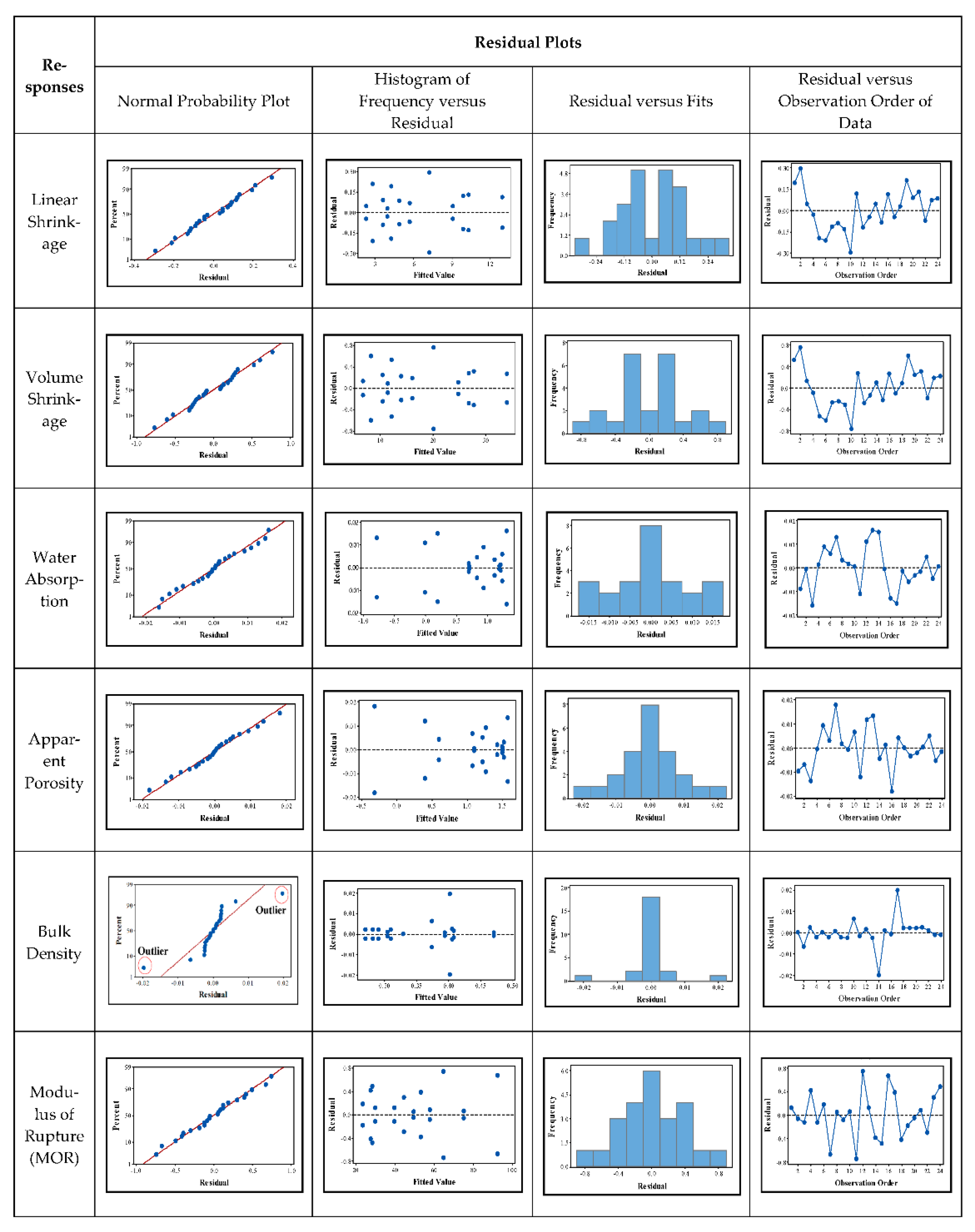
3.3. Model Adequacy Checking

Model adequacy checking was performed to verify several assumptions of residuals prior to further statistical analysis [55,68]. Generally, in statistical subjects, residuals can be defined as the difference of the actual and predicted response value [69]. In this case, the actual response values were obtained from the experimental run (as shown previously in Table 3) while the predicted response values were obtained from Equations (8)–(13) upon regression analysis, as shown in Table 5 of Section 3.6. The adequacy checking governs three assumptions of the residuals, (i) the normality assumption of the residuals, (ii) constant variance of the residuals, and (iii) independent assumption of the residuals. The adequacy of these assumptions would imply that the generated regression model (Equation (8) to Equation (13)) is mostly accurate for expressing the actual experimental data [70]. The three assumptions could be validated via several statistical residual plots, such as normal probability plot of residuals, histogram of frequency versus residuals, plot of residuals versus fitted or predicted values and plot of residuals in time sequence or observation order.
Figure 1 shows the residual plots for linear shrinkage, volume shrinkage, water absorption, apparent porosity, bulk density and modulus of rupture (MOR) of the clay-based ceramics incorporated with EAF slag. By analyzing all the normal probability plots, it was observed that most of the residual points are scattered along the straight line, except for bulk density. This indicated that the linear shrinkage, volume shrinkage, water absorption, apparent porosity and MOR data are normally distributed, and the first criteria of model adequacy checking were fulfilled [71]. The histogram plot also showed an almost symmetrical histogram bar, except for bulk density. Thus, this observation further supports the normal distribution of the linear shrinkage, volume shrinkage, water absorption, apparent porosity and MOR data [72].
Secondly, the residual versus fitted value plots illustrated that the data points for linear shrinkage, volume shrinkage, water absorption, apparent porosity and MOR are distributed randomly without significant structure, confirming the constant variance criteria of the residuals [70]. Conversely, the bulk density showed an obvious structure of the residuals’ distribution. In addition, residual versus observation order plots indicated that the residual points are completely random despite observation order, except for bulk density. This implies that the residuals were independent with each other and obeying the third assumption of the residuals mentioned earlier [70]. As mentioned earlier, the bulk density data displayed a non-normal trend compared to other responses. By observing again the normal probability plot of the bulk density (Figure 1), there were two outlier or unusual points present in the plot, leading to the non-normality of the data distribution. The outliers belong to a combination of 30 wt.% of EAF slag (Factor A, Level 1) and firing temperature of 1180 °C (Factor B, Level 3). In order to further investigate this issue, the Anderson–Darling normality test was performed on the bulk density data. The normality test was conducted before removing the outliers and after removing the outliers, as shown in Figure 2. Generally, null hypothesis (H0) of the normality test states that the data population is in a normal distribution [73]. In this case, our target was to accept the null hypothesis, and hence, the p-value has to be greater than 0.05. According to Figure 2, the p-value for the normality test prior to removal of outliers was less than 0.005, leading to rejection of the H0, and the data followed a non-normal distribution. However, after the outliers were removed, the p-value was increased to 0.326, contributing to the normality of the data distribution. Therefore, this confirmed the presence of the two mentioned outlier points.
In summary, since all assumptions of the residuals were mostly obeyed, the regression model generated in Section 3.6 (Equation (8) to Equation (13) of Table 5) could well express the experimental data for the linear shrinkage, volume shrinkage, water absorption, apparent porosity, bulk density and MOR.

3.4. Analysis of Variance (ANOVA)

In most of statistical experimental design, analysis of variance (ANOVA) method was conducted to evaluate significant effect of operating factors to properties or responses of a particular developed product or application [74,75,76]. In this case, through ANOVA, the significant effects of weight percentage of EAF slag (A) and firing temperature (B) on the responses, such as linear shrinkage, volume shrinkage, water absorption, apparent porosity, bulk density and MOR could be determined, by observing probability value, or also commonly known as ‘p-value’ upon the analysis. In general, the null hypothesis (H0) of ANOVA states that one or more than one operating factors do not cause a significant difference in means of any responses; H0: µ1 = µ2 = … = µa [55,77]. Most researchers have mutually agreed that the p-value has to be equal or smaller than 0.05 so that the operating factors are statistically significant in affecting the investigated response, leading to rejection of the null hypothesis for the ANOVA [71,72,74,75,76,78,79,80].
Table 4 shows the ANOVA for linear shrinkage, volume shrinkage, water absorption, apparent porosity, bulk density and MOR, respectively. The abbreviations of ‘DF’, ‘Adj. SS’, ‘Adj. MS’, ‘F-value’ and ‘p-value’ represent ‘degrees of freedom’, ‘adjusted sum of squares’, ‘adjusted mean squares’, ‘Fisher-value’ and ‘probability-value’, respectively. From the analysis, it was found that the p-value for ‘A’ and ‘B’ linear factors and also ‘A*B’ interaction factor is zero (0.000) for all responses or properties of the ceramic tile incorporated with the EAF slag. The smaller the p-value than did 0.05, the factor could be regarded to have a higher significant effect on the response [72]. Upon the analysis, it could be inferred that both wt.% of EAF slag (A) and firing temperature (B) operating factors significantly influence the linear shrinkage, volume shrinkage, water absorption, apparent porosity, bulk density and MOR of the clay-based ceramics incorporated with EAF slag.

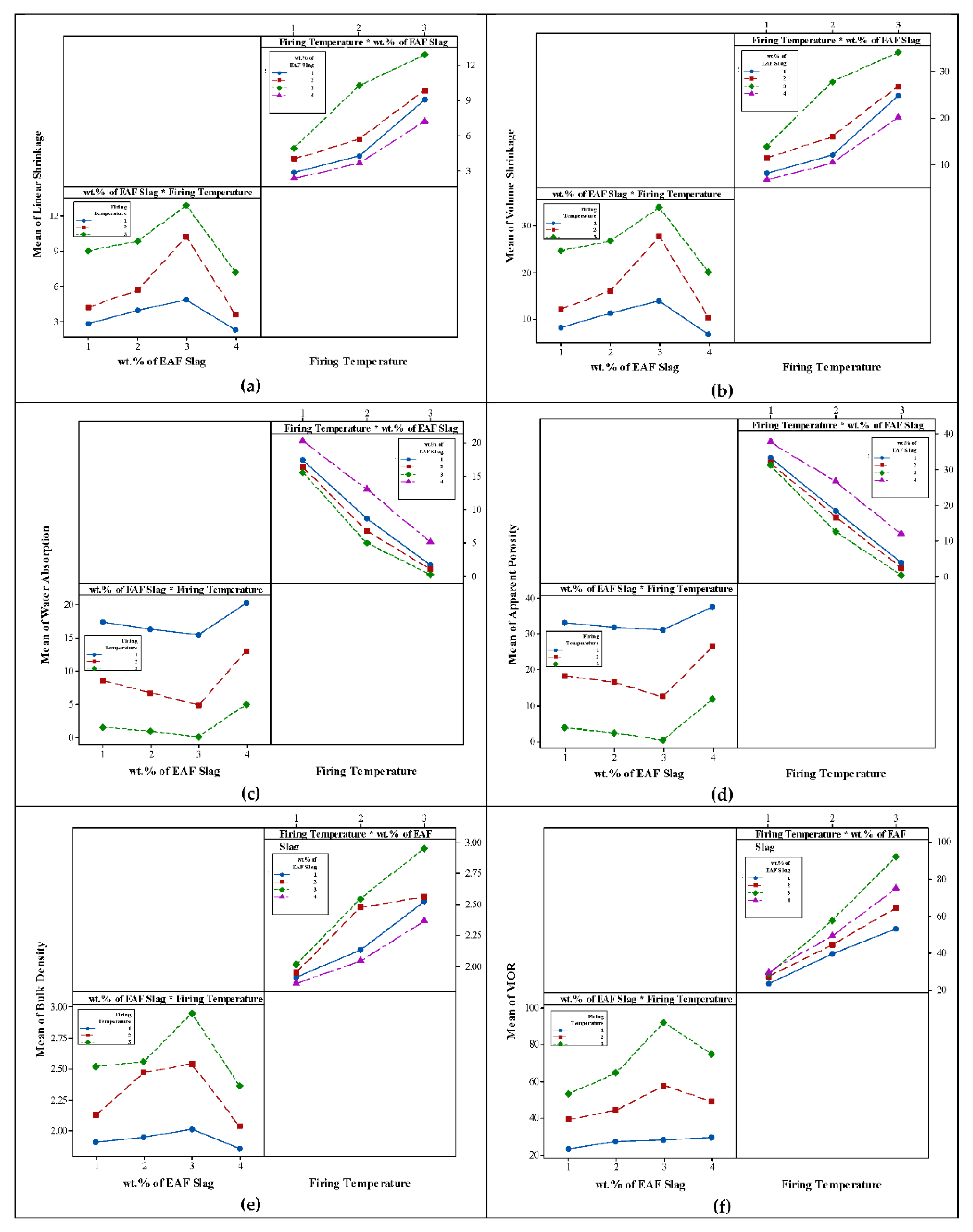
3.5. Interaction Plots

As mentioned previously in Section 3.1, in this general factorial design, the main factors evaluated were weight percentage (wt.%) of EAF slag and firing temperature. Interaction plot illustrates the combination effects of both main factors (with different levels) to the particular response (linear shrinkage, volume shrinkage, water absorption, apparent porosity, bulk density or MOR), as shown in Figure 3.

3.5.1. Firing Shrinkage (Linear and Volume Shrinkages)

Figure 3a,b shows the interaction plots for linear shrinkage and volume shrinkage, respectively. From the plots, it was observed that by increasing the weight percentage of EAF slag from 30 wt.% (coded as ‘1’) to 50 wt.% (coded as ‘3’), both the linear and volume shrinkages of the ceramics showed an increasing trend. However, further increasing the EAF slag to 60 wt.% (coded as ‘4’) reduced the linear and volume shrinkage of the ceramics. In terms of firing temperature, an increment of firing temperature from 1100 °C (coded as ‘1’) to 1180 °C (coded as ‘3’) led to an increasing trend of the linear and volume shrinkages.
On the other hand, the interaction plot also shows that the lines of the plot were not parallel with each other. Thus, this suggests that there is a strong interaction among the factors (weight percentage of EAF slag and firing temperature) studied in this experiment [81]. Upon interaction analysis, it was revealed that for all the weight percentage of EAF slag added, the linear and volume shrinkages of the ceramics increased with the firing temperature. The clay-based ceramics incorporated with 50 wt.% of EAF slag had the highest shrinkage among other compositions despite the different firing temperatures. In overall, the ceramics incorporated with 50 wt.% of EAF slag and fired at 1180 °C had the highest shrinkage among all.

3.5.2. Water Absorption, Apparent Porosity and Bulk Density

Figure 3c–e depict the interaction plots for water absorption, apparent porosity and bulk density, respectively. By observing the trend of the plots, it is revealed that the increment of EAF slag added from 30 wt.% (coded as ‘1’) to 50 wt.% (coded as ‘3’) contributes to reduction of water absorption and apparent porosity, accompanied by an increasing trend of bulk density in the clay-based ceramics incorporated with EAF slag. Furthermore, the water absorption and apparent porosity of the ceramics reduced with an increment of firing temperature used. This was also accompanied by an increase of bulk density of the ceramics. On the other hand, it could also be observed that interaction lines of the plots were not parallel with each other. As mentioned earlier, this deduced that both weight percentage of EAF slag and firing temperature had strong interaction, and they were simultaneously affecting the water absorption, apparent porosity and bulk density of the ceramics. Upon interaction analysis, it could be observed that regardless of composition, the water absorption and apparent porosity of the tile was lowest, and bulk density was highest at the highest firing temperature of 1180 °C. Meanwhile, the clay-based ceramics added with 50 wt.% of EAF slag had lower water absorption, apparent porosity and higher bulk density than other compositions at all the firing temperatures. In overall, the clay-based ceramics added with 50 wt.% of EAF slag and fired at 1180 °C had the lowest water absorption, apparent porosity and highest bulk density.

3.5.3. Modulus of Rupture (MOR)

Figure 3f shows the interaction plots for MOR of the clay-based ceramics incorporated with EAF slag. From the plots, it could be seen that as the EAF slag added was increased from 30 wt.% (coded as ‘1’) to 50 wt.% (coded as ‘3’), the MOR increased. However, further increment of the EAF slag added to 60 wt.% (coded as ‘4’) deteriorate the MOR. In terms of firing temperature, MOR increased with the firing temperature. Besides, it could also be observed that both factors (weight percentage of EAF slag and firing temperature) had an interaction effect on the MOR as the lines were not parallel with each other. Regardless of the weight percentage of EAF slag, the MOR increased with the firing temperature. The clay-based ceramics added with 50 wt.% of EAF slag had the highest MOR, while those added with 30 wt.% of EAF slag had the lowest MOR for all firing temperatures. In overall, the clay-based ceramics added with 50 wt.% of EAF slag and fired at 1180 °C had the highest MOR, while the ceramics added with 30 wt.% of EAF slag and fired at 1100 °C had the lowest MOR.

3.6. Regression Analysis

Apart from interaction plots, there is another alternative to express the effect of operating factors on particular responses in a quantitative approach. This could be achieved via regression model analysis [55,82], as shown in Table 5. The regression analysis includes correlation of coefficient (R2), coefficient of each factor, values of constant, p-value and subsequently, regression equation. The correlation of coefficient (R2) and regression equation are tabulated in Table 5. Meanwhile, the complete details of coefficient of each factor, values of constant and p-value are shown in Appendix A. The p-value would indicate the significance of this constant and regression coefficient in the developed regression model.

3.6.1. Firing Shrinkages (Linear and Volume Shrinkages)

The regression analysis for linear and volume shrinkages is presented in Table 5 and Appendix A. For the linear shrinkage, the value of constant was found to be 6.4017 with its p-value of zero (0.000), indicating its significant in the regression model (Equation (8)). Meanwhile, the p-value for coefficients of factor A (weight percentage of EAF slag) was less than 0.05, except for level 2 (40 wt.% EAF slag) with its p-value of 0.175. For factor B (firing temperature), the p-value was less than 0.05 for all levels. For interaction terms (A*B), most combinations had p-value less than 0.05, except for A2*B3 (combination of 40 wt.% EAF slag with firing temperature of 1180 °C) and A3*B3 (combination of 50 wt.% EAF slag with firing temperature of 1180 °C).
Meanwhile, for volume shrinkage, the value of constant was 17.697. It was significant in the regression model (Equation (9)) as its p-value was 0.000. For factor A (weight percentage of EAF slag), the p-values were less than 0.05, except for level 2 (40 wt.%) with its slightly higher p-value of 0.057. For factor B, all the p-value were 0.000. In addition, for the interaction terms (A*B), most interactions had p-value less than 0.05, except for A2*B3 (combination of 40 wt.% EAF slag with firing temperature of 1180 °C) and A3*B3 (combination of 50 wt.% EAF slag with firing temperature of 1180 °C).
Although certain coefficient of factors and their interaction terms (for both linear and volume shrinkage) had p-value greater than 0.05, this is not a single criterion to reject the generated regression model. Alternatively, the significant level of the regression equation is also dependent on R2 (correlation of coefficient) value of the developed model. In the regression analysis, R2 would provide correlation between experimental response (obtained from experimental run) and predicted response (obtained from regression model). Therefore, the closer the R2 value to 100%, the higher the precision level of the developed regression model [83]. In other words, the regression model could effectively represent the experimental data. From Table 5, the R2 value for the linear and volume shrinkages regression equation was 99.81%, and it was closed to 100%. This indicates that up to 99.81% of variation in the linear and volume shrinkages experimental data could be well explained by the Equations (8) and (9) regression model [66].
Apart from R2 value, adjusted R2 or commonly denoted as R2 (adj.) is another criterion to evaluate the degree of accuracy of the regression model [79]. R2 (adj.) is a correction of R2 by considering sample size and number of terms in the regression equation [83]. From the analysis, the linear and volume shrinkages shrinkage regression model had R2 (adj.) value of 99.65% and 99.63% respectively. Thus, it could be deduced that the accuracy of both models is 99.65% and 99.63% respectively. Both models could well represent the actual experimental data of linear and volume shrinkage. Besides that, predicted R2 or commonly known as R2 (pred.) of the linear and volume shrinkage was 99.26% and 99.22%. This indicated that 99.26% of the linear shrinkage data and 99.22% of the volume shrinkage data could be predicted by the respective regression models (Equations (8) and (9)). Palkar and Shilapuram (2015) [54] have proposed that the difference between R2 (adj.) and R2 (pred.) has to be less than 20, so that the developed regression model is highly reliable. From the analysis, it was found that the difference of R2 (adj.) and R2 (pred.) for the linear shrinkage is 0.39, while it was 0.41 for volume shrinkage. In overall, from the p-value, R2, R2 (adj.) and R2 (pred.) criterions, it could be deduced that the developed regression models (Equations (8) and (9)) for the linear and volume shrinkages were highly significant.

3.6.2. Water Absorption, Apparent Porosity and Bulk Density

Table 5 and Appendix A also depict the regression analysis for water absorption, apparent porosity and bulk density. Values of constant for the water absorption, apparent porosity and bulk density were 9.2183, 18.9220 and 2.2775 respectively. p-Values for the constants were 0.000, indicating that the constants were significant in the regression models (Equations (10)–(12)). For water absorption, the p-value for the coefficient of factor A (weight percentage of EAF slag) was less than 0.05, except for level 1 (30 wt.%), which had a p-value of 0.912. p-Values for coefficient of factor B (firing temperature) were 0.000. In terms of coefficient for interaction factors (A*B), there were several interactions that experienced slightly higher p-value than 0.05. The interactions were A1*B1, A1*B2, A1*B3, A2*B1 and A2*B3 with p-values of 0.823, 0.082, 0.055, 0.335 and 0.189 respectively.
For apparent porosity, the coefficient of factor A (weight percentage of EAF slag) had p-values less than 0.05, except for level 1 (30 wt.% of EAF slag), while the p-values for coefficient of factor B (firing temperature) were entirely less than 0.05. For the interaction term (A*B), there were certain coefficients which had a p-value higher than 0.05. The terms were A1*B1, A1*B2, A1*B3, A2*B1, A2*B2, A2*B3 and A3*B3 with their p-values of 0.614, 0.421, 0.202, 0.303, 0.913, 0.258 and 0.777 respectively. On the other hand, for bulk density, the p-values for the coefficient of factor A (weight percentage of EAF slag) were lower than 0.05. Meanwhile, coefficient of factor B (firing temperature) had the p-value smaller than 0.05 too, except for level 2 (1150 °C). In terms of interaction factor, a few of the coefficients for the interactions experienced p-values greater than 0.05. The interaction terms were A1*B3, A2*B1, A3*B2 and A4*B3 with their respective p-values of 0.618, 0.195, 0.443 and 0.086.
Similarly, although certain coefficients of water absorption, apparent porosity and bulk density had p-value greater than 0.05, this is not a single justification to reject the regression models developed. Other statistical parameters such as R2, R2 (adj.) and R2 (pred.) would also have to be considered. From the regression analysis, it was observed that the regression model of water absorption, apparent porosity and bulk density had a high R2 value of 99.88%, 99.9% and 98.82% respectively. This indicated that up to 99.88% of the water absorption experimental data, 99.91% of the apparent porosity experimental data, and 98.82% of the bulk density experimental data could be represented by the respective regression models (Equations (10)–(12)). In terms of accuracy of the developed regression models, water absorption’s regression had R2 (adj.) value of 99.76%, while the apparent porosity and bulk density with R2 (adj.) of 99.83% and 97.75%, respectively. With these large values of R2 (adj.), it can be said that the regression models had high accuracy, and they could well represent the actual experimental data. In addition, the regression models for water absorption, apparent porosity and bulk density also possessed a large value of R2 (pred.) with 99.50%, 99.64% and 95.30% respectively. This deduced that high probability of the water absorption, apparent porosity and bulk density data to be predicted by the regression models. In addition, the difference between R2 (adj.) and R2 (pred.) for water absorption, apparent porosity and bulk density were 0.26, 0.19 and 0.45, respectively, which were far lower than 20. Thus, the regression models are highly reliable in expressing the experimental data. In overall, considering the p-value, R2, R2 (adj.) and R2 (pred.) criterions, it could be said that the generated regression models (Equations (10)–(12)) were highly significant.

3.6.3. Modulus of Rupture (MOR)

Regression analysis of MOR for ceramic tile incorporated with EAF slag is also presented in Table 5 and Appendix A. Upon the regression analysis, it was found that p-value for the constant in the regression equation (Equation (13)) was 48.870 with p-value of 0.000. For interaction terms (A*B), only two coefficients of the interactions had p-value greater than 0.05. The terms were A2*B2 and A4*B1 with their p-values of 0.708 and 0.543 respectively. As mentioned previously, apart from evaluating the p-value for coefficient of the regression equation, R2, R2 (adj.) and R2 (pred.) were also important statistical criterions to be considered in order to justify the particular regression model. For the MOR, its regression model possessed R2, R2 (adj.) and R2 (pred.) of 99.96%, 99.93% and 99.86% respectively. This conveyed that the model could well represent the actual experimental data with high accuracy and also able to firmly predict the MOR’s experimental data. The small difference (0.09) between the R2 (adj.) and R2 (pred.) further support the reliability of the model in expressing the MOR experimental data. In overall, considering all the statistical criterions, it could be inferred that the MOR’s regression model (Equation (13)) was highly significant.

3.6.4. Correlation between Firing Shrinkage, Water Absorption, Apparent Porosity, Bulk Density and MOR

According to the correlations in Figure 3, it could be observed that changes of weight percentage of EAF slag and firing temperature did significantly influence the linear and volume shrinkage of the ceramics. Increment of firing temperature from 1100 to 1180 °C increased both linear and volume shrinkage of the ceramics. Meanwhile, the shrinkage increased with added EAF slag from 30 to 50 wt.%. It was also observed that the shrinkage reduced with further addition of EAF slag (60 wt.%). The variations in linear and volume shrinkage of the ceramics were closely related with bulk density, apparent porosity, water absorption and MOR of the ceramics.
Based on the correlation analysis in Figure 3, as linear and volume shrinkage increased, the bulk density increased, accompanied by reduction of apparent porosity and water absorption. During firing process, iron oxide (FeO) content of EAF slag reacted with silicates and alumina-silicates present in ceramic powder mixture and the formed compounds began to melt into glassy phase, or also known as a viscous liquid [4,52]. As firing temperature was increased up to 1180 °C, and EAF slag added was increased up to 50 wt.%, a greater amount of glassy phase was formed, and penetrating the pores. Subsequently, the glassy phase closed-up the pores and isolating neighboring pores. The liquid surface tension and capillary effects of the glassy phase would then bring pores closer together. Therefore, this would reduce the apparent porosity, and densified (increment of bulk density) the ceramic body [84,85,86]. Due to these phenomena, the ceramic would then possess higher shrinkage and lower water absorption properties.
Besides, the MOR was also correlated with apparent porosity to explain the synergistic effect of the porosity to the MOR of the ceramics, as shown in the previous Figure 3. It could be observed that the reduction of apparent porosity reduced the MOR of the ceramics. This could be explained in terms of fracture mechanic mechanism. According to principle of materials fracture mechanic, pores present would act as stress concentration points, and they are likely to initiate crack in ceramic bodies. Therefore, ceramics with higher apparent porosity would possess weaker points and subsequently reducing the MOR’s mechanical strength [87,88,89].

3.7. Contour Plot and Its Application

Contour plot is a graphical representation of the regression model [72], showing prediction of responses (linear shrinkage, volume shrinkage, water absorption, apparent porosity, bulk density and MOR) according to desired factors (weight percentage of EAF slag and firing temperature). The contour plots for linear shrinkage, volume shrinkage, water absorption, apparent porosity, bulk density and MOR are shown in Figure 4. It could be observed that all the contour plots consisted of contour or curve lines. This further support the presence of interaction between the weight percentage of EAF slag (factor A) and firing temperature (factor B).
Since different batches of EAF slag had slight variation in their chemical composition, especially total iron (Fe), calcium oxide (CaO), silicon dioxide (SiO2) and aluminum oxide (Al2O3), and these might cause inconsistency of the final properties of the clay-based ceramics [84], contour plot would be useful in evaluating the significant effects of the chemical composition’s variation to the final properties of clay-based ceramics incorporated with EAF slag. Clay-based ceramics added with 50 wt.% of EAF slag and fired at 1180 °C, were re-fabricated using a new batch of EAF slag. These parameters were chosen because the ceramics had the best properties (the lowest water absorption, apparent porosity and highest MOR) among others.
From the contour plots, it was predicted that clay-based ceramics added with 50 wt.% of EAF slag (coded as ‘3’) and fired at 1180 °C (coded as ‘3’) has the highest linear shrinkage (greater than 12%) and volume shrinkage (greater than 30%), the lowest water absorption (less than 5%) and apparent porosity (less than 5%), the highest bulk density (more than 2.8 g/cm3) and MOR (greater than 90 MPa), as tabulated in Table 6. Subsequently, the properties of the re-fabricated are also tabulated in Table 6 and compared with the predicted data from the contour plot.
From the Table 6, it was observed that the properties (linear shrinkage, volume shrinkage, water absorption, apparent porosity, bulk density and MOR) of the re-fabricated ceramics follow the trend of the predicted data (contour plot). Thus, it could be deduced that the different batches of EAF slag is unlikely to significantly alter and deteriorate the final properties of the clay-based ceramics incorporated with EAF slag.

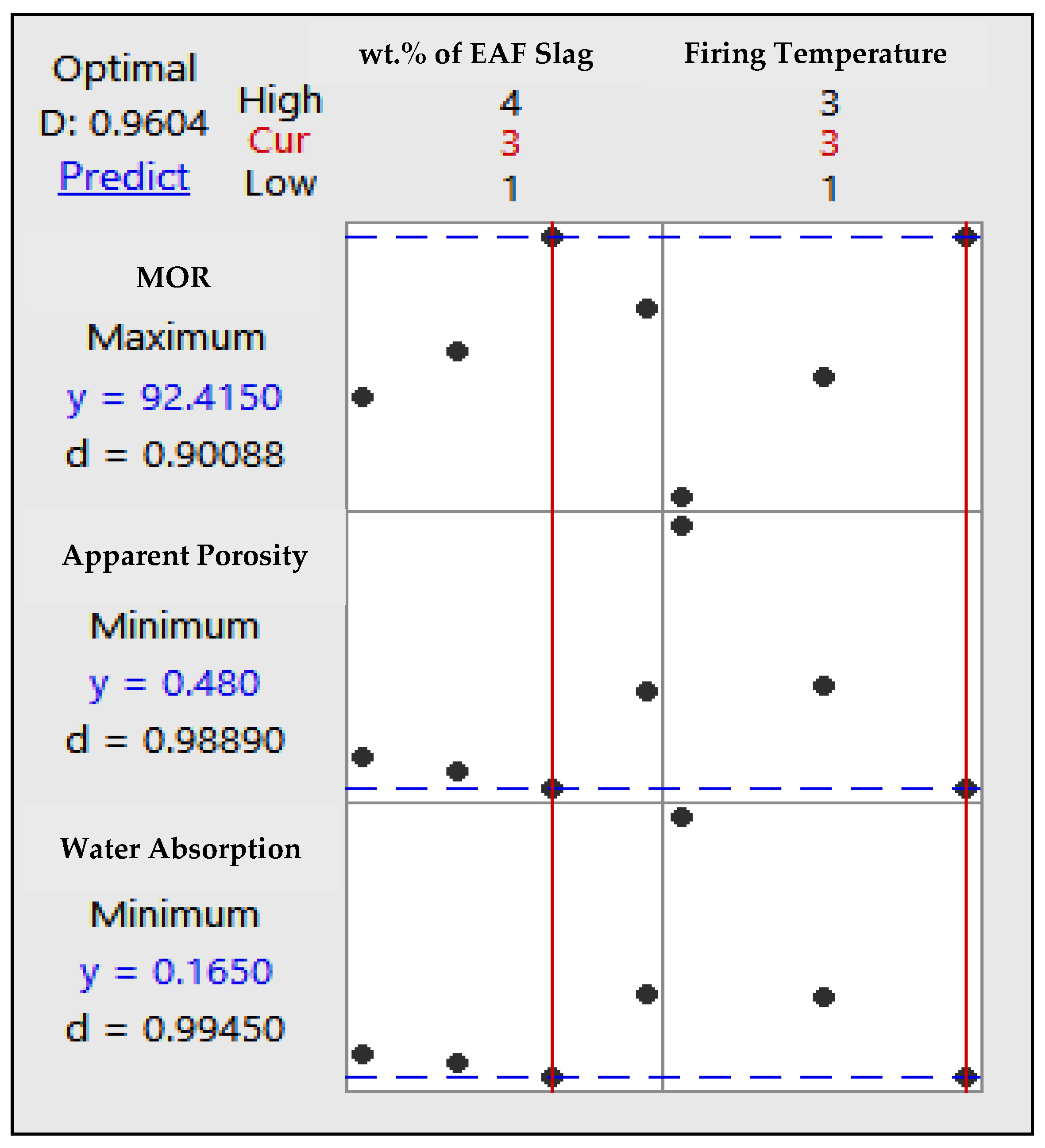
3.8. Response Optimizer

From the regression model developed, the optimal condition of controlled variables or factors could be determined in order to produce desired properties of ceramic tile incorporated with EAF slag, using responses optimizer in MINITAB 17. In this case, three responses (MOR, water absorption and apparent porosity) were targeted. The targets were to achieve maximum MOR, minimum water absorption and apparent porosity. Figure 5 shows the optimization plot for the desired responses.
Upon the analysis, it was predicted that the maximum MOR, minimum water absorption and apparent porosity were 92.415 MPa, 0.480% and 0.165% respectively. These desired responses were achieved at 50 wt.% of EAF slag (coded as ‘3’) and firing temperature of 1180 °C (coded as ‘3’) with composite desirability (D) greater than 0.90 and closer to 1.00. Composite desirability (D) is another statistical parameter to validate accuracy of the optimization plot [81]. According to Chang et al. (2015) [90,91,92,93], the closer the composite desirability (D) to 1.00, the optimization of factors and responses obtained from the statistical analysis is highly reliable and accurate. Hence, the optimal conditions proposed in the optimization plot (Figure 4) were mostly reliable, and they fully obeyed the regression models developed.

4. Conclusions

At the end of this research work, the general full factorial design (GFFD) statistical experimental design’s approach successfully optimized EAF slag added and firing temperature for the development of sustainable clay-based ceramic incorporated with EAF slag. Several conclusions could be addressed based on the GFFD’s statistical analysis:
  • Weight percentage of EAF slag added and firing temperatures were statistically proven to significantly influence final properties (firing shrinkage, water absorption, apparent porosity, bulk density and MOR) of the clay-based ceramic incorporated with EAF slag.
  • The results of statistical analysis including model adequacy checking, analysis of variance (ANOVA), interaction plots, regression model, and contour plots were highly significant and proven for the clay-based ceramic incorporated with EAF slag.
  • The optimized properties (maximum MOR, minimum water absorption and apparent porosity) of the clay-based ceramic incorporated with EAF slag were attained at 50 wt.% of EAF slag added and firing temperature of 1180 °C.

Author Contributions

Conceptualization, P.T.T.; Formal analysis, M.M., A.A. and M.N.M.; Funding acquisition, A.H.Y.; Investigation, S.K.Z.; Methodology, N.M.S. and A.A.S.; Project administration and Validation, P.T.T.; Resources, M.A.A.T., J.J.M. and M.Y.; Supervision, P.T.T.; Writing—original draft, S.K.Z.; Writing—review &and editing, A.H.Y. All authors have read and agreed to the published version of the manuscript.

Funding

This research was funded by Fundamental Research Grant Scheme (FRGS), Ministry of Higher Education Malaysia (Grant No: R/FRGS/A1300/01687A/001/2018/00549) and the article processing fees (APC) was funded by Publication and Rating Division, Research Management and Innovation Centre, Office of Deputy Vice Chancellor (Research and Innovation), Universiti Malaysia Kelantan.

Institutional Review Board Statement

Not applicable.

Informed Consent Statement

Not applicable.

Data Availability Statement

The data presented in this study are available on request from the corresponding author. The data are not publicly available due to restricted by policies of intellectual property (IP), i.e., Patent filing.

Acknowledgments

The authors would like to convey their heartfelt gratitude to Faculty of Bioengineering and Technology, Universiti Malaysia Kelantan for providing research facilities to complete this research work.

Conflicts of Interest

The authors declare no conflict of interest.

Appendix A

(i)
Estimated regression coefficient, correlation of coefficient (R2) and regression equation for linear shrinkage
TermCoefficientSE Coefficientp-Value
Constant6.40170.04070.000
A
 1−1.03500.07050.000
 20.10170.07050.175
 32.96500.07050.000
 4−2.03170.07050.000
B
 1−2.91920.05760.000
 2−0.45290.05760.000
 33.37210.05760.000
A*B
 1*10.35250.09980.004
 1*2−0.67880.09980.000
 1*30.32630.09980.007
 2*10.36580.09980.003
 2*2−0.37040.09980.003
 2*30.00460.09980.964
 3*1−1.56250.09980.000
 3*21.36620.09980.000
 3*30.19630.09980.073
 4*10.84420.09980.000
 4*2−0.21710.09980.008
4*3−0.52710.09980.000
R2 = 99.81%R2 (adj.) = 99.65%R2 (pred.) = 99.26%
Regression Equation: 6.4017 − 1.0350 [A_1] + 0.1017 [A_2] + 2.9650 [A_3] − 2.0317 [A_4] − 2.9192 [B_1] − 0.4529 [B_2] + 3.3721 [B_3] + 0.3525 [A_1*B_1] − 0.6788 [A_1*B_2] + 0.3263 [A_1*B_3] + 0.3658 [A_2*B_1] − 0.3704 [A_2*B_2] + 0.0046 [A_2*B_3] − 1.5625 [A_3*B_1] + 1.3662 [A_3*B_2] + 0.1963 [A_3*B_3] + 0.8442 [A_4*B_1] − 0.3171 [A_4*B_2] − 0.5271 [A_4*B_3]
(Equation (8))
(ii)
Estimated regression coefficient, correlation of coefficient (R2) and regression equation for volume shrinkage
TermCoefficientSE Coefficientp-Value
Constant17.69700.10800.000
A
 1−2.65400.18600.000
 20.39300.18600.057
 37.53800.18600.000
 4−5.27700.18600.000
B
 1−7.63600.15200.000
 2−1.09000.15200.000
 38.72500.15200.000
A*B
 1*10.75800.26300.014
 1*2−1.78400.26300.000
 1*31.02600.26300.002
 2*10.94100.26300.004
 2*2−0.92000.26300.004
 2*3−0.02000.26300.939
 3*1−3.65400.26300.000
 3*23.62000.26300.000
 3*30.03500.26300.898
 4*11.95600.26300.000
 4*2−0.91500.26300.005
4*3−1.04000.26300.002
R2 = 99.81%R2 (adj.) = 99.63%R2 (pred.) = 99.22%
Regression Equation: 17.6970 − 2.6540 [A_1] + 0.3930 [A_2] + 7.5380 [A_3] − 5.2770 [A_4] − 7.6360 [B_1] − 1.090 [B_2] + 8.7250 [B_3] + 0.7580 [A_1*B_1] − 1.7840 [A_1*B_2] + 1.0260 [A_1*B_3] + 0.9410 [A_2*B_1] − 0.9200 [A_2*B_2] − 0.0200 [A_2*B_3] − 3.6540 [A_3*B_1] + 3.6200 [A_3*B_2] + 0.035 [A_3*B_3] + 1.9560 [A_4*B_1] − 0.9150 [A_4*B_2] − 1.040 [A_4*B_3]
(Equation (9))
(iii)
Estimated regression coefficient, correlation of coefficient (R2) and regression equation for water absorption
TermCoefficientSE Coefficientp-Value
Constant9.21830.06840.000
A
 1−0.01300.11900.912
 2−1.19300.11900.000
 3−2.34000.11900.000
 43.54700.11900.000
B
 18.14670.09680.000
 2−0.87330.09680.000
 3−7.27330.09680.000
A*B
 1*10.03800.16800.823
 1*20.31800.16800.082
 1*3−0.35700.16800.055
 2*10.16800.16800.335
 2*2−0.40200.16800.034
 2*30.23300.16800.189
 3*10.50500.16800.011
 3*2−1.0650.16800.000
 3*30.56000.16800.006
 4*1−0.71200.16800.001
 4*21.14800.16800.000
4*3−0.43700.16800.023
R2 = 99.88%R2 (adj.) = 99.76%R2 (pred.) = 99.50%
Regression Equation: 9.2183 − 0.0130 [A_1] − 1.1930 [A_2] − 2.3400 [A_3] + 3.5470 [A_4] + 8.1467 [B_1] − 0.8733 [B_2] − 7.2733 [B_3] + 0.0380 [A_1*B_1] + 0.3180 [A_1*B_2] − 0.3570 [A_1*B_3] + 0.1680 [A_2*B_1] − 0.4020 [A_2*B_2] + 0.2330 [A_2*B_3] + 0.5050 [A_3*B_1] − 1.0650 [A_3*B_2] + 0.5600 [A_3*B_3] − 0.7120 [A_4*B_1] + 1.1480 [A_4*B_2] − 0.4370 [A_4*B_3]
(Equation (10))
(iv)
Estimated regression coefficient, correlation of coefficient (R2) and regression equation for apparent porosity
TermCoefficientSE Coefficientp-Value
Constant18.92200.10900.000
A
 1−0.39900.18800.055
 2−1.89200.18800.000
 3−4.17000.18800.000
 46.46100.18800.000
B
 114.54900.15300.000
 2−0.35500.15300.039
 3−14.19500.15300.000
A*B
 1*10.13800.26600.614
 1*20.22100.26600.421
 1*3−0.35900.26600.202
 2*10.28600.26600.303
 2*20.03000.26600.913
 2*3−0.31500.26600.258
 3*11.89900.26600.000
 3*2−1.82200.26600.000
 3*3−0.07700.26600.777
 4*1−2.32200.26600.000
 4*21.57100.26600.000
4*30.75100.26600.015
R2 = 99.91%R2 (adj.) = 99.83%R2 (pred.) = 99.64%
Regression Equation: 18.9220 − 0.3990 [A_1] − 1.8920 [A_2] − 4.1700 [A_3] + 6.4610 [A_4] + 14.5490 [B_1] − 0.3550 [B_2] − 14.1950 [B_3] + 0.1380 [A_1*B_1] + 0.2210 [A_1*B_2] − 0.3590 [A_1*B_3] + 0.2860 [A_2*B_1] + 0.0300 [A_2*B_2] − 0.3150 [A_2*B_3] + 1.8990 [A_3*B_1] − 1.8220 [A_3*B_2] − 0.0770 [A_3*B_3] − 2.3220 [A_4*B_1] + 1.5710 [A_4*B_2] + 0.7510 [A_4*B_3]
(Equation (11))
(v)
Estimated regression coefficient, correlation of coefficient (R2) and regression equation for bulk density
TermCoefficientSE Coefficientp-Value
Constant2.27750.01030.000
A
 1−0.08920.01780.000
 20.05080.01780.015
 30.22750.01780.000
 4−0.18920.01780.000
B
 1−0.34380.01460.000
 20.02000.01460.194
 30.32380.01460.000
A*B
 1*10.06540.02520.023
 1*2−0.07830.02520.009
 1*30.01290.02520.618
 2*1−0.03460.02520.195
 2*20.12670.02520.000
 2*3−0.09210.02520.003
 3*1−0.14630.02520.000
 3*20.02000.02520.443
 3*30.12630.02520.000
 4*10.11540.02520.001
 4*2−0.06830.02520.019
4*3−0.04710.02520.086
R2 = 98.82%R2 (adj.) = 97.75%R2 (pred.) = 95.30%
Regression Equation: 2.2775 − 0.0892 [A_1] + 0.0508 [A_2] + 0.2275 [A_3] − 0.1892 [A_4] − 0.3438 [B_1] + 0.0200 [B_2] + 0.3238 [B_3] + 0.0654 [A_1*B_1] − 0.0783 [A_1*B_2] + 0.0129 [A_1*B_3] − 0.0346 [A_2*B_1] + 0.1267 [A_2*B_2] − 0.0921 [A_2*B_3] − 0.1463 [A_3*B_1] + 0.0200 [A_3*B_2] + 0.1263 [A_3*B_3] + 0.1154 [A_4*B_1] − 0.0683 [A_4*B_2] − 0.0471 [A_4*B_3]
(Equation (12))
(vi)
Estimated regression coefficient, correlation of coefficient (R2) and regression equation for MOR
TermCoefficientSE Coefficientp-Value
Constant48.87000.11000.000
A
 1−10.01100.19000.000
 2−3.29300.19000.000
 310.72000.19000.000
 42.58400.19000.000
B
 1−21.50500.15600.000
 2−1.02300.15600.000
 322.52800.15600.000
A*B
 1*16.31100.26900.000
 1*21.80500.26900.000
 1*3−8.11600.26900.000
 2*13.42300.26900.000
 2*2−0.10300.26900.708
 2*3−3.32000.26900.000
 3*1−9.56500.26900.000
 3*2−0.73200.26900.019
 3*310.29700.26900.000
 4*1−0.16900.26900.543
 4*2−0.97000.26900.004
4*31.13900.26900.001
R2 = 99.96%R2 (adj.) = 99.93%R2 (pred.) = 99.86%
Regression Equation: 48.870 − 10.011 [A_1] − 3.2930 [A_2] + 10.7200 [A_3] − 0.1892 [A_4] − 21.5050 [B_1] − 1.0230 [B_2] + 22.5280 [B_3] + 6.3110 [A_1*B_1] + 1.8050 [A_1*B_2] − 8.1160 [A_1*B_3] + 3.4230 [A_2*B_1] − 0.1030 [A_2*B_2] − 3.3200 [A_2*B_3] − 9.5650 [A_3*B_1] − 0.7320 [A_3*B_2] + 10.2970 [A_3*B_3] − 0.1690 [A_4*B_1] − 0.9700 [A_4*B_2] + 1.1390 [A_4*B_3]
(Equation (13))

References

  1. Gabaldón-Estevan, D.; Criado, E.; Monfort, E. The green factor in european manufacturing: A case study of the spanish ceramic tile industry. J. Clean. Prod. 2014, 70, 242–250. [Google Scholar] [CrossRef]
  2. Andreola, F.; Barbieri, L.; Lancellotti, I.; Leonelli, C.; Manfredini, T. Recycling of industrial wastes in ceramic manufacturing: State of art and glass case studies. Ceram. Int. 2016, 42, 13333–13338. [Google Scholar] [CrossRef]
  3. Hossain, S.K.S.; Roy, P.K. Fabrication of sustainable ceramic board using solid-wastes for construction purpose. Constr. Build. Mater. 2019, 222, 26–40. [Google Scholar] [CrossRef]
  4. Ter Teo, P.; Anasyida, A.S.; Kho, C.M.; Nurulakmal, M.S. Recycling of malaysia’s EAF steel slag waste as novel fluxing agent in green ceramic tile production: Sintering mechanism and leaching assessment. J. Clean. Prod. 2019, 241, 118144. [Google Scholar] [CrossRef]
  5. Samadi, M.; Huseien, G.F.; Mohammadhosseini, H.; Lee, H.S.; Abdul Shukor Lim, N.H.; Tahir, M.M.; Alyousef, R. Waste ceramic as low cost and eco-friendly materials in the production of sustainable mortars. J. Clean. Prod. 2020, 266, 121825. [Google Scholar] [CrossRef]
  6. Pérez-Villarejo, L.; Eliche-Quesada, D.; Martín-Pascual, J.; Martín-Morales, M.; Zamorano, M. Comparative study of the use of different biomass from olive grove in the manufacture of sustainable ceramic lightweight bricks. Constr. Build. Mater. 2020, 231, 117103. [Google Scholar] [CrossRef]
  7. Fernandes, J.V.; Guedes, D.G.; da Costa, F.P.; Rodrigues, A.M.; de Neves, G.A.; Menezes, R.R.; de Santana, L.N.L. Sustainable ceramic materials manufactured from ceramic formulations containing quartzite and scheelite tailings. Sustainability 2020, 12, 9417. [Google Scholar] [CrossRef]
  8. Ghosh, S.; Das, M.; Chakrabarti, S.; Ghatak, S. Development of ceramic tiles from common clay and blast furnace slag. Ceram. Int. 2002, 28, 393–400. [Google Scholar] [CrossRef]
  9. Ozdemir, I.; Yilmaz, S. Processing of unglazed ceramic tiles from blast furnace slag. J. Mater. Process. Technol. 2007, 183, 13–17. [Google Scholar] [CrossRef]
  10. Karamanova, E.; Avdeev, G.; Karamanov, A. Ceramics from blast furnace slag, kaolin and quartz. J. Eur. Ceram. Soc. 2011, 31, 989–998. [Google Scholar] [CrossRef]
  11. Ozturk, Z.B.; Gultekin, E.E. Preparation of ceramic wall tiling derived from blast furnace slag. Ceram. Int. 2015, 41, 12020–12026. [Google Scholar] [CrossRef]
  12. Huseien, G.F.; Sam, A.R.M.; Shah, K.W.; Asaad, M.A.; Tahir, M.M.; Mirza, J. Properties of ceramic tile waste based alkali-activated mortars incorporating GBFS and fly ash. Constr. Build. Mater. 2019, 214, 355–368. [Google Scholar] [CrossRef]
  13. Aydin, T.; Casin, E. Mixed alkali and mixed alkaline-earth effect in ceramic sanitaryware bodies incorporated with blast furnace slag. Waste Biomass Valorization 2020, 12, 2685–2702. [Google Scholar] [CrossRef]
  14. Surul, O.; Bilir, T.; Gholampour, A.; Sutcu, M.; Ozbakkaloglu, T.; Gencel, O. Recycle of ground granulated blast furnace slag and fly ash on eco-friendly brick production. Eur. J. Environ. Civ. Eng. 2020, 1–19. [Google Scholar] [CrossRef]
  15. Bragança, S.R.; Vicenzi, J.; Guerino, K.; Bergmann, C.P. Recycling of iron foundry sand and glass waste as raw material for production of whiteware. Waste Manag. Res. 2006, 24, 60–66. [Google Scholar] [CrossRef] [PubMed]
  16. Ellis, M. Tiles from Waste Glass. Clay Tech. 2009. Available online: http://www.iom3.org/news/tiles-waste-glass (accessed on 14 March 2021).
  17. Lassinantti Gualtieri, M.; Mugoni, C.; Guandalini, S.; Cattini, A.; Mazzini, D.; Alboni, C.; Siligardi, C. Glass recycling in the production of low-temperature stoneware tiles. J. Clean. Prod. 2018, 197, 1531–1539. [Google Scholar] [CrossRef]
  18. Savvilotidou, V.; Kritikaki, A.; Stratakis, A.; Komnitsas, K.; Gidarakos, E. Energy efficient production of glass-ceramics using photovoltaic (P/V) glass and lignite fly ash. Waste Manag. 2019, 90, 46–58. [Google Scholar] [CrossRef]
  19. Azevedo, A.R.G.; Marvila, M.T.; Rocha, H.A.; Cruz, L.R.; Vieira, C.M.F. Use of glass polishing waste in the development of ecological ceramic roof tiles by the geopolymerization process. Int. J. Appl. Ceram. Technol. 2020, 17, 2649–2658. [Google Scholar] [CrossRef]
  20. Bernardo, E.; Bonomo, E.; Dattoli, A. Optimisation of sintered glass–ceramics from an industrial waste glass. Ceram. Int. 2010, 36, 1675–1680. [Google Scholar] [CrossRef]
  21. Bernardo, E.; Dattoli, A.; Bonomo, E.; Esposito, L.; Rambaldi, E.; Tucci, A. Application of an industrial waste glass in “glass-ceramic stoneware”. Int. J. Appl. Ceram. Technol. 2011, 8, 1153–1162. [Google Scholar] [CrossRef]
  22. Koca, Ç.; Karakus, N.; Toplan, N.; Toplan, H.Ö. Use of borosilicate glass waste as a fluxing agent in porcelain bodies. J. Ceram. Process. Res. 2012, 13, 693–698. [Google Scholar]
  23. Kim, K.; Kim, K.; Hwang, J. Characterization of ceramic tiles containing LCD waste glass. Ceram. Int. 2016, 42, 7626–7631. [Google Scholar] [CrossRef]
  24. Nandi, V.S.; Raupp-Pereira, F.; Montedo, O.R.K.; Oliveira, A.P.N. The use of ceramic sludge and recycled glass to obtain engobes for manufacturing ceramic tiles. J. Clean. Prod. 2015, 86, 461–470. [Google Scholar] [CrossRef]
  25. Ponsot, I.; Bernardo, E. Self glazed glass ceramic foams from metallurgical slag and recycled glass. J. Clean. Prod. 2013, 59, 245–250. [Google Scholar] [CrossRef]
  26. Dal Bó, M.; Bernardin, A.M.; Hotza, D. Formulation of ceramic engobes with recycled glass using mixture design. J. Clean. Prod. 2014, 69, 243–249. [Google Scholar] [CrossRef]
  27. Silva, R.V.; de Brito, J.; Lye, C.Q.; Dhir, R.K. The role of glass waste in the production of ceramic-based products and other applications: A review. J. Clean. Prod. 2017, 167, 346–364. [Google Scholar] [CrossRef]
  28. Sokolar, R.; Vodova, L. The effect of fluidized fly ash on the properties of dry pressed ceramic tiles based on fly ash–clay body. Ceram. Int. 2011, 37, 2879–2885. [Google Scholar] [CrossRef]
  29. Kockal, N.U. Utilisation of different types of coal fly ash in the production of ceramic tiles. Boletín la Soc. Española Cerámica y Vidr. 2012, 51, 297–304. [Google Scholar] [CrossRef]
  30. Kockal, N.U. Optimizing production parameters of ceramic tiles incorporating fly ash using response surface methodology. Ceram. Int. 2015, 41, 14529–14536. [Google Scholar] [CrossRef]
  31. Ji, R.; Zhang, Z.; Yan, C.; Zhu, M.; Li, Z. Preparation of novel ceramic tiles with high Al2O3 content derived from coal fly ash. Constr. Build. Mater. 2016, 114, 888–895. [Google Scholar] [CrossRef]
  32. Luo, Y.; Zheng, S.; Ma, S.; Liu, C.; Wang, X. Ceramic Tiles Derived from Coal Fly Ash: Preparation and Mechanical Characterization. Ceram. Int. 2017, 43, 11953–11966. [Google Scholar] [CrossRef]
  33. Luo, Y.; Ma, S.; Zheng, S.; Liu, C.; Han, D.; Wang, X. Mullite-Based ceramic tiles produced solely from high-alumina fly ash: Preparation and sintering mechanism. J. Alloys Compd. 2018, 732, 828–837. [Google Scholar] [CrossRef]
  34. Sarabia, A.; Sanchez, J.; Ramírez, R.P. Production of lightweight red ceramic floor tiles with addition of thermoelectric plant coal fly ash and its effect on physic mechanical properties. J. Phys. Conf. Ser. 2019, 1388, 012017. [Google Scholar] [CrossRef]
  35. Húlan, T.; Štubňa, I.; Ondruška, J.; Trník, A. The influence of fly ash on mechanical properties of clay-based ceramics. Minerals 2020, 10, 930. [Google Scholar] [CrossRef]
  36. Jordán, M.M.; Almendro-Candel, M.B.; Romero, M.; Rincón, J.M. Application of sewage sludge in the manufacturing of ceramic tile bodies. Appl. Clay Sci. 2005, 30, 219–224. [Google Scholar] [CrossRef] [Green Version]
  37. Merino, I.; Arévalo, L.F.; Romero, F. Preparation and characterization of ceramic products by thermal treatment of sewage sludge ashes mixed with different additives. Waste Manag. 2007, 27, 1829–1844. [Google Scholar] [CrossRef]
  38. Juel, M.A.I.; Mizan, A.; Ahmed, T. Sustainable use of tannery sludge in brick manufacturing in bangladesh. Waste Manag. 2017, 60, 259–269. [Google Scholar] [CrossRef] [PubMed]
  39. Amin, S.K.; Abdel Hamid, E.M.; El-Sherbiny, S.A.; Sibak, H.A.; Abadir, M.F. The use of sewage sludge in the production of ceramic floor tiles. HBRC J. 2018, 14, 309–315. [Google Scholar] [CrossRef] [Green Version]
  40. Esmeray, E.; Atıs, M. Utilization of sewage sludge, oven slag and fly ash in clay brick production. Constr. Build. Mater. 2019, 194, 110–121. [Google Scholar] [CrossRef]
  41. Chang, Z.; Long, G.; Zhou, J.L.; Ma, C. Valorization of sewage sludge in the fabrication of construction and building materials: A review. Resour. Conserv. Recycl. 2020, 154, 104606. [Google Scholar] [CrossRef]
  42. Montero, M.; Jordan, M.; Almendrocandel, M.; Sanfeliu, T.; Hernandezcrespo, M. The use of a calcium carbonate residue from the stone industry in manufacturing of ceramic tile bodies. Appl. Clay Sci. 2009, 43, 186–189. [Google Scholar] [CrossRef]
  43. Tonello, G.; Furlani, E.; Minichelli, D.; Bruckner, S.; Maschio, S.; Lucchini, E. Fast firing of glazed tiles containing paper mill sludge and glass cullet. Adv. Sci. Technol. 2010, 68, 108–113. [Google Scholar] [CrossRef]
  44. Devant, M.; Cusidó, J.A.; Soriano, C. Custom formulation of red ceramics with clay, sewage sludge and forest waste. Appl. Clay Sci. 2011, 53, 669–675. [Google Scholar] [CrossRef]
  45. Martínez-García, C.; Eliche-Quesada, D.; Pérez-Villarejo, L.; Iglesias-Godino, F.J.; Corpas-Iglesias, F.A. Sludge valorization from wastewater treatment plant to its application on the ceramic industry. J. Environ. Manage. 2012, 95, S343–S348. [Google Scholar] [CrossRef]
  46. Kizinievič, O.; Žurauskienė, R.; Kizinievič, V.; Žurauskas, R. Utilisation of sludge waste from water treatment for ceramic products. Constr. Build. Mater. 2013, 41, 464–473. [Google Scholar] [CrossRef]
  47. Mymrin, V.A.; Alekseev, K.P.; Zelinskaya, E.V.; Tolmacheva, N.A.; Catai, R.E. Industrial sewage slurry utilization for red ceramics production. Constr. Build. Mater. 2014, 66, 368–374. [Google Scholar] [CrossRef]
  48. Wolff, E.; Schwabe, W.K.; Conceição, S.V. Utilization of water treatment plant sludge in structural ceramics. J. Clean. Prod. 2015, 96, 282–289. [Google Scholar] [CrossRef]
  49. Lynn, C.J.; Dhir, R.K.; Ghataora, G.S. Sewage sludge ash characteristics and potential for use in bricks, tiles and glass ceramics. Water Sci. Technol. 2016, 74, 17–29. [Google Scholar] [CrossRef] [PubMed]
  50. Badiee, H.; Maghsoudipour, A.; Raissi Dehkordi, B. Use of iranian steel slag for production of ceramic floor tiles. Adv. Appl. Ceram. 2008, 107, 111–115. [Google Scholar] [CrossRef]
  51. Sarkar, R.; Singh, N.; Das Kumar, S. Utilization of steel melting electric arc furnace slag for development of vitreous ceramic tiles. Bull. Mater. Sci. 2010, 33, 293–298. [Google Scholar] [CrossRef]
  52. Teo, P.-T.; Anasyida, A.S.; Basu, P.; Nurulakmal, M.S. Recycling of malaysia’s electric arc furnace (EAF) slag waste into heavy-duty green ceramic tile. Waste Manag. 2014, 34, 2697–2708. [Google Scholar] [CrossRef]
  53. Fraser, H. Ceramic Faults and Their Remedies, 1st ed.; A & C Black: London, UK, 1986. [Google Scholar]
  54. Palkar, R.R.; Shilapuram, V. Development of a model for the prediction of hydrodynamics of a liquid–solid circulating fluidized beds: A full factorial design approach. Powder Technol. 2015, 280, 103–112. [Google Scholar] [CrossRef]
  55. Montgomery, D.C. Design and Analysis of Experiments, 8th ed.; John Wiley & Sons: New York, NY, USA, 2013. [Google Scholar]
  56. Wang, C.-N.; Dang, T.-T.; Nguyen, N.-A.-T. A computational model for determining levels of factors in inventory management using response surface methodology. Mathematics 2020, 8, 1210. [Google Scholar] [CrossRef]
  57. Equbal, A.; Shamim, M.; Badruddin, I.A.; Equbal, M.I.; Sood, A.K.; Nik Ghazali, N.N.; Khan, Z.A. Application of the combined ANN and GA for multi-response optimization of cutting parameters for the turning of glass fiber-reinforced polymer composites. Mathematics 2020, 8, 947. [Google Scholar] [CrossRef]
  58. Correia, S.L.; Curto, K.A.S.; Hotza, D.; Segadães, A.M. Using statistical techniques to model the flexural strength of dried triaxial ceramic bodies. J. Eur. Ceram. Soc. 2004, 24, 2813–2818. [Google Scholar] [CrossRef]
  59. Correia, S.; Hotza, D.; Segadães, A. Simultaneous optimization of linear firing shrinkage and water absorption of triaxial ceramic bodies using experiments design. Ceram. Int. 2004, 30, 917–922. [Google Scholar] [CrossRef]
  60. Menezes, R.R.; Neto, H.G.M.; Santana, L.N.L.; Lira, H.L.; Ferreira, H.S.; Neves, G.A. Optimization of wastes content in ceramic tiles using statistical design of mixture experiments. J. Eur. Ceram. Soc. 2008, 28, 3027–3039. [Google Scholar] [CrossRef]
  61. Menezes, R.R.; Brasileiro, M.I.; Gonçalves, W.P.; de Santana, L.N.L.; Neves, G.A.; Ferreira, H.S.; Ferreira, H.C. Statistical design for recycling kaolin processing waste in the manufacturing of mullite-based ceramics. Mater. Res. 2009, 12, 201–209. [Google Scholar] [CrossRef]
  62. Ngun, B.K.; Mohamad, H.; Katsumata, K.; Okada, K.; Ahmad, Z.A. Using design of mixture experiments to optimize triaxial ceramic tile compositions incorporating cambodian clays. Appl. Clay Sci. 2014, 87, 97–107. [Google Scholar] [CrossRef]
  63. AlcheikhHamdon, A.A.; Darwish, N.A.; Hilal, N. The use of factorial design in the analysis of air-gap membrane distillation data. Desalination 2015, 367, 90–102. [Google Scholar] [CrossRef]
  64. Hemmat Esfe, M.; Rostamian, H.; Shabani-samghabadi, A.; Abbasian Arani, A.A. Application of three-level general factorial design approach for thermal conductivity of MgO/water nanofluids. Appl. Therm. Eng. 2017, 127, 1194–1199. [Google Scholar] [CrossRef]
  65. Verna, E.; Biagi, R.; Kazasidis, M.; Galetto, M.; Bemporad, E.; Lupoi, R. Modeling of erosion response of cold-sprayed In718-Ni composite coating using full factorial design. Coatings 2020, 10, 335. [Google Scholar] [CrossRef] [Green Version]
  66. Solaiman, A.; Suliman, A.S.; Shinde, S.; Naz, S.; Elkordy, A.A. Application of general multilevel factorial design with formulation of fast disintegrating tablets containing croscaremellose sodium and disintequick MCC-25. Int. J. Pharm. 2016, 501, 87–95. [Google Scholar] [CrossRef] [PubMed]
  67. Patel, H.; Patel, H.; Gohel, M.; Tiwari, S. Dissolution rate improvement of telmisartan through modified mcc pellets using 32 full factorial design. Saudi Pharm. J. 2016, 24, 579–587. [Google Scholar] [CrossRef] [Green Version]
  68. Rahman, S.H.A.; Zulkarnain, N.N.; Shafiq, N. Experimental study and design of experiment using statistical analysis for the development of geopolymer matrix for oil-well cementing for enhancing the integrity. Crystals 2021, 11, 139. [Google Scholar] [CrossRef]
  69. Aghahosseini, S.; Dincer, I.; Naterer, G.F. Linear sweep voltammetry measurements and factorial design model of hydrogen production by HCl/CuCl electrolysis. Int. J. Hydrogen Energy 2013, 38, 12704–12717. [Google Scholar] [CrossRef]
  70. Tezcan Un, U.; Ates, F.; Erginel, N.; Ozcan, O.; Oduncu, E. Adsorption of disperse orange 30 dye onto activated carbon derived from holm oak (quercus ilex) acorns: A 3k factorial design and analysis. J. Environ. Manag. 2015, 155, 89–96. [Google Scholar] [CrossRef]
  71. Saadat, S.; Karimi-Jashni, A. Optimization of Pb(II) adsorption onto modified walnut shells using factorial design and simplex methodologies. Chem. Eng. J. 2011, 173, 743–749. [Google Scholar] [CrossRef]
  72. Prakash, O.; Talat, M.; Hasan, S.H.; Pandey, R.K. Factorial design for the optimization of enzymatic detection of cadmium in aqueous solution using immobilized urease from vegetable waste. Bioresour. Technol. 2008, 99, 7565–7572. [Google Scholar] [CrossRef] [PubMed]
  73. Razali, N.M.; Yap, B.W. Power comparisons of shapiro-wilk, kolmogorov-smirnov, lilliefors and anderson-darling tests. J. Stat. Model. Anal. 2011, 2, 21–33. [Google Scholar]
  74. Abdel-Ghani, N.T.; Hegazy, A.K.; El-Chaghaby, G.A.; Lima, E.C. Factorial experimental design for biosorption of iron and zinc using typha domingensis phytomass. Desalination 2009, 249, 343–347. [Google Scholar] [CrossRef]
  75. L’Hocine, L.; Pitre, M. Quantitative and qualitative optimization of allergen extraction from peanut and selected tree nuts. part 2. optimization of buffer and ionic strength using a full factorial experimental design. Food Chem. 2016, 194, 820–827. [Google Scholar] [CrossRef] [PubMed]
  76. Mohammed Razzaq, A.; Majid, D.L.; Ishak, M.R.; Muwafaq Basheer, U. Mathematical modeling and analysis of tribological properties of AA6063 aluminum alloy reinforced with fly ash by using response surface methodology. Crystals 2020, 10, 403. [Google Scholar] [CrossRef]
  77. Anderson, M.J. A new method for non-parametric multivariate analysis of variance. Austral Ecol. 2001, 26, 32–46. [Google Scholar]
  78. Li, X.; Gao, Y.; Ding, H. Removing lead from metallic mixture of waste printed circuit boards by vacuum distillation: Factorial design and removal mechanism. Chemosphere 2013, 93, 677–682. [Google Scholar] [CrossRef]
  79. Mutuk, T.; Mesci, B. Analysis of mechanical properties of cement containing boron waste and rice husk ash using full factorial design. J. Clean. Prod. 2014, 69, 128–132. [Google Scholar] [CrossRef]
  80. Salleh, E.M.; Zuhailawati, H.; Ramakrishnan, S.; Gepreel, M.A.-H. A statistical prediction of density and hardness of biodegradable mechanically alloyed mg–zn alloy using fractional factorial design. J. Alloys Compd. 2015, 644, 476–484. [Google Scholar] [CrossRef]
  81. Ciopec, M.; Davidescu, C.M.; Negrea, A.; Grozav, I.; Lupa, L.; Negrea, P.; Popa, A. Adsorption studies of Cr(III) Ions from aqueous solutions by DEHPA impregnated onto Amberlite XAD7—Factorial design analysis. Chem. Eng. Res. Des. 2012, 90, 1660–1670. [Google Scholar] [CrossRef]
  82. Javed, M.F.; Amin, M.N.; Shah, M.I.; Khan, K.; Iftikhar, B.; Farooq, F.; Aslam, F.; Alyousef, R.; Alabduljabbar, H. Applications of gene expression programming and regression techniques for estimating compressive strength of bagasse ash based concrete. Crystals 2020, 10, 737. [Google Scholar] [CrossRef]
  83. Al-Hassani, A.A.; Abbas, H.F.; Wan Daud, W.M.A. Hydrogen production via decomposition of methane over activated carbons as catalysts: Full factorial design. Int. J. Hydrogen Energy 2014, 39, 7004–7014. [Google Scholar] [CrossRef]
  84. Li, S.; Luo, X.; Zhao, L.; Wei, C.; Gao, P.; Wang, P. Crack tolerant silicon carbide ceramics prepared by liquid-phase assisted oscillatory pressure sintering. Ceram. Int. 2020, 46, 18965–18969. [Google Scholar] [CrossRef]
  85. Kumazawa, T.; Suzuki, H. Transient liquid phase sintering of high-purity mullite for high-temperature structural ceramics. Ceram. Int. 2021, 47, 12381–12388. [Google Scholar] [CrossRef]
  86. Keramat, E.; Hashemi, B. Modelling and optimizing the liquid phase sintering of alumina/CaO–SiO2–Al2O3 ceramics using response surface methodology. Ceram. Int. 2021, 47, 3159–3172. [Google Scholar] [CrossRef]
  87. Skinner, T.; Rai, A.; Chattopadhyay, A. Multiscale ceramic matrix composite thermomechanical damage model with fracture mechanics and internal state variables. Compos. Struct. 2020, 236, 111847. [Google Scholar] [CrossRef]
  88. Wang, A.; Hu, P.; Zhao, X.; Wang, Z.; Zhang, C.; Wang, Y. Modelling and experimental investigation of pore-like flaw-strength response in structural ceramics. Ceram. Int. 2020, 46, 14431–14438. [Google Scholar] [CrossRef]
  89. Yang, S.; Zhang, C.; Zhang, X. Probabilistic relation between stress intensity and fracture toughness in ceramics. Ceram. Int. 2020, 46, 20558–20564. [Google Scholar] [CrossRef]
  90. Chang, B.P.; Akil, H.M.; Nasir, R.B.; Khan, A. Optimization on wear performance of UHMWPE composites using response surface methodology. Tribol. Int. 2015, 88, 252–262. [Google Scholar] [CrossRef]
  91. American Standard Testing Method. Standard Test Method for Drying and Firing Shrinkages of Ceramic Whiteware Clays; ASTM C326-09: 2014; American Standard Testing Method (ASTM): West Conshohocken, PA, USA, 2014. [Google Scholar]
  92. Malaysia Standard. Ceramic Tile—Part 3: Determination of Water Absorption, Apparent Porosity, Apparent Relative Density and Bulk Density; MS ISO 10545-3: 2001; Malaysia Standard: Selangor, Malaysia, 2012.
  93. Malaysia Standard. Ceramic Tile—Part 4: Determination of Modulus of Rupture and Breaking Strength; MS ISO 10545-4: 2003; Malaysia Standard: Selangor, Malaysia, 2012.
Figure 1. Residual plots of model adequacy checking for linear shrinkage, volume shrinkage, water absorption, apparent porosity, bulk density, and MOR.
Crystals 11 00442 g001
Figure 2. Anderson–Darling normality test for bulk density.
Crystals 11 00442 g002
Figure 3. Interaction plot of (a) linear shrinkage, (b) volume shrinkage, (c) water absorption, (d) water absorption, (e) bulk density, (f) MOR, and their correlations.
Crystals 11 00442 g003
Figure 4. Contour plot of (a) linear shrinkage, (b) volume shrinkage, (c) water absorption, (d) water absorption, (e) bulk density, (f) MOR, and their correlations.
Crystals 11 00442 g004
Figure 5. Optimal conditions of controlled factors (wt.% of EAF slag and firing temperature) on selected responses of ceramic tile incorporated with EAF slag.
Crystals 11 00442 g005
Table 1. Optimized composition (design of mixture experiment) of clay-based ceramics.
ResearchersOptimized Composition
[58]Clay–Feldspar–Quartz
[59]Clay–Feldspar–Quartz
[60]Clay–Kaolin Waste–Granite Waste
[61]Ball Clay–Kaolin Waste–Alumina
[62]Clay–Feldspar–Quartz
Table 2. Factors and their respective number of levels investigated in general full factorial design.
FactorsNotationUnitLevels (in Coded)
1234
wt.% of EAF slagAwt.%30405060
Firing TemperatureB°C110011501180-
Table 3. Experimental design matrix for general full factorial design (including values for all responses).
Run OrderFactorsResponses
A *
(wt.% of
EAF Slag)
B **
(Firing
Temperature)
Linear
Shrinkage (%)
Volume
Shrinkage (%)
Water
Absorption (%)
Apparent
Porosity (%)
Bulk Density (g/cm3)MOR (MPa)
1st124.4312.708.4717.992.1339.76
2nd437.5120.875.0511.752.3375.06
3rd412.346.8719.4536.441.8729.66
4th213.9211.3116.3931.851.9427.91
5th124.0411.648.8318.792.1339.52
6th112.597.5617.6333.461.9023.85
7th3312.8233.730.170.502.9691.74
8th423.5110.1713.1426.722.0349.51
9th3210.1527.454.9612.562.5357.75
10th436.9219.345.0612.132.4075.18
11st2310.0027.080.962.452.5564.04
12nd239.7626.511.012.592.5765.53
13rd412.256.6120.9538.781.8529.90
14th139.1124.901.633.932.4152.88
15th314.8013.7215.5131.292.0228.03
16th3313.0534.260.160.462.9593.09
17th139.0224.691.524.012.6453.66
18th213.9811.4816.2931.881.9627.08
19th113.018.7717.1532.961.9223.48
20th423.6910.6612.9426.482.0549.41
21st3210.4128.084.9212.592.5657.92
22nd225.6115.896.8216.902.4844.15
23rd225.7516.276.6816.512.4744.75
24th314.9714.1715.5531.112.0129.01
* For factor ‘A’ (wt.% of EAF slag), ‘1’, ‘2’, ‘3’ and ‘4’ represent 30 wt.%, 40 wt.%, 50 wt.% and 60 wt.%, respectively. ** For factor ‘B’ (firing temperature), ‘1’, ‘2’ and ‘3’ represent 1100 °C, 1150 °C and 1180 °C, respectively.
Table 4. ANOVA for linear shrinkage, volume shrinkage, water absorption, apparent porosity, bulk density and MOR.
(a) Linear Shrinkage
SourceDFAdj. SSAdj. MSF-valuep-value
Model11257.8423.42588.240.000
 Linear5244.7848.961229.810.000
  A384.0028.00703.390.000
  B2160.7880.392019.440.000
 2-Way Interactions612.802.1253.590.000
  A*B612.802.1353.590.000
Error120.480.04
Total23258.06
(b) Volume Shrinkage
SourceDFAdj. SSAdj. MSF-valuep-value
Model111713.68155.79561.500.000
 Linear51636.20327.241179.430.000
  A3551.19183.73662.200.000
  B21085.01542.501955.290.000
 2-Way Interactions677.4912.9146.550.000
  A*B677.4912.9146.550.000
Error123.330.28
Total231717.01
(c) Water Absorption
SourceDFAdj. SSAdj. MSF-valuep-value
Model111085.5298.68877.960.000
 Linear51077.13215.431916.600.000
  A3116.8738.96346.600.000
  B2960.26480.134271.610.000
 2-Way Interactions68.391.4012.430.000
  A*B68.391.4012.430.000
Error121.350.11
Total231086.86
(d) Apparent Porosity
SourceDFAdj. SSAdj. MSF-valuep-value
Model113715.07337.731195.250.000
 Linear53683.60736.722607.280.000
  A3377.27125.76445.060.000
  B23306.321653.165850.600.000
 2-Way Interactions631.485.2518.570.000
  A*B631.485.2518.570.000
Error123.390.28
Total233718.46
(e) Bulk Density
SourceDFAdj. SSAdj. MSF-valuep-value
Model112.56390.233191.710.000
 Linear52.37550.4751186.920.000
  A30.58840.196177.170.000
  B21.78700.8935351.550.000
 2-Way Interactions60.18850.031412.360.000
  A*B60.18850.031412.360.000
Error120.03050.0025
Total232.5944
(f) MOR
SourceDFAdj. SSAdj. MSF-valuep-value
Model119828.12893.473078.390.000
 Linear59164.041832.816314.860.000
  A31396.03465.341603.320.000
  B27768.013884.0113,382.160.000
 2-Way Interactions6664.08110.68381.340.000
  A*B6664.08110.68381.340.000
Error123.480.29
Total239831.60
Table 5. Regression model analysis of linear shrinkage, volume shrinkage, water absorption, apparent porosity, bulk density and MOR.
ResponsesRegression Model Analysis
R2R2 (adj.)R2 (pred.)Regression Equation
Linear
Shrinkage
99.81%99.65%99.26%6.4017 − 1.0350 [A_1] + 0.1017 [A_2] + 2.9650 [A_3] − 2.0317 [A_4] − 2.9192 [B_1] − 0.4529 [B_2] + 3.3721 [B_3] + 0.3525 [A_1*B_1] − 0.6788 [A_1*B_2] + 0.3263 [A_1*B_3] + 0.3658 [A_2*B_1] − 0.3704 [A_2*B_2] + 0.0046 [A_2*B_3] − 1.5625 [A_3*B_1] + 1.3662 [A_3*B_2] + 0.1963 [A_3*B_3] + 0.8442 [A_4*B_1] − 0.3171 [A_4*B_2] − 0.5271 [A_4*B_3]
Equation (8))
Volume
Shrinkage
99.81%99.63%99.22%17.6970 − 2.6540 [A_1] + 0.3930 [A_2] + 7.5380 [A_3] − 5.2770 [A_4] − 7.6360 [B_1] − 1.090 [B_2] + 8.7250 [B_3] + 0.7580 [A_1*B_1] − 1.7840 [A_1*B_2] + 1.0260 [A_1*B_3] + 0.9410 [A_2*B_1] − 0.9200 [A_2*B_2] − 0.0200 [A_2*B_3] − 3.6540 [A_3*B_1] + 3.6200 [A_3*B_2] + 0.035 [A_3*B_3] + 1.9560 [A_4*B_1] − 0.9150 [A_4*B_2] − 1.040 [A_4*B_3]
(Equation (9))
Water
Absorption
99.88%99.76%99.50%9.2183 − 0.0130 [A_1] − 1.1930 [A_2] − 2.3400 [A_3] + 3.5470 [A_4] + 8.1467 [B_1] − 0.8733 [B_2] − 7.2733 [B_3] + 0.0380 [A_1*B_1] + 0.3180 [A_1*B_2] − 0.3570 [A_1*B_3] + 0.1680 [A_2*B_1] − 0.4020 [A_2*B_2] + 0.2330 [A_2*B_3] + 0.5050 [A_3*B_1] − 1.0650 [A_3*B_2] + 0.5600 [A_3*B_3] − 0.7120 [A_4*B_1] + 1.1480 [A_4*B_2] − 0.4370 [A_4*B_3]
(Equation (10))
Apparent
Porosity
99.91%99.83%99.64%18.9220 − 0.3990 [A_1] − 1.8920 [A_2] − 4.1700 [A_3] + 6.4610 [A_4] + 14.5490 [B_1] − 0.3550 [B_2] − 14.1950 [B_3] + 0.1380 [A_1*B_1] + 0.2210 [A_1*B_2] − 0.3590 [A_1*B_3] + 0.2860 [A_2*B_1] + 0.0300 [A_2*B_2] − 0.3150 [A_2*B_3] + 1.8990 [A_3*B_1] − 1.8220 [A_3*B_2] − 0.0770 [A_3*B_3] − 2.3220 [A_4*B_1] + 1.5710 [A_4*B_2] + 0.7510 [A_4*B_3]
(Equation (11))
Bulk Density98.82%97.75%95.30%2.2775 − 0.0892 [A_1] + 0.0508 [A_2] + 0.2275 [A_3] − 0.1892 [A_4] − 0.3438 [B_1] + 0.0200 [B_2] + 0.3238 [B_3] + 0.0654 [A_1*B_1] − 0.0783 [A_1*B_2] + 0.0129 [A_1*B_3] − 0.0346 [A_2*B_1] + 0.1267 [A_2*B_2] − 0.0921 [A_2*B_3] − 0.1463 [A_3*B_1] + 0.0200 [A_3*B_2] + 0.1263 [A_3*B_3] + 0.1154 [A_4*B_1] − 0.0683 [A_4*B_2] − 0.0471 [A_4*B_3]
(Equation (12))
MOR99.96%99.93%99.86%48.870 − 10.011 [A_1] − 3.2930 [A_2] + 10.7200 [A_3] − 0.1892 [A_4] − 21.5050 [B_1] -1.0230 [B_2] + 22.5280 [B_3] + 6.3110 [A_1*B_1] + 1.8050 [A_1*B_2] − 8.1160 [A_1*B_3] + 3.4230 [A_2*B_1] − 0.1030 [A_2*B_2] − 3.3200 [A_2*B_3] − 9.5650 [A_3*B_1] − 0.7320 [A_3*B_2] + 10.2970 [A_3*B_3] − 0.1690 [A_4*B_1] − 0.9700 [A_4*B_2] + 1.1390 [A_4*B_3]
(Equation (13))
Kindly refer to Appendix A for ‘coefficient of each factor’, ‘values of constant’ and ‘p-value’ data.
Table 6. Comparison between contour plot and re-fabricated clay-based ceramics incorporated with 50 wt.% EAF slag (coded as ‘3’) and fired at 1180 °C (coded as ‘3’).
Contour Plot (Predicted)Experiment (Re-Fabricated Ceramics)
Chemical Composition of
EAF Slag Used:
  • Total Fe (wt.%)
33.2431.36
  • CaO (wt.%)
26.4129.75
  • SiO2 (wt.%)
20.3720.21
  • Al2O3 (wt.%)
9.148.65
Final Properties of Ceramics:
  • Linear Shrinkage (%)
>1212.42
  • Volume Shrinkage (%)
>3032.83
  • Water Absorption (%)
<50.15
  • Apparent Porosity (%)
<50.43
  • Bulk Density (%)
>2.82.92
  • MOR (MPa)
>9092.27
Publisher’s Note: MDPI stays neutral with regard to jurisdictional claims in published maps and institutional affiliations.

