Optical Kossel Lines and Fluorescence in Photonic Liquid Crystals

Abstract

We propose a general analytical way to describe the fluorescence peculiarities in photonic liquid crystals (revealing themselves as an optical analog of the X-ray Kossel lines in conventional crystals) based at the localized optical edge modes existing in perfect photonic liquid crystal layers. The proposed approach allows us to predict theoretically the properties of optical Kossel lines in photonic liquid crystal (fluorescence polarization, spectral and angular fluorescence distribution, influence of the light absorption in liquid crystal, and, in particular, existing the optical Borrmann effect if the absorption in liquid crystal is locally anisotropic). Comparison of the theoretical results and the known experimental data shows that the theory reproduces sufficiently well the observation results on the fluorescence in photonic liquid crystals. For confirming a direct connection of the optical Kossel lines to the localized optical edge modes in perfect photonic liquid crystal, we propose the application of time-delayed techniques in studying the optical Kossel lines.

1. Introduction

Recently, there have been proposals to describe the X-ray Kossel lines [1,2,3], existing in X-ray diffraction at perfect single crystals and revealing themselves in the angular redistribution of X-ray emission exiting crystal close to the definite emission directions, in the framework of the theory of localized X-ray modes [4]. Similar lines, existing in electron diffraction at perfect single crystals, were observed by Kikuchi [5] and were called Kikuchi lines. Because the X-ray optics and the visible light optics of periodic media (called photonics) have much in common, the Kossel lines should also exist in the optical wave-length range in photonic crystals, so it is reasonable to apply the same approach in the case of photonic crystals as in the X-ray case. Below, we study the fluorescence peculiarities in photonic crystals influenced by their periodic structure. To be specific, the study will be carried out with a well-known example of photonic crystals, photonic liquid crystals.

The physics of the Kossel lines is, in general, understood (however, there has been no clear theoretical description of this phenomenon [2,3]). The lines are due to the emission of radiation by individual atoms located in a periodic medium [2,3] and result in an essential angular redistribution of the radiation emitted from a sample for the emission directions close to the ones satisfying the Bragg condition.

The above explanation equally relates to X-ray and visible light, although, for their observations, the periods of the corresponding media should be essentially different, with X-ray being order of the X-ray wave-length, i.e., being smaller than optical wave-length.

As in the case of the X-Ray Kossel lines, in the case of the optical Kossel lines, different processes result in the appearance of the Kossel lines. However, the most famous process is the fluorescence in photonic crystals produced as an incoherent process in the course of a sample illumination. So, the fluorescence in photonic liquid crystals will be theoretically considered below in terms of the optical localized modes, and more specifically with the help of the localized edge modes (EMs).

There are a number of experimental papers that study fluorescence in photonic crystals, namely cholesteric liquid crystals (CLCs) [6,7,8,9,10,11]. All cited papers reported on a spectral fluorescence redistribution with a strong suppression of the emission in some frequency interval and an enhancement of the emission at the edges of the mentioned interval for the fluorescence emission along the CLC helical axis for light with one circular polarization and very weak fluorescence changes for light with the opposite circular polarization. The papers [7,10] report also on similar spectral changes of the fluorescence emission in the directions differing from the helical axis direction however the emission suppression occurs for light with the polarization differing from the circular one. As will be shown below, all main observed features of the fluorescence in photonic liquid crystals can be described in terms of localized edge modes.

In what follows below, the results of the theory of optical edge modes in the CLC [12], mainly in the framework of the dynamical two-wave approximation, are shortly presented and we discuss applications of the theory to the optical Kossel lines, including different ranges of the CLC sample parameters: non-absorbing CLCs, CLCs with an isotropic absorption, and CLCs with a locally anisotropic absorption revealing the Borrmann effect.

2. Eigen Waves in CLC

As is well known (see, for example, [12]) the optical Eigen waves in a CLC under the diffraction conditions are linear superpositions of two plane waves presented by the following expression

E(r, t) = e^−iωt [E⁺σ₊ exp(iK⁺z) + E⁻σ₋exp(iK⁻z)]exp(ik_tr), K⁺ − K⁻ = τ, K _j⁺ = τ/2 ± q^±

(1)

where q^± are the additions to the wave vectors due to the diffraction, σ₊, and σ₋ are the unit vectors of elliptical polarizations (and the deviation of these elliptical polarizations from the circular ones are growing with growth of the angular deviations of the wave vectors K^± from the CLC axis [13]), the wave vectors K^± are related by the Bragg condition via τ, the CLC reciprocal lattice vector (τ = 4π/p, where p is the CLC pitch), and z is the coordinate along the CLC helical axis. In the case of light propagating along the CLC helical axis, the expression (1) is an exact one [12] and the polarization vectors σ₊, and σ₋ correspond to left and right circular polarization, respectively. In the case of light propagating at an angle to the CLC helical axis, the expression (1) is an approximate one. This does not take into account the Bloch waves with small amplitudes, keeping only two waves with the largest amplitudes. The accuracy of this approach (called two-wave dynamical diffraction theory, see, for example, [12]) for light propagating at an angle to the CLC helical axis is determined by the CLC dielectric anisotropy δ, where δ = (ε₁ − ε₂)/(ε₁ + ε₂) (with ε₁ and ε₂ being the principal values of CLC dielectric tensor), ε₀ = (ε₁ + ε₂)/2, the wave vector out of the CLC sample κ = ωε₀^½/c, where c is the speed of light, and kt is the wave vector tangential component, kt = κ cosθ, where 2θ is the scattering angle (see below in more detail).

For light propagating along the CLC helical axis an exact solution of the Maxwell equations is known (see, for example [12]). For light propagating at an angle to the CLC helical axis, the values entering in (1) are determined in the two-wave dynamical diffraction approximation by the following system of linear equations

(ε₀ − K⁺²/κ²)E⁺ + P(ε_τ)E⁻ = 0, P(ε_−τ)E⁺ + (ε₀ − K⁻²/κ²)E⁻ = 0,

(2)

where E⁺ and E⁻ are the vector electric field amplitudes in the linear superposition of two plane waves (1) forming the Eigen wave, ε₀ and ε_τ, are the amplitudes in the Fourier expansion of the CLC dielectric tensor. For different orders of diffraction the explicit expressions for the factor P(ε_τ) are different for different diffraction geometries. For example, for the first diffraction order P(ε_τ) = (δ/2)(1 + sinθ), where 2θ is the scattering angle (see below in more detail).

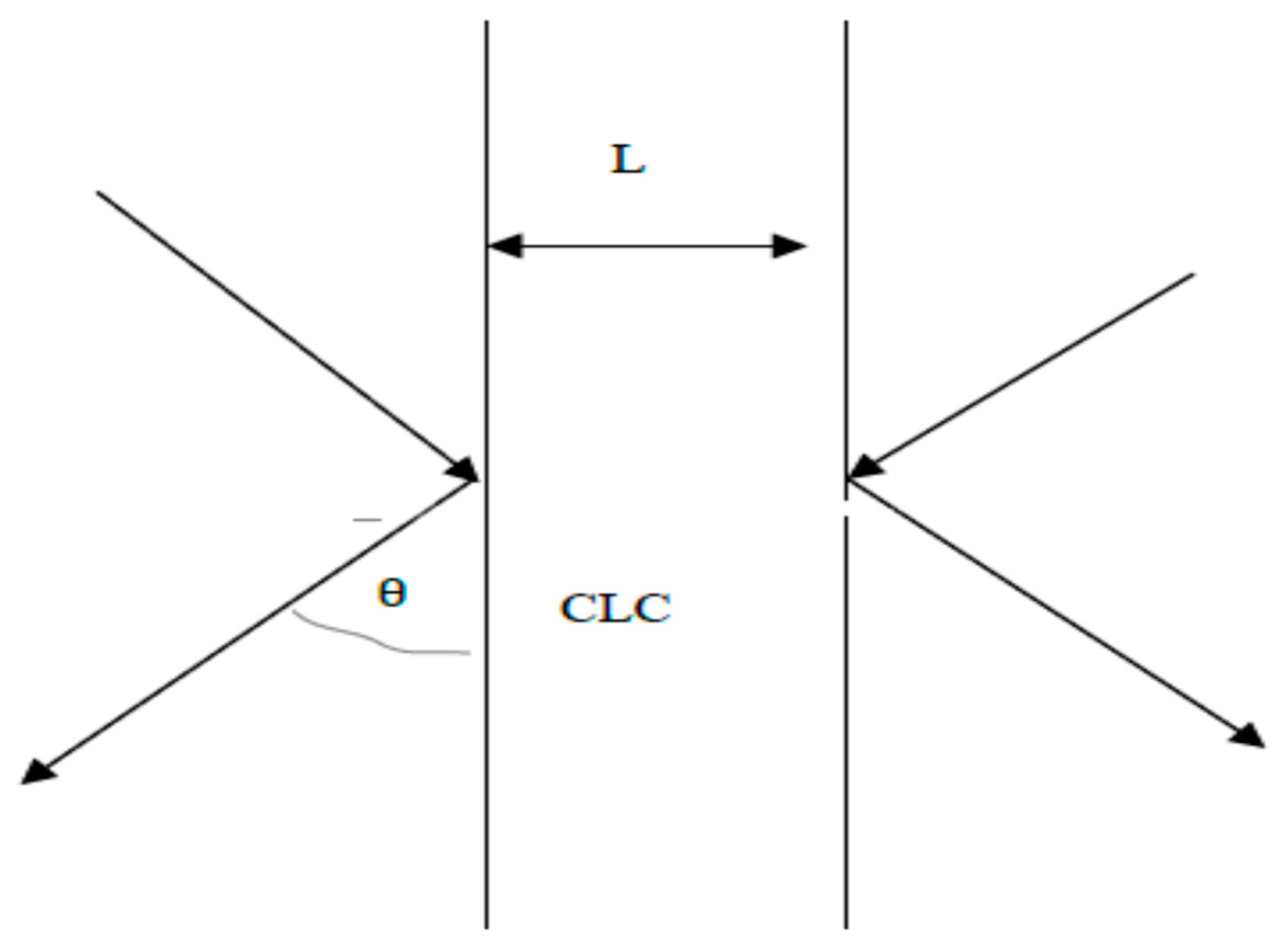
The solution of the system (2) shows [12,13] that for a non-collinear geometry (light propagating at an angle to the CLC helical axis) the Eigen waves polarization vectors change slightly inside the stop band (at variations of the wavelength or the propagation direction). As an approximation for the Eigen waves polarization vectors (neglecting their changes inside the stop band) a kinematic expression may be taken into account for the Eigen polarizations (see [12,13]). As a result of the solution of the system (2) one finds for each Eigen polarization two Eigen waves with different diffraction additions to the wave vectors q^± which are strongly dependent on the deviation of the wave vectors (or the frequency) from the exact Bragg condition. We shell use below an explicit expression for the Eigen waves for the collinear geometry (see, for example [12]) and an approximate expression for the Eigen waves for the non-collinear geometry [13]. Note that, for the non-collinear geometry, the Eigen waves are dependent on the parameter α determining the deviation from the Bragg condition (α = τ(τ + 2k)/k²). Note that the general expression for the parameter reduces to α = 2(Δω/ω_B)sinθ_B for a changing the frequency by Δω at the fixed incidence angle and to α = 2Δθsinθ_B for a changing the the incidence angle by Δθ at the fixed frequency, where ω_B and θ_B are the Bragg frequency and the Bragg angle (see Figure 1), respectively.

For finding the localized edge mode we have to solve a boundary problem for a CLC layer. The case of a collinear geometry corresponding to the edge mode (EM) is well known [12]), so, in the next section, we discuss the case of a non-collinear geometry corresponding to the conical edge mode (CEM).

3. Boundary Problem

Begin by considering the boundary problem in the formulation which assumes that a plane optical wave with diffracting polarization is obliquely incident at the planar CLC layer (see Figure 1). The amplitudes of the two Eigen waves E_±⁺ and E_±⁻ excited in the CLC layer by the incident wave (with the amplitude of incident wave equal to unity and the propagation direction close to the one given by the Bragg condition) are determined by the following equations

E₊⁺ + E₋⁺ = 1
exp[i K^t−₊K^t− + L]ξ⁺E₊⁺ + exp[iK^t− − L]ξ⁻E₋⁺ = 0,

(3)

where L is the layer thickness and K^t−₊ and K^t−₋ are the normal (along the reciprocal vector τ) components of the wave vectors, and ξ^± = (E⁻/E⁺) = P(ε_τ)/(α ± [α² − (P(ε_τ))²]^½).

The amplitude reflection R_a and transmission T_a coefficients for light of diffracting polarization take the form:

R_a = -iP(ε_τ)sinqL/[(4q/τ)cosqL − iαsinqL]
T_a = (4q/τ)exp[iτL/2]/[(4q/τ)cosqL – iαsinqL],

(4)

where for the first diffraction order

q = (τ/4)[(α)² − ((δ/2)(1 + sinθ))²] ^½.

(5)

The intensity reflection R = R_a² and transmission T = T_a² coefficients experience oscillations versus the frequency outside the stop band. In non-absorbing layers the relation R +T = 1 holds for all frequencies. At q = nπ/L, where n is an integer number, R = 0 and T = 1.

4. Conical Edge Modes

There is a complete analogy between the case of a collinear geometry and the case of a non-collinear geometry. Thus, similarly to the well-known CLC localized edge modes (EM) existing at discrete frequencies outside the optical stop band, in the case of a non-collinear geometry, the localized conical edge mode (CEM) should also exist at discrete frequencies outside the stop band. In both cases, collinear and non-collinear geometry, the localized mode frequency is found from the resolvability condition of similar systems of two equations, so there is a qualitative similarity of the results with some quantitative difference.

Similar to the case of collinear geometry studied in [12], the dispersion equation for CEM can be obtained as a condition of resolvability of the homogeneous equation obtained from Equation (3). Note that, as follows from the solution of the homogeneous equation, the CEM is a linear superposition of two Eigen waves with the amplitude ratio E₋⁺/E₊⁺ = −1. The resolvability condition demands a zero value of the Equation (3) determinant and results in the following dispersion equation for CEM:

tg(qL) = −4i(q/τ)/α.

(6)

In a general case the solution of Equation (6) determining the CEM frequencies (ω_CEM) can be found only numerically. The CEM frequencies ω_CEM occur to be complex quantities which may be presented as ω_CEM = ω⁰_CEM(1 + iΔ), where Δ in real situations is a small parameter. So, the CEMs are weakly decaying in time, i.e., they are quasi-stationary modes. Luckily, an analytic solution may be found for some limiting cases, namely, for a sufficiently small ensuring the condition (qL)Im(q/τ) << 1. In this case the values of a real part of ω_CEM, i.e., ω⁰_CEM, are coinciding with the frequencies of zero values of reflection coefficient R for a non-absorbing CLC layer and the complex CEM frequencies are determined by the relations:

(Lq) = nπ, Δ = −(1/2)P(ε_τ)(nπ)²/[(P(ε_τ)Lτ/4]³

(7)

where n is an integer number numerating the CEMs.

The CEM lifetime in this limiting case is proportional to the third power of the sample thickness L, and for the first diffraction order CEM is given by the expression

τ_{CEM ≈} (Lε₀^½/c)[(δ/2)(1+sinθ)Lτ/πn]²

(8)

where c is the speed of light.

The CEM properties are similar to the ones of EM, and their detail description may be found in [13], so below will be mentioned main CEM properties without their detail derivation. The CEM are numerated by an integer number n (n =1 corresponds to the CEM whose frequency is the closest to the stop band edge), the electromagnetic field of CEM is localized in the layer and is modulated in the space at the layer thickness with the number of modulation periods coinciding with the CEM number n. In a non-absorbing CLC layer, a finite CEM lifetime is due to the radiation leakage through the layer surfaces, so the CEM lifetime increases with the increasing of the layer thickness L as a third power of L according to (8), and resulting in an infinite CEM lifetime for the infinite L.

5. Spectral (Angular) Distribution in Kossel Line

Similarly to the X-ray case, the optical Kossel lines are due to the emission of radiation by individual atoms located in a periodic medium (CLC in our case) resulting in an essential angular redistribution of the fluorescence radiation emitted from a sample for the emission directions close to the ones satisfying the Bragg condition. In the case of a planar CLC layer these directions form a circular cone around the normal to the CLC layer surface. There are two typical ways of observing peculiarities of the fluorescence in CLC. One approach consists in measuring the fluorescence spectrum at a fixed emission angle and the other in the measuring of the fluorescence angular distribution close to the Bragg direction at a fixed emission frequency. The experimental curves of angular and frequency dependencies obtained in both approaches are very similar. So, to be specific, we shall discuss below the first option, spectral measurements at a fixed observation angle, keeping in mind that the theoretical description for the second option may be easily obtained by a simple redefinition of the parameters entering in the formulas of the first approach. The experimentally observed peculiarities of the fluorescence in CLC happen for the mentioned above emission directions constituting a circle cone with its axis along the CLC spiral axis (in the case of a planar CLC layer this direction coincides with the direction of the normal to a CLC layer surface). Some fine structures of the intensity distribution for a definitely polarized fluorescence (in the case of the first order of diffraction for the elliptically polarized fluorescence) are observed at this cone.

Beginning by considering the characteristics of the exiting from the sample light (in our case the fluorescence optical Kossel lines (KL)), we note that the emission in a sample radiation propagates according to the rules for the Eigen waves propagation in the sample. This is why the characteristics of exiting from the sample radiation (including the optical KL) are dependent on the properties of the Eigen waves of the sample. One easily finds that in the case of the optical KLs relevant Eigen modes are the CEMs.

In the optical problems corresponding to the boundary problem schematically shown in Figure 1 (just to which relates the considered below problem of light emission by a point source placed in a perfect CLC layer) an equation of the following form should be studied.

RotRot E − c⁻²ε(r)∂² E/∂t² = F(r,t),

(9)

in (9), E is the electric field vector, ε(r) is the dielectric tensor of the CLC layer in Figure 1, and F(r,t) is the vector function whose specific form is determined by the studied physics process. This may be a problem of nonlinear frequency conversion or a problem of emission by a moving charged particle, etc., [12]. A common result of the mentioned specific cases is finding of the Eigen wave amplitudes excited in the layer due to the inhomogeneity F(r) in (9). In the present case, the optical KLs are similar to the ones for X-rays [1,2,3] (light emission by a point source placed in a perfect CLC layer) as an inhomogeneity in (9) should be used the function F(r) corresponding to a point emission source (individual atom) differing from zero only inside the layer. Naturally, in a direct analogy with the X-ray case, the influence on the emission of a periodical medium (CLC) reveals itself in the suppression of the emission in directions corresponding to the stop band (in the case of fixed light frequency) and an essential redistribution in the angular distribution of light close to the directions of the stop band edges (just this redistribution creates the Kossel lines). For the emission angles far from the stop-band directions, the CLC periodicity does not practically influence the light emission. So, there is a fine angular structure of the light emission close to the directions of the stop band edges. Along with the emission suppression for the directions corresponding to the stop band, emission maxima arise at the directions corresponding to the CEMs of the different numbers n out of the stop band directions. This is nevertheless close to the directions corresponding to the stop band edges.

If we first neglect light absorption in the CLC, the CEM amplitudes for a different n may be found from the solution of the system (3). As was shown in [12,13] at the CEM frequencies, determined by the relations

(Lq) = nπ, with q = (τ/2)[(α_p)² − (P(ε_τ))²] ^½,

(10)

the found from the solution of system (3) E₊⁺ and E₋⁺ practically coincide with the corresponding amplitudes of n^th CEM excited in a sample.

For a first diffraction order, an explicit expression in the two-wave dynamical diffraction approximation for the frequencies of CEM with different number n following from (10), and correspondingly the frequency positions of maxima in KL spectrum are determined by the expression

± (ω − ω_B)/ω_B = (1/2)[(1 + sinθ)² (δ/2)² + (np/L)²]^½, n = 1, 2, 3......

(11)

where the Bragg frequency ω_B = (cτ/2ε₀^½)/sinθ.

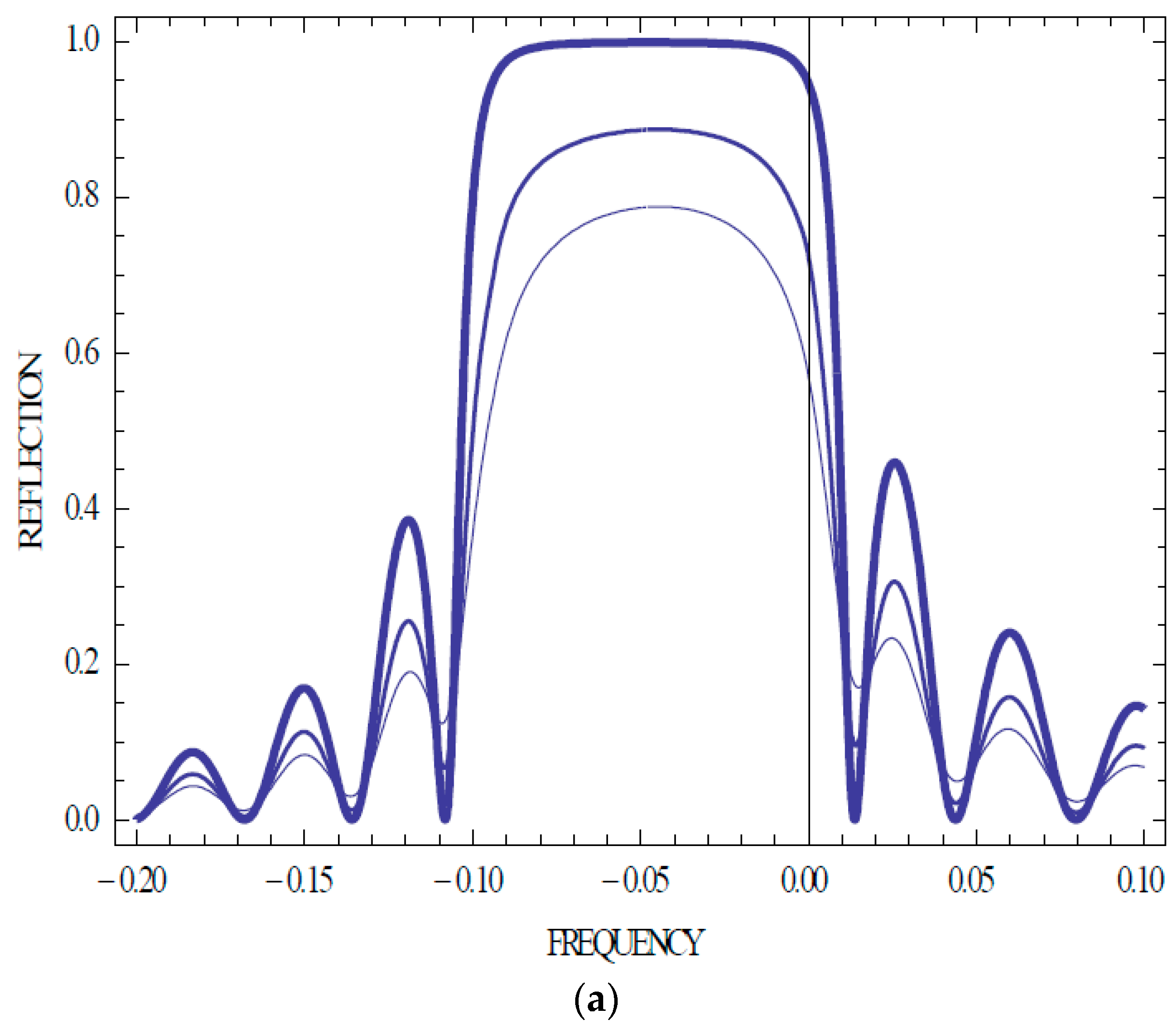
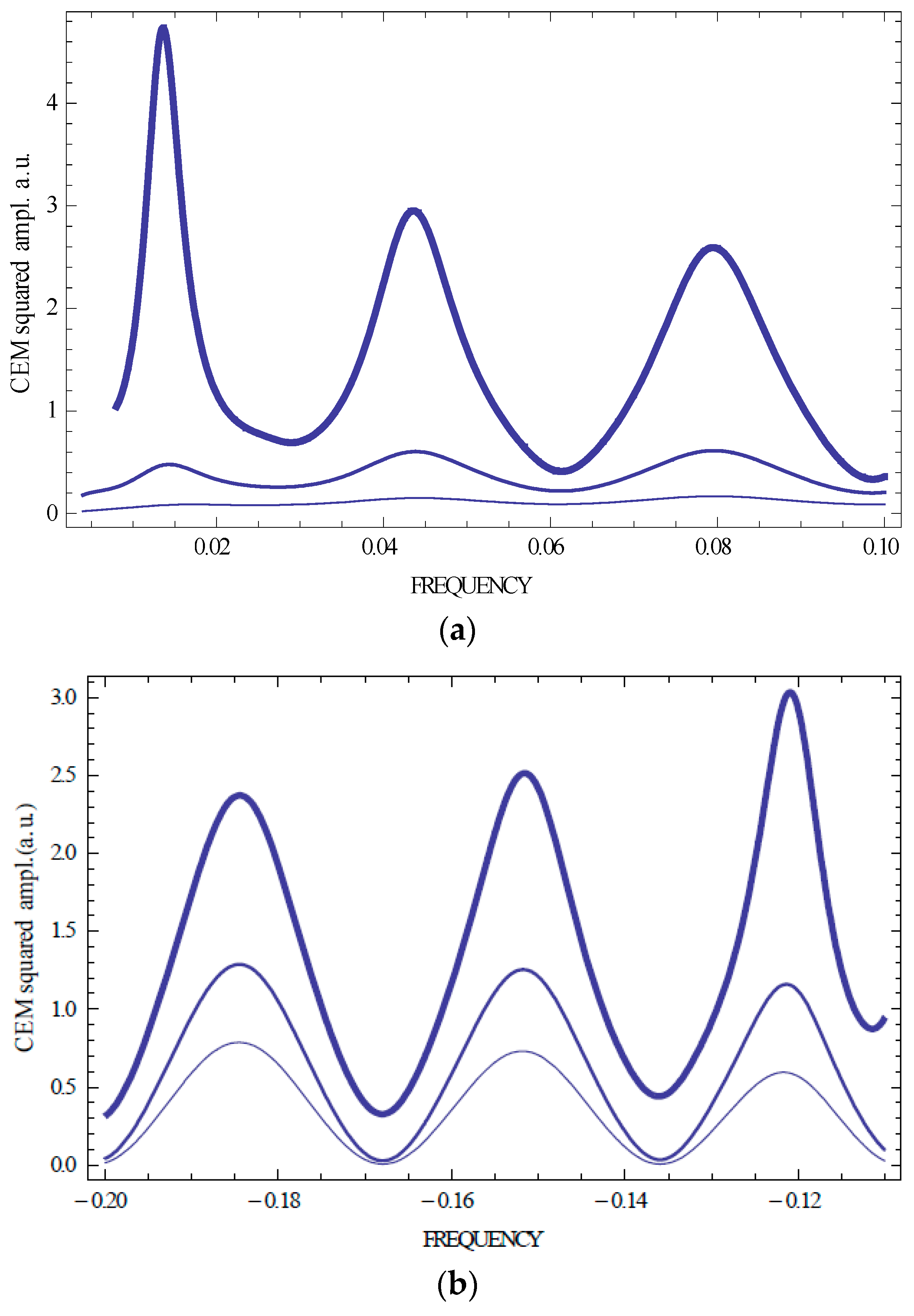
So, there is a fine structure of emission lines determined by the difference in the frequencies of the CEM corresponding to a differing n. Figure 2 and Figure 3 present calculation results for the squared CEM amplitudes for several first CEMs (n = ±1, ±2, ±3) carried out with help of the system (3). One sees that the KL spectrum is symmetric relative to the stop band if a sample is non-absorbing (Figure 2 and Figure 3 show that the spectral location of the CEM amplitude maxima coincide with the locations of the zero values of the reflection coefficient).

Figure 2 and Figure 3 demonstrate also a strong dependence of the spectral positions and intensities of the Kossel lines on the sample thickness.

6. Absorbing CLCs

The above-discussed spectral distribution of the Kossel lines with neglecting of the light absorption has a limited application for describing a real experiment. It may be relevant to very thin samples, while, as a rule, the absorption determines the essential features of the experiment. This is why we will also consider the light absorption in the study of the previous section beginning from the case of an isotropic light absorption. The isotropic absorption may be taken into account by introducing a small imaginary part in the homogeneous part ε₀ of the CLC dielectric tensor, i.e., assuming ε =ε₀(1+iγ) where γ is a small positive parameter. Figure 4 presents the calculation results of the same quantities as in Figure 2 and Figure 3 but for the isotropically absorbing sample.

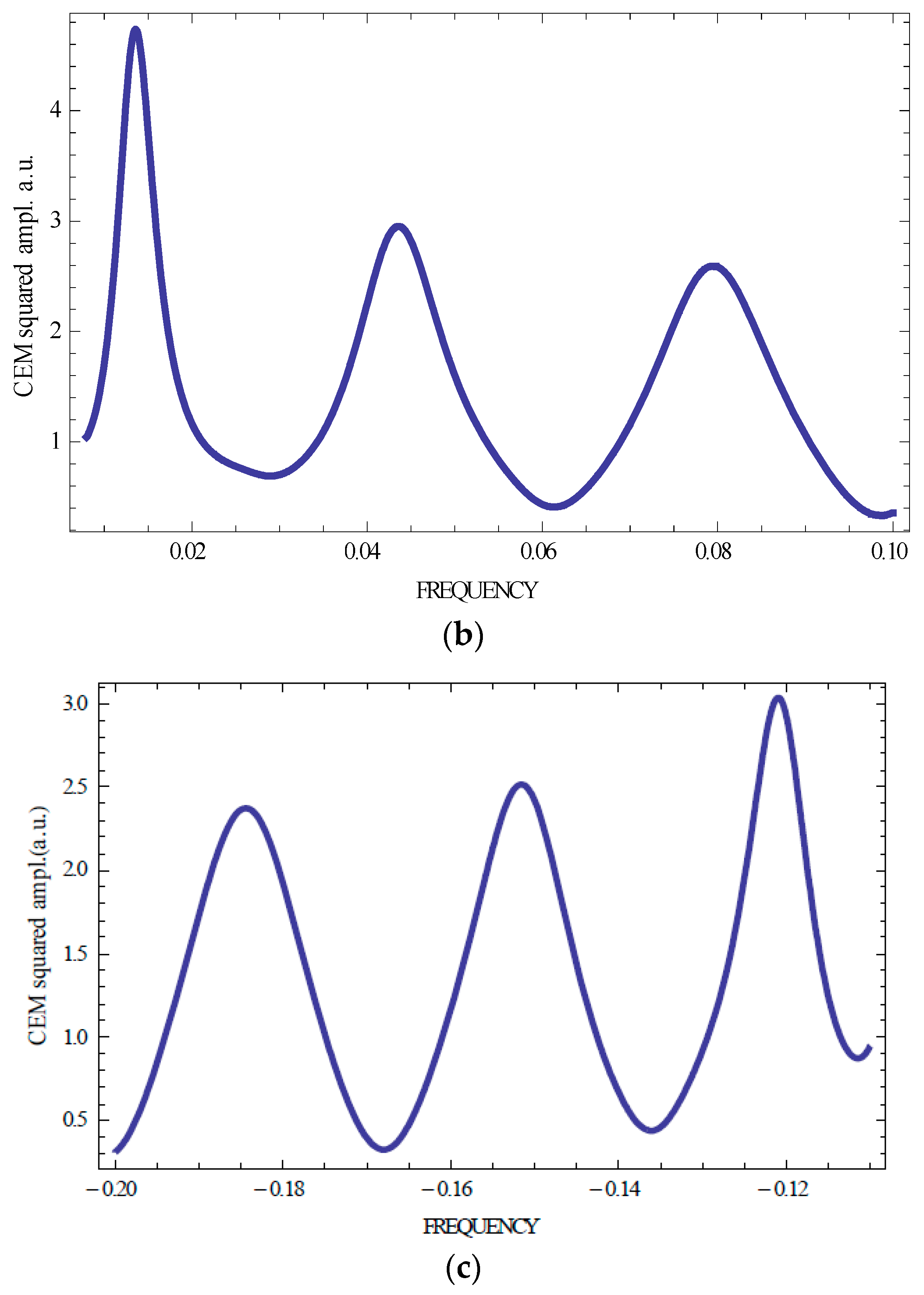
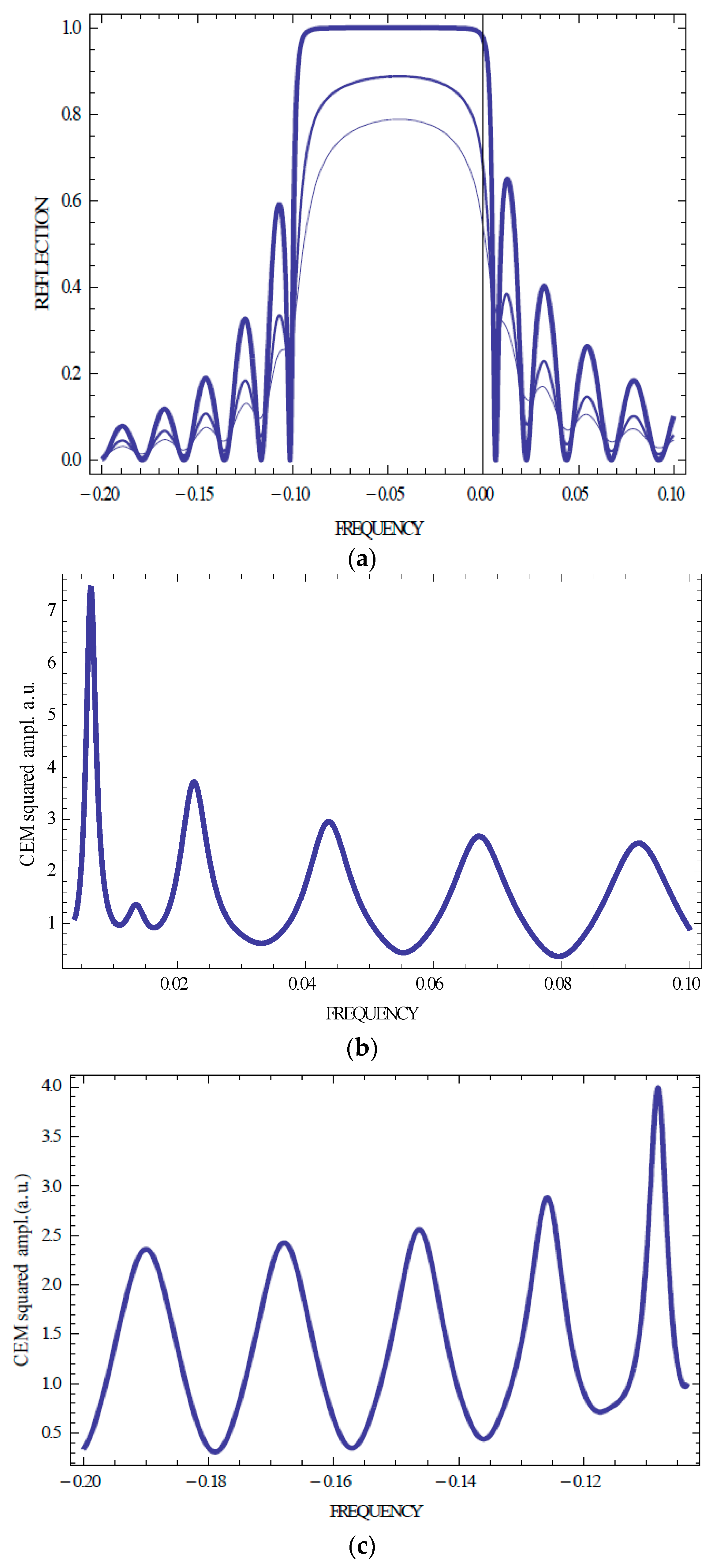
Figure 2, Figure 3 and Figure 4 show that an isotropic absorption does not change the Kossel lines spectral shape and conserves, in particular, the spectrum symmetry relative to the stop band. However, an isotropic absorption decreases the EM amplitudes for all numbers n. Sometimes, the amplitudes corresponding to the higher n are larger than the amplitudes corresponding to lower n (see Figure 4 showing that the largest amplitude corresponds n equal 1 or 2 for different strength of the absorption). This is a manifestation of the anomalously strong absorption effect [12]. Note that for absorbing samples in contrast to non-absorbing ones, the reflection coefficient R in its frequency beats does not reach zero value at its minima (see Figure 2a and Figure 3a). In the case of an isotropically absorbing CLC, the intensity of the emitted from a sample radiation, related to one event of the emission, is reduced compared to the case of the non-absorbing CLC. Dependence of the Kossel lines spectrum on the layer thickness can be seen from a comparison of Figure 2 and Figure 4 with Figure 3 for a changed sample thickness.

7. KL Spectrum Influenced by the Borrmann Effect

It is known that, in perfect absorbing CLC layers the diffraction process may be strongly influenced by the Borrmann effect. The Borrmann effect was firstly discovered in the X-ray diffraction and later was observed in the photonic liquid crystals (see, for example, [12]). The Borrmann effect in CLC is due to the local absorption anisotropy of CLC and under the diffraction conditions results in an enhancement of the light beam for some its propagation direction close to the one stop band edge. In contrast, the other propagation direction close to the other stop band edge results in a suppression of the beam in a narrow angular range. In other words, the Borrmann effect reveals itself by decreasing or increasing of the light absorption in perfect absorbing CLC samples. Naturally, the Borrmann effect influences the Kossel line spectra in the X-ray case [2,3] so for the fluorescence in CLCs it should be present in an optical wave-length range. As will be shown below, the influence of the Borrmann effect on the Kossel line spectra in CLC is naturally described in the frame work of the approach proposed in the present paper for the optical Kossel lines.

The Borrmann effect in CLCs, as was mentioned above, is due to the existing of a local absorption anisotropy in CLCs and was observed in optical reflection and transmission spectra (see, for example [12,14]), meanwhile, as will be shown below, it reveals itself also in the fluorescence spectra of perfect photonic liquid crystals. Currently, there are number of papers where peculiarities of the fluorescence in CLCs were studied (for example [5,6,7,8,9,10,11]). In the cited papers, peculiarities of the fluorescence spectra, angular distribution and polarization properties were observed for the definite directions of the fluorescence emission in CLCs.

We shall illustrate below the manifestation of the Borrmann effect for a collinear diffraction geometry because most experimental studies of the Borrmann effect were performed just for this geometry. In this case, the Kossel cone degenerates in one point (one direction) and correspondingly the CEM converts in its limiting case, the EM, and the Borrmann effect exists for a diffracting circular polarization, right or left, in accordance with the CLC spirality.

The frequencies of EM with different number n, and correspondingly the frequency positions of maxima in KL spectrum for a collinear geometry are determined by the expression (see [12]) similar to (11):

±(ω − ω_B)/ω_B = (δ/2)[1 + (np/δL)²/2], n = 1, 2, 3……

(12)

where the Bragg frequency ω_B = cτ/2ε₀^½.

As previously shown [12], the Borrmann effect in photonic liquid crystals is strongly influenced by the temperature. This temperature influence reveals itself via the order parameter S of the dye molecules. For S = 1 this influence, resulting in a Kossel spectrum asymmetry, is strongest and becomes weaker with the decreasing of S, and at S = 0 the Borrmann effect disappears while a restoration of the Kossel spectrum symmetry happens.

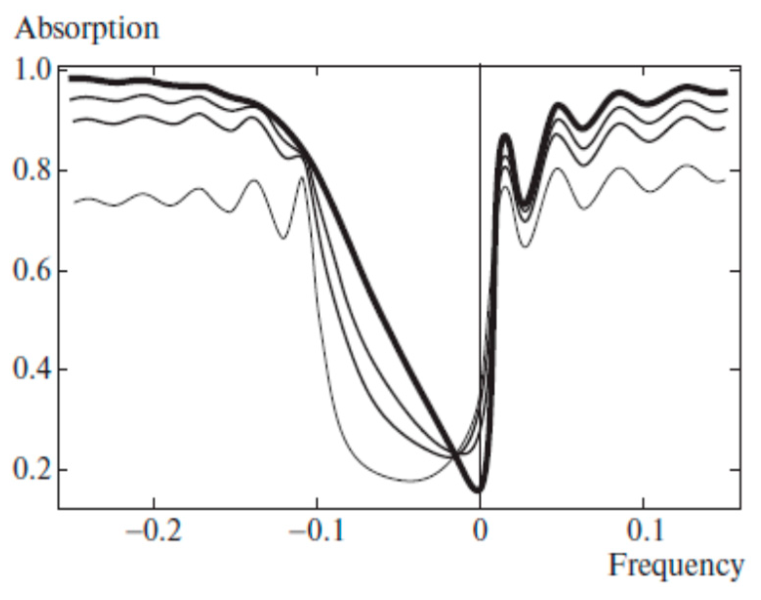
As an illustration of the absorption spectrum asymmetry due to the Borrmann effect and its dependence on the order parameter S, the calculation results are presented in Figure 5 and Figure 6.

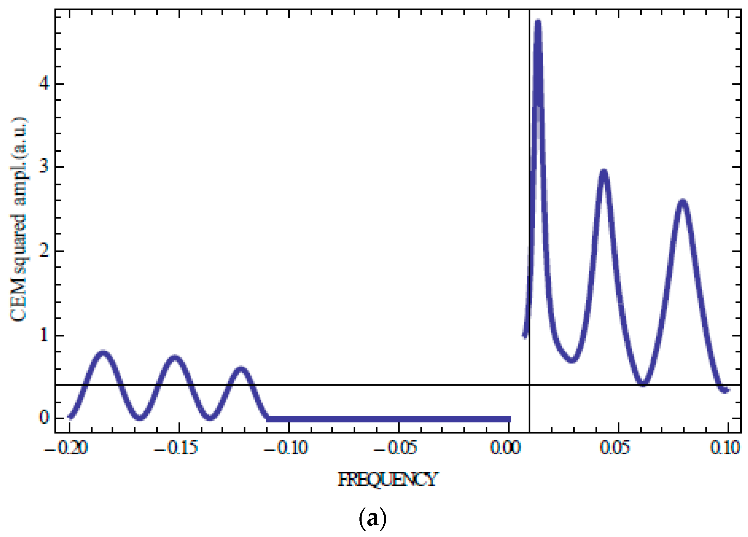
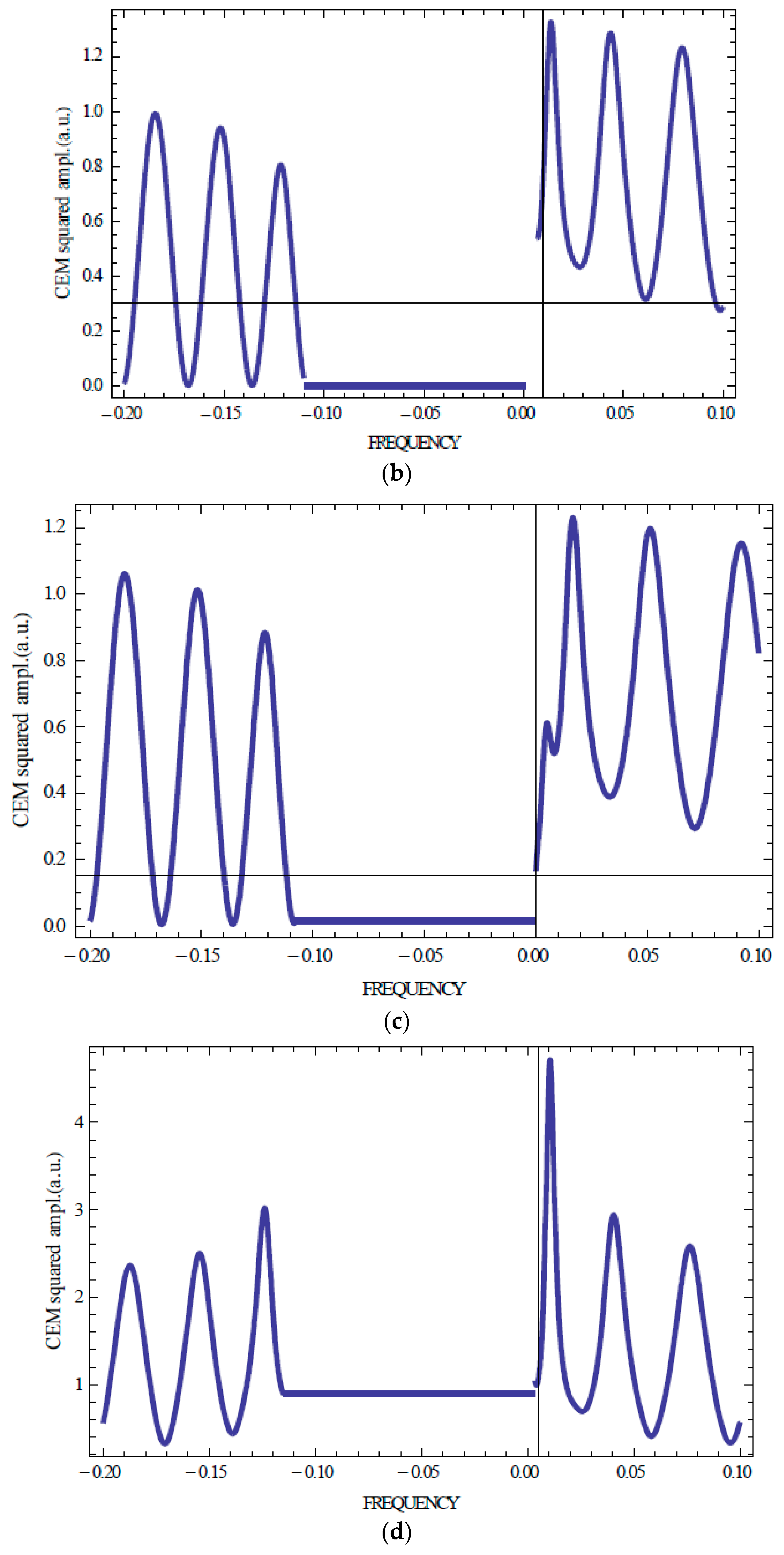
Figure 6 presents KL fluorescence spectra of a perfect CLC layer for light with diffracting circular polarization at various values of the order parameter S.

Figure 6 shows the Borrmann effect results in a growth of the Kossel lines amplitudes at the high-frequency stop band edge and their decrease at the low-frequency stop band edge compared to the case of isotropic absorption (S = 0) with a maximal effect at S = 1 which is in a complete agreement with Figure 5 demonstrating the absorption suppression at the high-frequency stop band edge. Note that in the calculations presented in Figure 6 the expressions for the CLC dielectric tensor principal values ε_// and ε_⊥ assume that the absorbing oscillator axis in the dye molecule is parallel to the long molecular axis.

In the case of CEM (non-collinear geometry) the Kossel line spectra (situated now at a circular cone of light propagation directions with its axis coinciding with the CLC helical axis) are qualitatively similar to the case of a collinear geometry. However, there is an essential difference in the polarization properties of the fluorescence spectra. In this case, peculiarities of the fluorescence are revealed by light with elliptical polarization which deviation from the circular one becomes larger with the increasing of the deviation of light propagation direction from the CLC helical axis (see [13]).

For an analytic theoretical description, due to the higher diffraction orders (in reality, the second one is most essential) the case of KLs is simpler and is presented in the next section.

8. KLs Due to the Second Order Diffraction in CLC

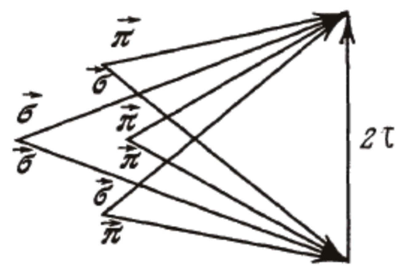
It follows from the paper [14], where CEMs of higher diffraction orders were studied, that the polarization properties of the KLs of the second diffraction order are simpler than the ones of the first diffraction order. In this case, the peculiarities of fluorescence are revealed by light with linear π− and σ− polarizations. The KL cone in this case splits into four cones with slightly differing emission directions. The mentioned splitting shows Figure 7 presenting the second order Bragg conditions in vector form for a CLC and shows that four KL cones are formed by a rotation of the shown wave vectors around the CLC reciprocal lattice vector τ (it is assumed that τ is normal to the CLC layer surface).

Obtaining the Eigen waves and solving of the boundary problem for the second diffraction order in the two-waves dynamical diffraction approximation are very similar to the first diffraction order case studied above. Luckily, the corresponding equations in the case of the second diffraction order are simpler [15]. In Equation (1) for the Eigen waves the polarization vectors σ₊ and σ₋ correspond to the linear π- and σ- polarizations (the conventional definition assumes that the linear π- polarization lies in the scattering plane and the linear σ- polarization is perpendicular to the scattering plane). The systems of two equations for the vector amplitudes (2) and (3) in the case of the second diffraction order are reducible to four independent pairs of equations for scalar amplitudes corresponding to the four combinations of the linear π- and σ- polarizations shown in Figure 7. The corresponding pairs of equations differ only in the explicit expressions for the P(ε_τ) and P(ε_-τ) entering in (2) [15] which are given by the following relations (different from the ones for the first diffraction order)

κ_q = (ω/c)(ε_q)^1/2, ε_π = ε₀ [1 − δ(cosθ)/2], ε_σ = ε₀ [1 + δ(cosθ)/2]
F_πσ = F_σπ = δ²(cos²θ)/4sinθ; F_ππ = δ²(cos²θ)/4, F_σσ = δ²(ctg²θ)/4

(13)

So, the fluorescence polarization in the neighboring KL cones changes between linear π− and σ− polarizations corresponding to the linear π− polarizations for the cone with smallest apex angle.

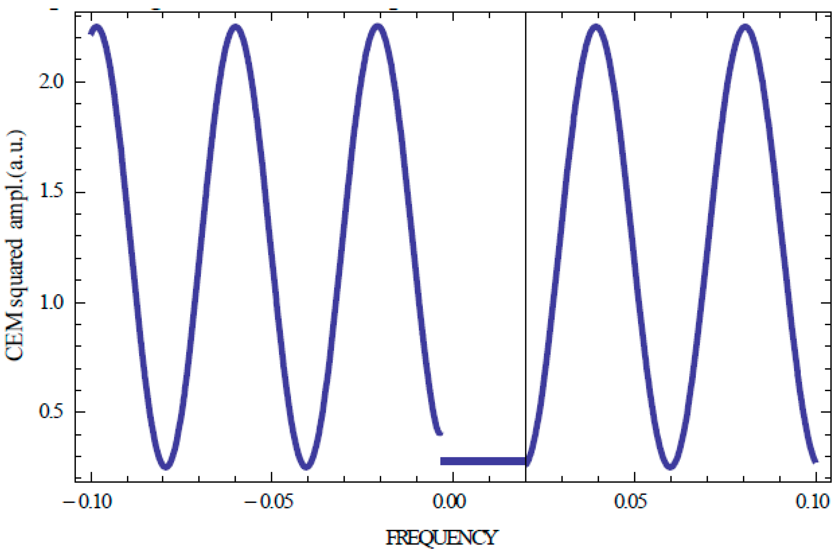
The frequency intervals between the neighboring fluorescence intensity maxima (differing by one in the number n) in an individual KL cone are much larger than in the case of the first diffraction order because, in the case of the second diffraction order, a small parameter of the theory is proportional to δ² (see (13)) while for the first diffraction order it is proportional to δ. For the same reason (smaller value of the small parameter), for a distinct observation of the KL cones of the second diffraction order one needs to have thicker perfect CLC layers than in the case of the first diffraction order. Layers which are sufficiently thick for the first diffraction order might be insufficiently thick for the second diffraction order for demonstrating in an optimal regime the influence of diffraction on the fluorescence. For example, Figure 8 shows that for the same as for the first diffraction order CLC layer thickness the frequency intervals between the consequent CEM frequencies are larger than the frequency width of the second diffraction order stop band. The last statement means that that the second order diffraction effects for a CLC layer of a such thickness would be weak.

9. Discussion

The study carried out above of the peculiarities of fluorescence in CLC due to light diffraction at the CLC periodic structure allows us to describe in a single approach (optical localized edge modes) all experimentally observed features of the fluorescence in CLCs and gives an analytic method to calculate the measurements results, related to the mentioned fluorescence peculiarities (optical Kossel lines) for any specific experiment. The proposed approach describes the fluorescence peculiarities in CLC, related to the angular, spectral fluorescence distribution, its unusual polarization properties, related to the influence on the fluorescence of the light absorption in CLCs, and to the Borrmann effect manifestation in fluorescence. However, there is an item which is out of the performed study scope. This is a calculation of the absolute intensity of the fluorescence exiting a CLC layer at KLs. In an experiment, the observed fluorescence intensity is a result of incoherent summation of many atomic emission acts happening at different locations in a CLC layer. Above, we studied the emission of CEM existing in a CLC layer. In our approach, the fluorescence KL in a CLC layer originates as a result of the CEM decay (emission). It is evident that to calculate an absolute intensity one needs to know how the probability of the CEM excitation in an individual emission act depends on the emitting atom locations in a CLC layer. Naturally, we believe that the CEM excitation probability by an atomic emission act close to the CLC layer surface and in the middle of a CLC layer are different. So, we presented above intensity of fluorescence exiting a CLC layer at KLs in arbitrary units because the corresponding distribution differs from the absolute intensity distribution only by a some factor due to the fact that the absolute intensity distribution is a sum of the CEM distributions multiplied by the corresponding to the emitter location probability factor.

Note that the KL spectra are calculated in the assumption that the Eigen fluorescence spectra (spectra in a homogeneous liquid) are flat. Taking into account of the Eigen fluorescence frequency dependence has to change slightly the curves presented in some figures. A way to exclude the Eigen fluorescence frequency dependence was applied in paper [6]. It was reached by dividing the observed fluorescence intensity with diffracting polarization at the fluorescence intensity with non-diffracting polarization. The spectral curves obtained by this method in [6] fit very well our calculations (see Figure 6) which assume that the Eigen fluorescence spectra are flat. In particular, this is true for the flat parts of the curves inside the stop band obtained in [6] by the above-mentioned procedure.

Concerning the experimental studies of fluorescence for the directions differing from the direction of the CLC helix, they are presented in papers [7,10]. In both cited papers it was observed that the fluorescence polarization forming KL (experiencing diffraction influence) differs from the circular one. The authors of [10] also reported on the observation of the Borrmann effect. Namely, an asymmetry of KL spectra relative to the stop band was observed for the dissolved in CLC dye molecules with the order parameter S > 0 while for S = 0 the observed spectra were symmetric, which also follows from our calculation results presented above in Figure 6. Another example of an agreement of the theory and the experiment is given by the observation in [7] of the second diffraction order fluorescence KL. The measurements performed in [7] show that the fluorescence polarizations in a second diffraction order KL cones are linear ones and are mutually orthogonal for the neighboring KL cones, which is in complete agreement with the study of the second diffraction order KL presented above in Section 8. However, in [7] only three fluorescence second diffraction order KL cones were resolved instead the four ones predicted by the theory. This may be due to a high level of noise in the corresponding measurements mentioned by the authors of paper [7].

10. Conclusions

As a result of the present study one has a clear physical picture of the fluorescence peculiarities in CLC which are due to the CEMs existing in perfect CLC layers. Concerning the fluorescence polarization properties in KLs, they are determined by the CEMs polarization properties and the fluorescence intensity maxima positions in KL spectra coincide with the consequent CEMs frequencies for different n numerating the CEMs. At a negligible small absorption in a CLC layer the KL spectra are symmetric relative the stop band edges while at a sufficiently strong absorption this symmetry might be broken due to the Borrmann effect. As a result of the performed study the following general, not evident, statement may be formulated. The Kossel lines intensity in an absorbing CLC for an individual emission event decreases with the sample thickness increase; however, this decrease can be absent (or reduced) at the fluorescence frequency subject to realization of the Borrmann effect.

Note that a direct connection of the KLs with the CEMs might be proved by means of a time-delayed technique. If after light emission by an individual atom a formation of the fluorescence KLs proceeds via a CEM excitation, the emission of a fluorescence photon from a CLC layer will be delayed relative to the time of an individual atom emission act by a time interval determined by the CEM lifetime (see (8)). For a sufficiently thick and perfect CLC layer, the corresponding time delay might exceed the time of a fluorescence photon emission by an individual atom. So, the observation of a time delay in the fluorescence KLs might be regarded as a direct prove of the physical mechanism of the fluorescence in KLs origin as the one proceeding via CEM excitation.

Note also that the influence of a CLC periodic structure on the Cherenkov radiation in a CLC is similar to the one in the case of fluorescence in a CLC and, compared to the case of a homogeneous liquid, the additional diffraction Cherenkov cone in CLC (see Chpt.9 in [12]) is very similar to the fluorescence KLs studied above. Finally, it should be mentioned that the fluorescence KLs structure in Blue Phases (BPs) is very similar to the X-rays KLs because in the BP case the fluorescence KL cones are formed around different directions, as it happens in conventional crystals in the X-ray case (it was experimentally observed for BPs, see, for example [16,17,18]), in contrast to the CLC case, where all fluorescence KL cones are formed around the CLC spiral axis.

References

- Kossel, W.; Loeck, V.; Voges, H.Z. Die Richtungsverteilung der in einem Kristall entstandenen charakteristischen Röntgenstrahlung. Z. Phys. 1935, 94, 139–144. [Google Scholar] [CrossRef]
- Cowley, J.M. Chapter 1-Fresnel and Fraunhofer Diffraction. In Diffraction Physics, 3rd ed.; Elsevier: North-Holland, Amsterdam, 1995. [Google Scholar]
- Authier, A. Dynamical Theory of X-Ray Diffraction; Oxford University Press: Oxford, UK, 2001. [Google Scholar]
- Belyakov, V.A. Proceedings of the XXIV International Symposium Nanophysics and Nanoelectronics. Available online: http://nanosymp.ru/en/index (accessed on 23 June 2020).
- Nishkawa, S.; Kikuchi, S. Diffraction of cathode rays by mica. Nature 1928, 121, 1019–1020. [Google Scholar] [CrossRef]
- Schmidtke, J.; Stille, W. Fluorescence of a dye-doped cholesteric liquid crystal film in the region of the stop band: Theory and experiment. Eur. Phys. J. 2003, 31, 179–194. [Google Scholar] [CrossRef]
- Risse, A.M.; Schmidtke, J. Angular-dependent spontaneous emission in cholesteric liquid-crystal films. J. Phys. Chem. C 2019, 123, 2428–2440. [Google Scholar] [CrossRef]
- Wang, Z.; Yang, C.; Li, W.; Chen, L.; Wang, W.; Cai, Z. Dye-concentration-dependent lasing behaviors and spectral characteristics of cholesteric liquid crystals. Appl. Phys. B 2013, 115, 483–489. [Google Scholar] [CrossRef]
- Dolganov, P.V. Luminescence spectra of a cholesteric photonic crystal. JETP Lett. 2017, 105, 657–660. [Google Scholar] [CrossRef]
- Penninck, L.; Beeckman, J.; de Visschere, P.; Neyts, K. Light emission from dye-doped cholesteric liquid crystals at oblique angles: Simulation and experiment. Phys. Rev. E 2012, 85, 041702. [Google Scholar] [CrossRef] [PubMed] [Green Version]
- Umanskii, B.A.; Blinov, L.M.; Palto, S.P. Angular dependences of the luminescence and density of photon states in a chiral liquid crystal. Quantum Electron. 2013, 43, 1078–1081. [Google Scholar] [CrossRef]
- Belyakov, V.A. Diffraction Optics of Complex Structured Periodic Media, 2nd ed.; Springer: Berlin/Heidelberg, Germany, 2019. [Google Scholar]
- Belyakov, V.A. Localized conical edge modes in optics of spiral media (first diffraction order). Crystals 2019, 9, 674. [Google Scholar] [CrossRef] [Green Version]
- Aronishidze, S.N.; Dmitrienko, V.E.; Khoshtariya, D.G.; Chilaya, G.S. Recent developments in gauge theories. Pis’ma ZhETF 1980, 32, 19. [Google Scholar]
- Belyakov, V.A.; Semenov, S.V. Localized conical edge modes of higher orders in photonic liquid crystals. Crystals 2019, 9, 542. [Google Scholar] [CrossRef] [Green Version]
- Miller, R.J.; Gleeson, H.F. Rhapsody in blue. Phys. Rev. E 1995, 52, 501–503. [Google Scholar] [CrossRef] [Green Version]
- Otón, E.; Netter, E.; Doi-Katayama, Y. Monodomain blue phase liquid crystal layers for phase modulation. Sci. Rep. 2017, 7, 44575. [Google Scholar] [CrossRef] [PubMed] [Green Version]
- Oton, E.; Morawwiak, P.; Galadyk, K.; Oton, J.M.; Piecek, W. Fast self-assembly of macroscopic blue phase 3D photonic crystals. Opt. Express 2020, 28, 18202–18211. [Google Scholar] [CrossRef]
Figure 1.
Schematic of a boundary problem for the localized conical edge mode (CEM).
Figure 2.
Calculated versus frequency reflection coefficient (a) for non-absorbing and isotropically absorbing CLC layer [δ(1 + sinθ)/2 = 0.05, thickness in period number N = 100, γ = 0, 0.003, 0.006 (shown at decreasing line thickness)], and squared CEM amplitude for a non-absorbing CLC at the high frequency (b) and low frequency (c) stop band edge for three first CEMs (n = ±1, ±2, ±3); here and at all figures below the dimensionless frequency ωd = δ(1 + sinθ)/2[2(ω − ωB)/ωBδ(1 + sinθ)/2 − 1)], where ωB = cτ/2sinθε0½ is used (i.e., normalized by the Bragg frequency the difference of the frequency and the stop band edge frequency).
Figure 3.
(a–c) The same as Figure 2 for the CLC layer thickness in period number N = 150.
Figure 4.
Calculated squared CEM amplitude for non-absorbing and isotropically absorbing CLC layer [δ(1 + sinθ)/2 = 0.05, thickness in period number N = 100, γ = 0, 0.003, 0.006 (shown at decreasing line thickness)], at the high frequency (a) and low frequency (b) stop band edge for three first CEMs (n = ±1, ±2, ±3).
Figure 5.
Absorption of light with diffracting circular polarization for a CLC layer with local anisotropy of absorption versus the frequency for S = 0, 0.3, 0.5, 1 (the curve thickness is growing with an increase in S) at Im[ϵ1]/Re[ϵ0] = 0.03, δ = 0.05, N = 50.
Figure 6.
Calculated Kossel line spectrum of light with diffracting circular polarization for an absorbing sample influenced by the Borrmann effect at S = 1 (a), at S = 0.5 (b), at S = 0.3 (c), at S = 0 (d) (N = 100, δ = 0.05, with the following dependence of the dielectric tensor principal values on S: Im[ε//] = Im[ε1](1 + 2S)/3, Im[ε⊥] = Im[ε1](1 − S)/3, where Im[ε1] = 0.009 is the only non-zero imaginary part in a single principal value at S = 1 [12]).
Figure 7.
Second order Bragg conditions in vector form for a CLC with a strong local birefringence (polarization symbols π and σ at the wave vectors show Eigen waves polarizations related to the corresponding propagation direction).
Figure 8.
Calculated fluorescence Kossel line spectrum of the second order diffraction at θ = 60° and δ = 0.058 for the cone with π− (π−) linear polarizations of light (non-absorbing sample, N = 100, the accepted in Figure 2, Figure 3 and Figure 4 [δ(1 + sinθ)/2 = 0.05 in the second diffraction order. existing at θ = 60o, results in δ = 0.058).
© 2020 by the author. Licensee MDPI, Basel, Switzerland. This article is an open access article distributed under the terms and conditions of the Creative Commons Attribution (CC BY) license (http://creativecommons.org/licenses/by/4.0/).
Share and Cite
MDPI and ACS Style
Belyakov, V.A. Optical Kossel Lines and Fluorescence in Photonic Liquid Crystals. Crystals 2020, 10, 541. https://doi.org/10.3390/cryst10060541
AMA Style
Belyakov VA. Optical Kossel Lines and Fluorescence in Photonic Liquid Crystals. Crystals. 2020; 10(6):541. https://doi.org/10.3390/cryst10060541
Chicago/Turabian StyleBelyakov, Vladimir A. 2020. "Optical Kossel Lines and Fluorescence in Photonic Liquid Crystals" Crystals 10, no. 6: 541. https://doi.org/10.3390/cryst10060541
Note that from the first issue of 2016, this journal uses article numbers instead of page numbers. See further details here.