Article

Numerical Assessment of Flow Pulsation Effects on Reactant Conversion in Automotive Monolithic Reactors

by
Pratheeba Chanda Nagarajan
1,
Henrik Ström
2,* and
Jonas Sjöblom
1
1
Division of Combustion and Propulsion Systems, Department of Mechanics and Maritime Sciences, Chalmers University of Technology, SE-412 96 Gothenburg, Sweden
2
Division of Fluid Dynamics, Department of Mechanics and Maritime Sciences, Chalmers University of Technology, SE-412 96 Gothenburg, Sweden
*
Author to whom correspondence should be addressed.
Catalysts 2022, 12(6), 613; https://doi.org/10.3390/catal12060613
Submission received: 12 May 2022 / Revised: 30 May 2022 / Accepted: 1 June 2022 / Published: 3 June 2022
(This article belongs to the Special Issue Catalysts: Reactor Modeling Using Computational Fluid Dynamics)

Abstract

:
Highly transient engine-out emissions imply significant challenges for the optimization and control of automotive aftertreatment systems, motivating studies of the effects of flow pulsations on the system behavior. In this work, an axisymmetric aftertreatment system with a first-order reaction in the monolith section is chosen to demonstrate the role of pulsations on the time-averaged conversion at the exit. Reactive computational fluid dynamics simulations under transient conditions are performed by applying the SST k- ω turbulence model along with a reactant species balance equation and a porous medium description of the catalyst. Four different types of temporal velocity variations (constant, step-like, sawtooth and sinusoidal) are applied at the inlet. Additionally, the corresponding fluctuations driven by a prescribed inlet pressure are also investigated. It was found that the fluctuations in the incoming flow affect the transient response of the monolith, the time-averaged conversion, the evolution of the flow uniformity index and the dispersion downstream of the catalyst. It is also shown that the retention time distribution is modulated by the pulsations and that the mixed-cup conversion span is different for geometrically identical systems having the same velocity span if the fluctuation characteristics are different. In conclusion, simulations of phenomena that depend on time-resolved boundary conditions from experiments require proper characterization of fluctuations present in the real-world systems; otherwise, the method of recreating the signal at the boundary may influence the obtained results.

1. Introduction

1.1. Background

In-cylinder conditions and combustion of fuels are the basis of harmful automotive emissions. These emissions, even at low but significant concentrations, affect human life and the environment. Catalytic converters are devices of paramount significance, as they are crucial in treating harmful engine-out emissions. Perpetual and significant research advances are very common to match emission levels at the tail pipe prescribed by emission legislations. Stringent legislations promote these enhancements in research. Monolithic catalytic converters are multi-channel devices, with porous catalytic walls [1]. The transport processes and reactive processes that take place in these devices span multitude of timescales and length scales [2]. Owing to such timescales that span from milliseconds to seconds, often simplified models are used to predict the concentration of gases at the outlet of the catalyst.
The performance of catalytic converters are influenced by many factors, for example, the upstream engine-out conditions, the geometry of the catalytic converter cones, the positioning of the catalytic converter after the engine and the flow distribution upstream of the catalytic converter [3]. These factors are incorporated in modeling catalytic converters. These models are of varying complexity, ranging from simplified models to complex three-dimensional models.
One geometrically simple, yet efficient, model is the Single Channel Model (SCM). The SCM assumes that every channel experiences the same flow, temperature and gas concentrations. Of the many assumptions, the flow is assumed to be unidirectional with uniform gas distributions at the inlet despite a three-dimensional geometry and other possible flow disturbances [4]. This assumption of uniform distribution, does not hold as the washcoating in monoliths influences the conversion via the mass-transfer effects [5]. Chakravarthy et al. [6] modeled flow in catalytic and non-catalytic regions under transient conditions. They showed that for practical applications, a detailed characterization of the flow and mixing before the catalyst is required along with heat losses.
Bella et al. [7] studied the effect of flow distortion at the inlet of a catalytic converter on the conversion efficiency of carbon monoxide and hydrocarbon oxidation. They found that the flow distribution led to non uniform utilization of the catalyst. Zygourakis used three inlet velocity distributions (flat, parabolic and pinwheel specifications) [8], with a two-dimensional geometry considering carbon monoxide oxidation kinetics. The conversion of CO was significantly affected by the inlet velocity distribution. Bressler et al. [9] studied the effects of pulsating flow in close-coupled (CC) catalytic converters by experiments and CFD simulations. They found that pulsations influenced mixing in the monolith prechamber and uniform flow improved the ageing and pressure losses in the monolith. Liu et al. [10] performed experiments with sinusoidal inlet pulses, with the aim to study the effect of pulsations on flow uniformity in non-reactive flows and compared them against simulation results. They found that higher frequency pulsations improved the flow uniformity. Similar results were demonstrated with steady-state experiments [11]. Jeong [12] used pulsating input from the engine with constant concentration of gases and showed that periodic dips were experienced in the conversion of reactant gases and that the pulsations affected the local hotspots in the monolith.
It is thus clear that proper characterization of the fluctuations at the inlet of the catalytic converter is crucial to optimise its performance. Experiments face challenges as the frequency of these fluctuations poses a limitation on the instrumentation that can measure the fluctuating quantities under reactive conditions. The pulsations produce changes in mass flowrate and therefore the residence times and hence affect the conversion at the exit. Computational fluid dynamics (CFD) simulations offer advantages in explaining how such fluctuations interact with the geometry to create spatio-temporal effects inside the system. The engine-out flows are transient and turbulent in nature due to changes in load coupled with the driver behavior. The placement of a catalyst near the engine (close-coupled) or far away from the engine (underbody) will also reflect differently on the pulsations that arrive at the inlet. To utilize the temperature of the hot engine-out gases and to speed up the warming of catalyst, it would be advantageous to place the close-coupled converter close to the engine. This placement is achieved by short pipes to the engine, the length of these short pipes would not provide enough residence time for the pulsations from the engine to dampen out [13]. Quantification of pulsations is also important for control purposes. At the same time, CFD simulations offer opportunities for detailed insight into the functionality and optimisation of real-world reactors. For such simulations to be useful, they should however accurately also reflect the real-world fluctuations in the incoming boundary conditions.
Therefore, this work attempts to quantify the effect of pulsations at the inlet on the efficiency of conversion of reactants using transient CFD simulations. To this end, three different inlet velocity distributions are compared against a uniform velocity specification. The inlet boundary condition is specified either as a velocity or as a driving pressure, to investigate the different behaviors provoked by these complementary methods of specifying the flowrate. The main aim of the work is to demonstrate the effect of pulsation characteristics on the time-averaged conversion at the system exit.
The paper is organized as follows: we first present the theory of the timescales involved in after-treatment systems and develop a methodology for analysing the time-averaged conversion and the flow uniformity, by choosing pulsating frequencies such that effect of pulsations are amplified. This section is followed by the geometry and mesh details that are used in the simulation. Then, the mathematical description of the model and the solution methodology are presented. The results are analyzed focusing on the time-averaged conversion and the flow uniformity attained.

1.2. Theory

Table 1 lists the most relevant time scales in automotive catalysis with respect to the present work.
The mass-transfer limited conversion for a heterogeneous reaction occurring on the wall surfaces of a duct flow is:
X = 1 exp 4 k c τ d h ,
where k c is the mass-transfer coefficient (m/s), τ is the retention time in the duct (s), and d h is the hydraulic diameter of the duct (m) [14].
Equation (1) shows the non-linear relation between conversion and retention time for an isothermal reactive flow. Here, it should be noted that k c may itself indirectly depend on τ in a non-trivial fashion, for example due to that the relative importance of inlet effects depend on the development of momentum and concentration boundary layers. Moreover, we also note that in the kinetically controlled regime, k c may be regarded as an effective parameter characterizing the rate of reaction, which may still depend on τ in a complicated way. Nevertheless, Equation (1) provides a sufficient theoretical basis to conclude that the dependence of conversion on retention time is such that fluctuations in retention time (e.g., due to flow pulsation effects) should translate to fluctuations in conversion in a non-linear fashion. For example, at conditions relevant to typical automotive catalytic converters S h 3 , D A B 10 5 m 2 / s , L 150 mm , d h 1 mm , u 5 m / s , velocity fluctuations of ± 10 % (relevant order of magnitude for turbulent velocity fluctuations upstream the monolith entrance) produce skewed conversion fluctuations, where the decrease at high velocities is 17% larger than the increase at low velocities.
For a passive tracer that is injected into the reactor, a cumulative distribution function can be used to quantify the residence time distribution in the reactor. The fraction of the tracer that spends less than time t inside the reactor is given by the cumulative distribution function (CDF), F ( t ) , defined in Equation (2) [15]:
F ( t ) = 0 t E ( t ) d t ,
where E ( t ) is the exit age distribution of the tracer, and t is the time that the tracer has resided inside the reactor. If C 0 is the initial concentration and C ( t ) is the concentration at any time t, then:
E ( t ) = d d t C ( t ) C 0 .
The CDF can be used to assess the amount of dispersion in a reactor.

2. Materials and Methods

2.1. Geometry and Mesh

The computational geometry represents a section of an automotive exhaust gas aftertreatment system, with a monolithic reactor (90 mm diameter, 140 mm length) fitted onto a 30 mm diameter pipe via two 45 degree cones, cf. Figure 1.
The mesh contains 11,093 cells, which enables a resolution on the range 0.06–0.6 mm at mesh-independent conditions.

2.2. Mathematical Model

2.2.1. Governing Equations

The flow in the inlet section and the cones is turbulent, whereas flow in the monolith is laminar. For the sections other than the catalytic monolith, equations governing transient, incompressible turbulent flow are solved using Unsteady Reynolds-Averaged Navier-Stokes (URANS) equations. The turbulent stresses in the model are obtained through the SST k-ω model. The choice of this model is motivated by the flow characteristics in the cones of the investigated geometry, which is significantly influenced by adverse pressure gradients for which the SST k-ω model is known to perform relatively well. The solutions to velocity, temperature and species in the monolith are obtained from the porous media model coupled with reactions.

2.2.2. Governing Equations

The time-averaged equations of continuity, momentum, energy and species in differential form are presented below. The letters with overhead bars represent the averaged quantities in the balance equations. The continuity equation is:
ρ t + ( ρ u ¯ i ) x j = 0 ,
where x and t are spatial and temporal coordinates respectively, ρ is the fluid density (kg/m3), and u i ¯ is the time-averaged velocity (m/s) in coordinate direction x i . The momentum balance equation is:
ρ u i ¯ t + u j ¯ u i ¯ x j = p ¯ x i + τ i j x j + S i ,
where p ¯ is the time-averaged pressure (Pa), S i is a source term representing the presence of the monolith brick on the flow (kg/m2·s) (defined in Section 2.2.3), and τ i j is the stress tensor:
τ i j = μ u i ¯ x j + u j ¯ x i ρ u i u j ¯
The two terms on the RHS of Equation (6) are for the laminar and turbulent contributions respectively, and μ is the dynamic viscosity of the fluid (Pa·s).
The elements of the turbulent contribution are determined using the SST k-ω model. The model comprises solving for additional two parameters: the turbulent kinetic energy k (m2/s2), and the turbulent dissipation rate ω (1/s). The transport equation for k is:
( ρ k ) t + ( ρ u j k ) x j = P β * ρ ω k + x j ( μ + σ k μ t ) k x j ,
where P is the production limiter, β * is the closure constant used in the model, and σ k is the turbulent Prandtl number for the turbulent kinetic energy ( k ) and μ t is the turbulent viscosity. The transport equation for ω is:
( ρ ω ) t + ( ρ u j ω ) x j = γ ν t P β ρ ω 2 + x j ( μ + σ ω μ t ) ω x j + 2 ( 1 F 1 ) ρ σ ω 2 ω k x j ω x j ,
where β is a closure constant, γ is the ratio of β and β * , ν t is the turbulent kinematic viscosity, σ ω is the turbulent Prandtl number for ω , σ ω 2 is also a closure constant, and F 1 is a damping function.
More specifically,
P = τ i j u i x j , τ i j = μ t 2 S i j 2 3 u k x k δ i j 2 3 ρ k δ i j , S i j = 1 2 u i x j + u j x i .
Additional description and details about the terms and functions in the SST k-ω model can be found in [16].
The time-averaged energy equation is:
ρ C p T ¯ t + u i ¯ T ¯ x i = q ¯ i x i + Φ ¯
where the dissipation function Φ ¯ is given by
Φ ¯ = μ 2 u i ¯ x j + u i x j + u j ¯ x i + u j x i 2 ,
and
q i = k T ¯ x i + ρ C p u i T ¯ .
The time-averaged species continuity equation that governs the spatio-temporal evolution of the reactant mass fraction Y ¯ is as follows:
ρ Y ¯ t + u i ¯ ρ Y ¯ x i = J i ¯ x i + R
The term J i ¯ represents the species flux due to diffusion and R represents the source term due to chemical reaction.
The turbulent contributions to q ¯ i and J ¯ i are handled within the SST k- ω framework.

2.2.3. Monolith

The monolithic reactor is represented as a porous zone with an isotropic porosity of ε = 0.8 , corresponding to the open frontal area of the brick. Viscous resistance terms are implemented in the momentum balance equations as:
S i = μ α u i .
Here, the permeability α = 2.111 × 10 8 m 2 is chosen so as to produce a pressure drop over the monolith at velocity U 0 = 10 m/s equal to 1000 Pa. The monolith and the gas are assumed to be in thermal equilibrium, with an effective volume-weighted heat conduction. The monolith is designated as a laminar zone, implying that the turbulent viscosity is set to zero and that the turbulence production is turned off, so that turbulence quantities are merely transported through the monolith.

2.2.4. Reaction

The source term mimicking the effect of a first-order heterogeneous reaction on the channel walls inside the monolithic reactor is prescribed as:
R = Y ¯ ρ S A exp E A / R g a s T ,
where S is the specific area (wall surface available per reactor volume, m2/m3), A is the Arrhenius frequency factor (1/s), E A is the activation energy (J/mol), and R g a s is the universal gas constant (J/K,mol). Here, we employ the values S = 4 × 10 3 m2/m3, A = 2 × 10 6 s−1 and E A = 100 kJ/mol.

2.2.5. Material Properties

The fluid properties employed are provided in Table 2.

2.3. Boundary Conditions

The inlet boundary conditions are varied between the cases as specified in Table 3 and illustrated in Figure 2. The different variants comprise a constant inlet velocity, a square inlet velocity wave, a sinusoidal inlet velocity wave, and a triangular inlet velocity wave, plus similar variants where the flow is instead driven by a specified inlet pressure. Here, the value P 0 in Table 3 is chosen so as to reproduce U 0 at the inlet. The inlet mass fraction of the reactant is set to an arbitrary value Y ¯ 0 to allow determination of the conversion via X = 1 Y ¯ o u t / Y ¯ 0 , where Y ¯ o u t is the mass-weighted average of the reactant mass fraction on the system outlet.
The wall boundary conditions are standard wall functions for the flow, adiabatic walls for the energy equation, and zero flux for the reactant transport equation.
The outlet boundary condition is a pressure-outlet, where a gauge pressure of 0 Pa is maintained with zero gradient for all other variables.
It should be noted that the average retention time τ for the fluid in the system depends on the inlet boundary condition, but is of O ( 0.1 ) s. In this way, we choose to study fluctuations occurring on time scales similar to the retention time in the reactor. Fluctuations on significantly shorter time scales will be smoothed by diffusional effects, and fluctuations on significantly longer time scales will appear as quasi-steady from the perspective of the reactor. As will be clear from the analysis that follows, fluctuations in the boundary conditions on a given time scale may introduce fluctuations in the system response on both longer and shorter time scales, due to the combination of a complex geometry and the non-linear governing equations.

2.4. Numerical Details

The double-precision pressure-based solver in ANSYS Fluent R2021 V2 is used for the simulations on a co-located grid. The discretization of temporal derivatives is first-order implicit, the pressure-velocity coupling is handled by the coupled scheme, and the pressure interpolation is second order. Convective terms are discretized using the Third-Order MUSCL scheme, and a second-order accurate central-differencing scheme is applied for the diffusion terms. Reaction source terms are handled explicitly.
The time step is 0.001 s, which is more than two orders of magnitude smaller than the flow-through time of the monolith section. Simulations are run for 10 s of total time, and the time-averaged results are collected on the interval t = 9 s to t = 10 s.

3. Results

In this section, we will first illustrate the inlet velocity profiles that result from the various boundary conditions employed. Thereafter, the time-averaged results (velocity, conversion, uniformity index and temperature) will be presented. Next, an in-depth analysis of the time-resolved quantities follows. Data elucidating the role of the inlet boundary condition formulation (velocity vs pressure) is thereafter presented, to be followed by an exposition of the influence of variations in the inlet temperature rather than in velocity.

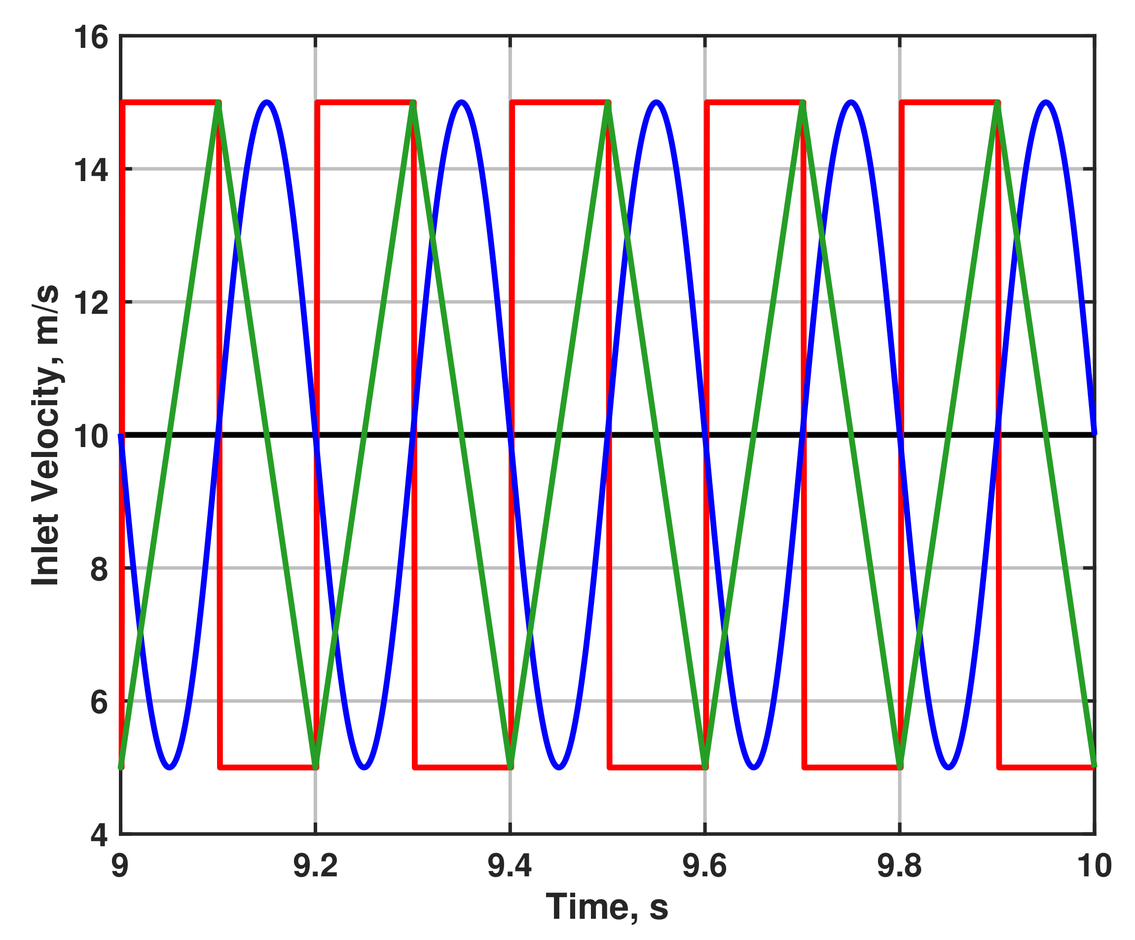
3.1. Comparison of Resulting Inlet Velocity Profiles

The different specification methods for the inlet velocity boundary condition produce slight variations in the inlet velocities applied during the simulations. In Figure 3, it is seen that the average inlet velocity is the same for all cases as in case 1, and the maximum and minimum velocities are identical for cases 2–4. Also the period of the fluctuation is the same.

3.2. Time-Averaged Quantities

We begin by analyzing the time-averaged behavior of all simulation cases. The velocity at the system inlet, the conversion at the system outlet and the uniformity index of the reactant mass fraction field half-way through the monolithic reactor are given in Table 4.

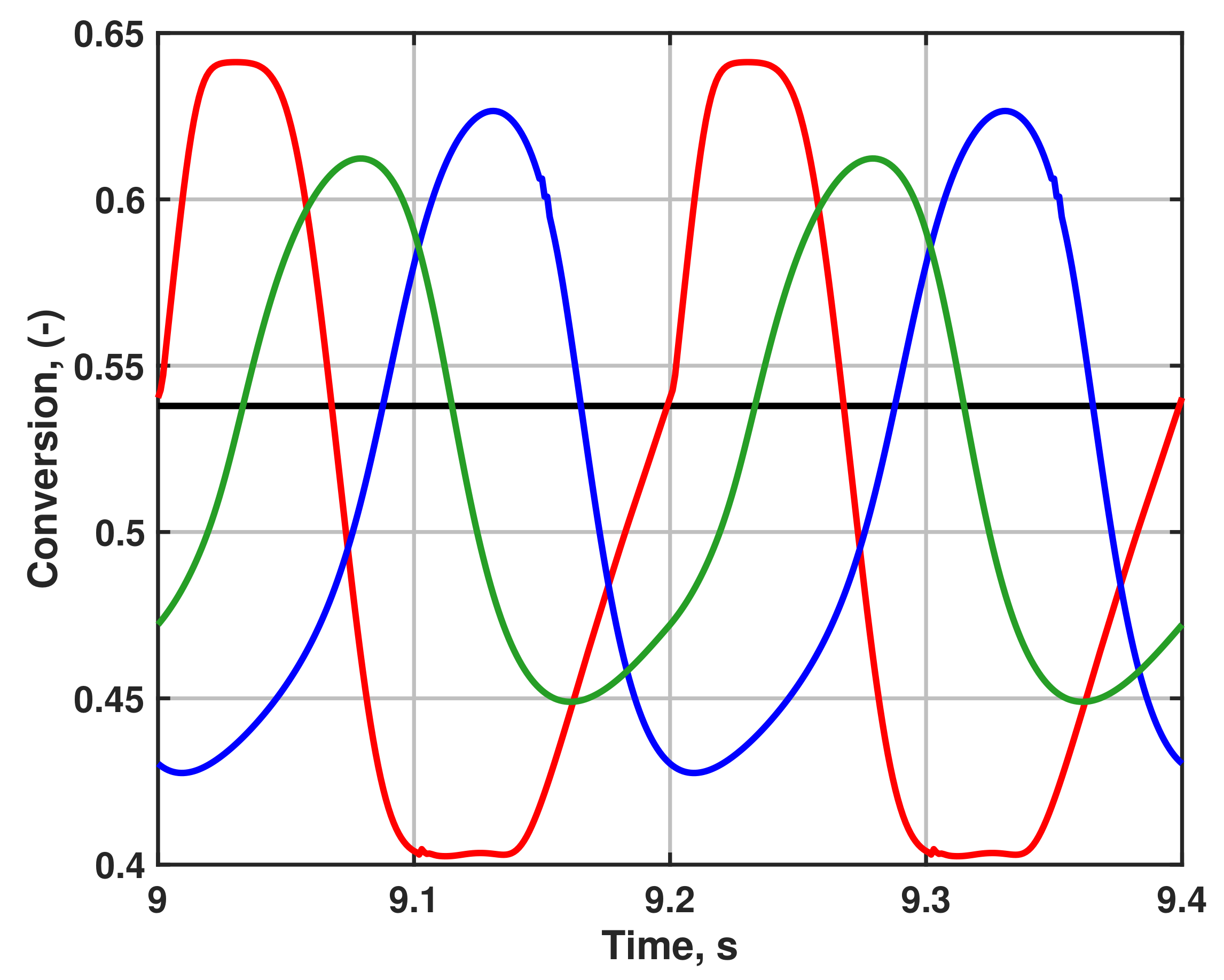
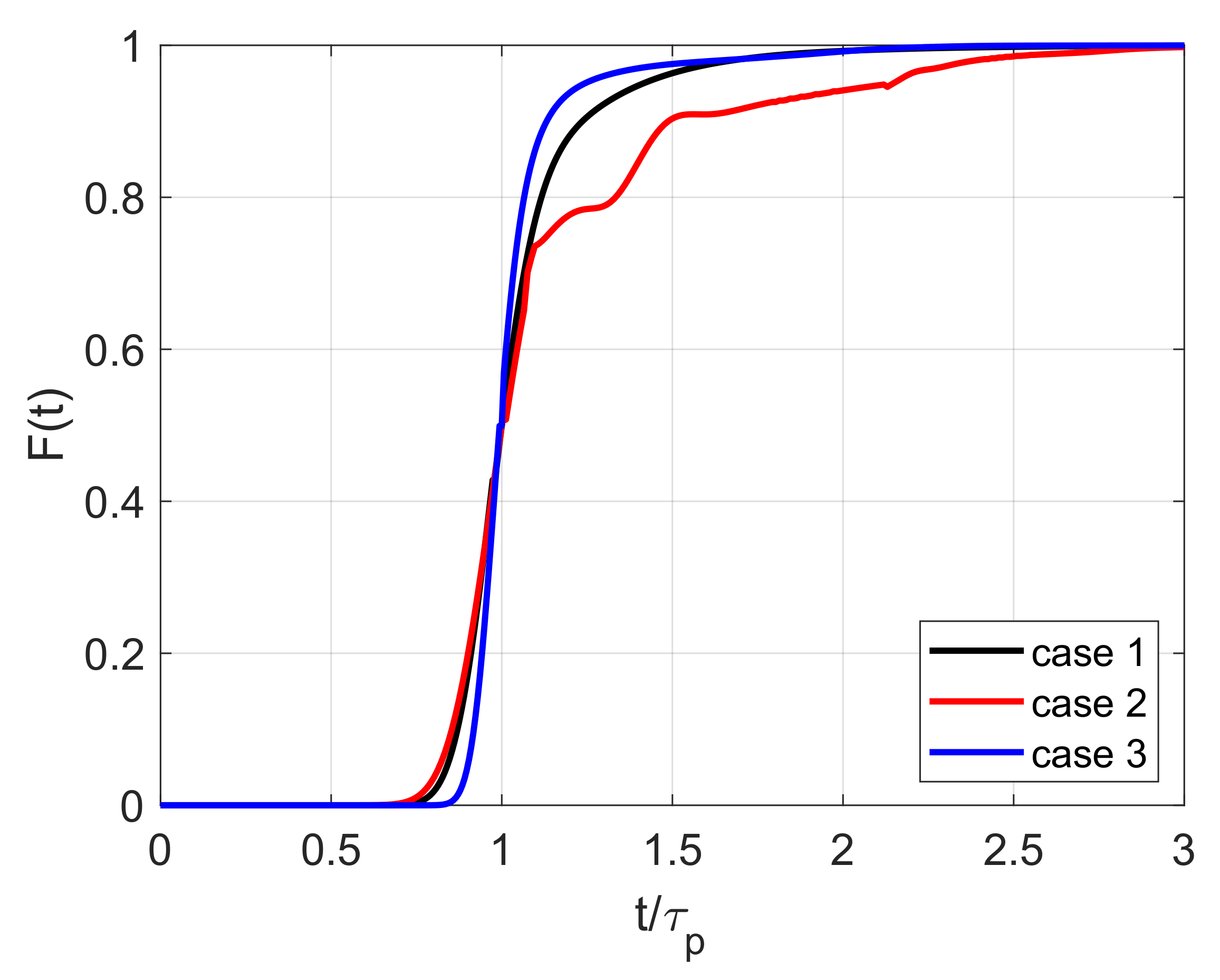
3.3. Time-Resolved Quantities

Figure 4 illustrates how the reactant conversion varies with time for systems where the inlet velocity is either constant (case 1) or varies in a step-wise (case 2), sinusoidal-like (case 3), or sawtooth-like (case 4) manner. As was seen in Table 4, the time-averaged inlet velocity was the same for all of these cases whereas the time-averaged conversions differed. It is evident from Figure 4 that the conversions vary with time in a non-trivial manner when the velocity is not constant. It is also clear that there is a temporal shift in the response in the outlet conversion to changes to the inlet velocity that depend on the flow retention time in the system, which in itself varies with time and with the velocity prescription method.
It is to be expected that the time-averaged conversion differs between cases as a reflection of that various amounts of time are spent at velocities higher and lower than the average inlet velocity, in combination with that conversion is a non-linear function of velocity. Interestingly, the observed maximum and minimum conversions do not agree between cases even though the maximum and minimum inlet velocities do. This observation can be explained by the actions of dispersion mechanisms in the monolith and the outlet cone and pipe. We may thus conclude that the influence of dispersion must also depend on the details of the variation of the inlet velocity, and that such effects affect the time-resolved concentration fields exiting the system.
A more comprehensive exposition of this phenomenon can be appreciated from observing the spatio-temporal evolution of the reactant concentration field when the inlet velocity fluctuates, as illustrated for case 2 in Figure 5. A number of observations can be made here that substantiate the previous discussion: First, it is clear that the reactant mass fraction is always decreasing in the streamwise direction inside the reactor (cf. the panel at t = 9.10 s). However, it is also apparent that the reactant mass fraction is not always monotonically decreasing in the streamwise direction throughout the entire system (as can for example be seen from the panel at t = 9.16 s, where a minimum in the reactant concentration is observed in the cone behind the reactor). Consequently, a plug of low reactant concentration (high local conversion) emerges at t 9.13 s and moves towards the outlet, reaching it sometime before t 9.22 s. Finally, we note that the conversion is lowest at t = 9.10 s and highest at t = 9.22 s in the currently observed time range. This observation is in agreement with the characterization in Figure 4 and, when taken together with the “plug formation” phenomenon just discussed, explains why the conversion signal at the system outlet goes through three stages between t = 9.10 s and t = 9.20 s. The constant low-conversion stage corresponds to the sudden velocity decrease at t = 9.10 s, which causes the current conversion level to linger at the outlet. The modest rate of increase of conversion that follows between t 9.14 s and t 9.20 s corresponds to the emergence of the high-conversion plug that forms inside the monolith after the sudden decrease of the inlet velocity. Finally, the steeper rate of conversion increase between t 9.20 s and t 9.22 s corresponds to the faster flushing out of the high-conversion fluid when the inlet velocity suddenly increases again at t = 9.20 s.
The behavior of the uniformity index, as depicted in Figure 6, exhibits quite pronounced variations with the inlet velocity prescription method. The reactant concentration field is most uniform when the inlet velocity is low, which may be confirmed by the emergence of a peak in the uniformity index for low-velocity conditions for all cases. The smoother velocity variations in cases 3 and 4 translate to more subtle variations in uniformity, whereas the step-wise pattern of case 2 (the red line in Figure 6) tends to amplify temporal fluctuations in the reactant concentration field inside the monolith.
The cumulative distribution functions (CDFs) for cases 1, 2 and 3 are compared in Figure 7. It is seen that a constant inlet velocity (case 1) produces a smooth-looking CDF that is characterized by a long tail at high values of F, indicating that some fluid spend a proportionally much longer time than the average in the system. The reason for this behavior is the presence of recirculation zones in the cones. The longer residence time of the fluid in these regions is counterbalanced by the faster path through the system along the centerline.
The sinusoidal inlet velocity variation produces a more narrow residence time distribution, as seen from the steeper gradient of the CDF for case 3 in Figure 7. At the same time, the step-like velocity variations in case 2 result in an almost wobbling characteristic of the CDF, where some fluid parcels exit even quicker than in cases 1 and 3, to be followed by pockets of slower fluid intermittently ejected after the main flow passage through the system has ended. It should be noted here that the step changes to the inlet velocity in case 2 occur almost exactly every τ (e.g., step change every 0.1 s and τ = 0.095 s). The intermittent behavior observed in F ( t ) for case 2 is thus related to internal flow phenomena and not a mere transmittance of inlet fluctuations to the outlet. In conclusion, the CDF analysis efficiently illustrates the differences in dispersion mechanisms (cf. Figure 4) that may be provoked for the same geometrical system by simply varying the temporal specification of the inlet velocity.

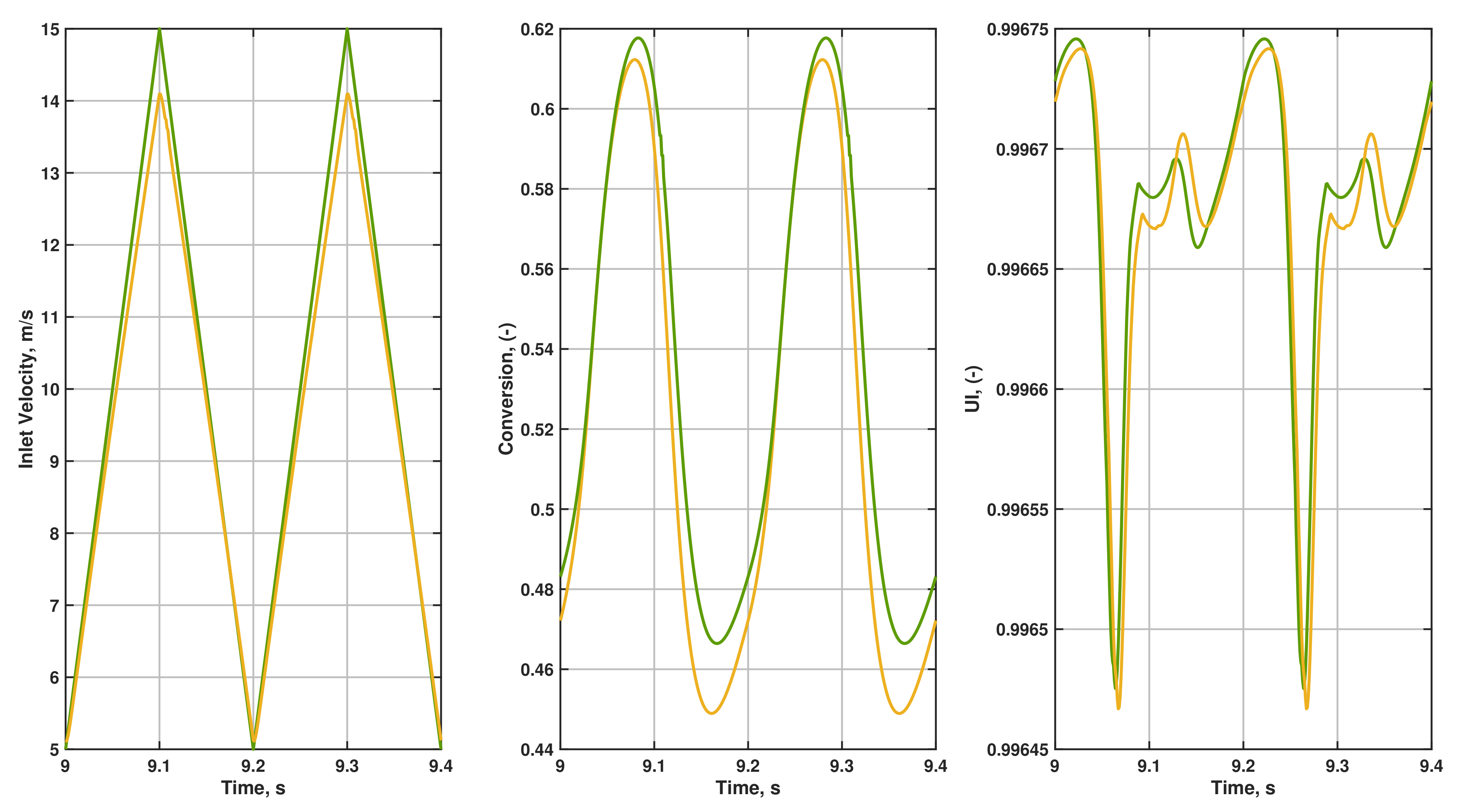
3.4. Influence of Prescribing Pressure Instead of Velocity at the Inlet Boundary

The driving pressure in cases 2B, 3B and 4B was chosen so as to produce an inlet velocity of 10 m/s at steady-state. It can be noted from Figure 8 that the inlet velocities of cases 2 and 2B match during the low-velocity periods, but not during the high-velocity periods where the pressure method results in lower maximum velocities. This effect arises due to the non-negligible influence of inertial losses at high velocity, which scale with velocity squared. Hence, a 50% decrease in the inlet pressure results in a 50% decrease of the inlet velocity, whereas a similar pressure increase cannot produce the same increase in velocity due to larger losses.
Another interesting feature of the pressure method is the intrinsic smoothness of the velocity variation upon a step change. Whereas case 2 exhibits a definitive step-like pattern in Figure 8, case 2B yields a smoother approach of the inlet velocity to the set values, both upon increases and decreases of the inlet pressure. The explanation behind this behavior is that the pressure-inlet boundary condition drives a flow towards the outlet, the velocity of which depends on the overall losses in the system, which are themselves functions of the local velocities and velocity gradients. Any step change to the inlet pressure is therefore followed by an adjustment phase where the flow field develops to accommodate the new boundary conditions. In contrast, a direct change of the velocity on the inlet boundary leaves no room for such adjustments, as the pressure field responds immediately in an incompressible flow. Figure 8 thus implies that prescribing pressures, rather than velocities, at the domain inlet will alleviate some of the artificial character introduced by boundary conditions that are discontinuous in time.
The outlet conversion and the reactant concentration distribution inside the monolith follow similar patterns for cases 2 and 2B, as shown in Figure 9. Interestingly, the highest mixed-cup conversion at the outlet attained in case 2B is lower than that for case 2, despite the fact that the lowest inlet velocity (producing the highest conversion) is identical for both cases. This observation underlines the role played by dispersion downstream of the monolith in affecting the average conversion.
Cases 3 and 3B show the differences between prescribing a sinusoidal inlet velocity or a sinusoidal inlet pressure. Similarly to case 2B, the peak pressure in case 3B is not able to drive the same peak velocity as in case 3. Apart from some minor dampening of the temporal variations in the uniformity index directly after the lowest valley, the behavior of both cases is in good agreement as shown in Figure 10.
A comparison of cases 4 and 4B, where a saw-tooth profile is prescribed for the inlet velocity or pressure, yields a similar picture (cf. Figure 11). Again, it is the half of the repeating period (e.g., from t 9.075 s to t 9.175 s in the right-hand panel of Figure 11) directly after the lowest valley that exhibits the most pronounced dependence on the subtle differences in the effective velocity through the system.

3.5. Influence of Inlet Temperature Variations

Figure 12 illustrates the outlet conversion and monolith uniformity index variations when the inlet velocity is fixed and the inlet temperature fluctuates in a sinusoidal-like pattern. Two observations stand out: conversion does not fluctuate much, and there appears to be a slow drift towards lower values even after t = 9 s.
The first observation is explained by the that the gas-phase density is obtained from the ideal gas law. Consequently, the mass-flow rate at the inlet varies with time with this case specification even though the inlet velocity is constant. Moreover, the mass-flow variations are inversely proportional to the density variations, which in turn are inversely proportional to temperature. The mass-flow into the system therefore fluctuates proportionally to the temperature on the inlet. With an increase in the system throughput, the retention time decreases, and thus the system has a built-in mechanism to counteract increases in conversion at higher temperature by shorter retention times (and vice versa at lower temperatures). The end-result is that the observed fluctuations are mild.
The second observation in Figure 12 that there is a long-term drift of the outlet conversion towards lower values even after the initial flow transients are long gone is explained by the longer time scale for thermal response of an aftertreatment system (cf. Table 1). The equilibration of the monolith brick to the long-term thermal quasi-steady-state conditions takes longer than 10 s and the process is thus still not completed when the signals in Figure 12 are extracted.

4. Discussion

Fluctuations and pulsations in the boundary conditions to automotive aftertreatment systems are naturally occurring and influence flow, heat and mass transfer, as well as local reaction conditions. All these influences translate to a complex coupling between boundary conditions and the macroscopic system behavior and performance. In CFD simulations of the reactive flow in aftertreatment systems, details in the boundary condition specification therefore become important, but have not yet received much attention in the scientific literature. These details include both aspects of the physics reflected (or neglected) by the prescribed boundary conditions, as well as technical considerations with regard to what variables to prescribe at the boundaries and the effects of such choices on simulation robustness and accuracy.
The analyses presented in the present work illustrate that the inferences that can be made from steady-state simulations at fixed operational points are limited, as there are no relevant driving conditions representative of such operation and the results are not the same as for simulations resolving all or some of the upstream fluctuations. The introduction of time-varying boundary conditions that correctly reflect upstream flow property fluctuations should therefore be favored over routine steady-state CFD. This conclusion is further supported by the fact that complex pipe shapes with bends and curvatures have the potential to generate strong and unsteady secondary flows in hot exhaust flows [17], which necessitate unsteady simulation to correctly assess the interaction with pulsations [18].
However, the incompressibility assumption adopted in the present work also imposes a limitation on the type of pulsations that can be resolved. More specifically, this assumption implies that pulsations are driven by mass flow rather than by pressure waves. The incompressible flow treatment is traditionally considered acceptable for the conventional placement of the aftertreatment system devices downstream of the turbocharger [19]. Furthermore, the range of pressure pulsations has been shown to decrease sharply along the flow path through a muffler due to the pressure drops associated with sudden reductions and expansions [20]. Even so, we stress that neglecting sound waves does impose an upper bound on the region of validity of the inlet pulsation flow frequencies that may be studied.
The idealized inlet velocity boundary conditions investigated in the current work should be interpreted as models for different types of temporal variations observed in real-world conditions. In this perspective, the sinusoidal variation represents well-resolved boundary information, whereas the saw-tooth signal represents interpolation in sparsely sampled boundary information, and the square wave mimics interpolation in sampled information at coarser temporal resolution. Whereas the square wave is discontinuous in time theoretically, it will here be felt as a sharp increase from one time step to another, essentially replicating the behaviour of the saw-tooth signal over a much shorter duration. Real-world boundary information could be expected to contain a mixture of these characteristics depending on the evolution of the mean and the fluctuations in the signal, the experimental sampling interval used and the computational time step employed.
In the present work, the chemical kinetics have been described by a first-order heterogeneous reaction. In future works, extension to a full micro-kinetic model could be investigated. A more comprehensive description of the sorption processes, parallel reactions, and heat-of-reaction effects—although outside the scope of the current investigation—could be expected to reveal how fluctuations in local flow and heat and mass transfer conditions may trigger and interact with such more complex fluctuations in the chemical kinetics.
The application of the conventional porous medium description of the monolith brick in its current implementation neglects the possible influence of decaying turbulence in the entrance region of the monolith channels. Such turbulent inlet effects have previously been shown to interact with the chemical kinetics and cannot be ruled out as a moderator of fluctuations that are indirectly controlled by boundary condition variations [21,22,23]. Previous investigations indicate that significant effects on heat and mass transfer may be expected if periodic disruptions of the boundary layers can be realized through flow oscillations [24]. Moreover, the porous nature of the walls of the monolithic reactor should be expected to increase the local turbulence levels in the near-wall region [25,26], which may also increase the net transfer efficiencies [27].

5. Conclusions

The following conclusions can be made from the present work:
  • Fluctuations and pulsations in the incoming flow to a monolithic reactor in an aftertreatment system both affects the transient response of the reactor as well as its time-averaged performance;
  • Pulsations act via two main mechanisms: modulation of the average retention time in the catalyst and modulation of the retention time distribution via the flow maldistribution over the reactor cross-section;
  • The range spanned by the mixed-cup conversion at the outlet of an aftertreatment system is not identical for geometrically identical systems spanning the same velocity range, as dispersion mechanisms inside the monolith and the outlet cone and pipe sections create mixing environments that depend on the fluctuations and their interactions with the geometry itself:
  • The dispersion mechanisms depend in a non-trivial way on the temporal specification of the flow inlet boundary condition;
  • Simulations of phenomena that depend on time-resolved boundary conditions from experiments are likely to require interpolation in sparsely sampled information—the method of recreating the signal at the boundary may then influence the results;
  • Prescribing an inlet pressure rather than an inlet velocity in simulations of monolithic reactors in aftertreatment systems results in smoother transient boundary condition profiles and avoidance of intermittent flow discontinuity propagation through the system, at the expense of a loss of direct proportionality between fluctuation and resulting velocity (due to non-linear losses at high velocities);
  • Temperature fluctuations have a potential to affect reaction rates profoundly due to the strong non-linear dependence, but the effect is partially out-weighted by anti-correlated retention-time fluctuations.
The inferences and analysis presented in this work is of benefit for researchers and engineers working with exhaust gas aftertreatment systems and monolithic reactors in general, and researchers and engineers dealing with advanced reactive computational fluid dynamics-simulations of such systems in particular.

Author Contributions

Conceptualization, P.C.N., H.S. and J.S.; Data curation, P.C.N.; Formal analysis, P.C.N.; Funding acquisition, J.S.; Investigation, P.C.N. and H.S.; Methodology, P.C.N. and H.S.; Project administration, J.S.; Resources, H.S. and J.S.; Software, P.C.N. and H.S.; Supervision, H.S. and J.S.; Validation, P.C.N.; Visualization, P.C.N.; Writing—original draft, P.C.N.; Writing—review & editing, H.S. and J.S. All authors have read and agreed to the published version of the manuscript.

Funding

Financial support from the Combustion Engine Research Centre (CERC) is gratefully acknowledged.

Data Availability Statement

The data reported in the present manuscript can be provided by the authors upon request.

Conflicts of Interest

The authors declare no conflict of interest. The funders had no role in the design of the study; in the collection, analyses, or interpretation of data; in the writing of the manuscript, or in the decision to publish the results.

Abbreviations

The following abbreviations are used in this manuscript:
CDFCumulative Distribution Function
CFDComputational Fluid Dynamics
MUSCLMonotonic Upstream-centered Scheme for Conservation Laws
RHSRight Hand Side
SCMSingle Channel Model
SSTShear Stress Transport
URANSUnsteady Reynolds-Averaged Navier-Stokes

References

  1. Heck, R.M.; Farrauto, R.J.; Gulati, S.T. Catalytic Air Pollution Control: Commercial Technology; John Wiley & Sons: Hoboken, NJ, USA, 2016. [Google Scholar]
  2. Deutschmann, O. Modeling of the interactions between catalytic surfaces and gas-phase. Catal. Lett. 2015, 145, 272–289. [Google Scholar] [CrossRef]
  3. Martin, A.P.; Will, N.S.; Bordet, A.; Cornet, P.; Gondoin, C.; Mouton, X. Effect of flow distribution on emissions performance of catalytic converters. SAE Trans. 1998, 107, 384–390. [Google Scholar]
  4. Chen, J.; Yang, H.; Wang, N.; Ring, Z.; Dabros, T. Mathematical modeling of monolith catalysts and reactors for gas phase reactions. Appl. Catal. Gen. 2008, 345, 1–11. [Google Scholar] [CrossRef]
  5. Walander, M.; Sjöblom, J.; Creaser, D.; Agri, B.; Löfgren, N.; Tamm, S.; Edvardsson, J. Modelling of mass transfer resistances in non-uniformly washcoated monolith reactors. Emiss. Control. Sci. Technol. 2021, 7, 153–162. [Google Scholar] [CrossRef]
  6. Chakravarthy, V.K.; Conklin, J.C.; Daw, C.S.; D’Azevedo, E.F. Multi-dimensional simulations of cold-start transients in a catalytic converter under steady inflow conditions. Appl. Catal. A Gen. 2003, 241, 289–306. [Google Scholar] [CrossRef]
  7. Bella, G.; Rocco, V.; Maggiore, M. A Study of Inlet Flow Distortion Effects on Automotive Catalytic Converters. J. Eng. Gas Turbines Power 1991, 113, 419–426. [Google Scholar] [CrossRef]
  8. Zygourakis, K. Transient operation of monolith catalytic converters: A two-dimensional reactor model and the effects of radially nonuniform flow distributions. Chem. Eng. Sci. 1989, 44, 2075–2086. [Google Scholar] [CrossRef]
  9. Bressler, H.; Rammoser, D.; Neumaier, H.; Terres, F. Experimental and predictive investigation of a close coupled catalyst converter with pulsating flow. SAE Trans. 1996, 105, 255–267. [Google Scholar]
  10. Liu, Z.; Benjamin, S.F.; Roberts, C.A. Pulsating flow maldistribution within an axisymmetric catalytic converter-flow rig experiment and transient cfd simulation. SAE Tech. Pap. 2003. [Google Scholar] [CrossRef]
  11. Benjamin, S.; Roberts, C.; Wollin, J. A study of pulsating flow in automotive catalyst systems. Exp. Fluids 2002, 33, 629–639. [Google Scholar] [CrossRef]
  12. Jeong, S.-J. A full transient three-dimensional study on the effect of pulsating exhaust flow under real running condition on the thermal and chemical behavior of closed-coupled catalyst. Chem. Eng. Sci. 2014, 117, 18–30. [Google Scholar] [CrossRef]
  13. Tsinoglou, D.; Koltsakis, G. Influence of pulsating flow on close-coupled catalyst performance. J. Eng. Gas Turbines Power 2005, 127, 676–682. [Google Scholar] [CrossRef]
  14. Ström, H.; Sasic, S.; Andersson, B. Turbulent operation of diesel oxidation catalysts for improved removal of particulate matter. Chem. Eng. Sci. 2012, 69, 231–239. [Google Scholar] [CrossRef]
  15. Fogler, H.S. Elements of Chemical Reaction Engineering; Pearson Education: London, UK, 1999. [Google Scholar]
  16. Menter, F.R. Two-equation eddy-viscosity turbulence models for engineering applications. AIAA J. 1994, 32, 1598–1605. [Google Scholar] [CrossRef] [Green Version]
  17. Bodin, O.; Wang, Y.; Mihaescu, M.; Fuchs, L. LES of the Exhaust Flow in a Heavy-Duty Engine. Oil Gas Sci. Technol. Rev. IFP Energies Nouv. 2014, 69, 177–188. [Google Scholar] [CrossRef] [Green Version]
  18. Semlitsch, B.; Wang, Y.; Mihaescu, M. Flow effects due to pulsation in an internal combustion engine exhaust port. Energy Convers. Manag. 2001, 86, 520–536. [Google Scholar] [CrossRef] [Green Version]
  19. Torregrosa, A.J.; Serrano, J.R.; Arnau, F.J.; Piqueras, P. A fluid dynamic model for unsteady compressible flow in wall-flow diesel particulate filters. Energy 2011, 36, 671–684. [Google Scholar] [CrossRef] [Green Version]
  20. Kim, M.-H. Three-Dimensional Numerical Study on the Pulsating Flow Inside Automotive Muffler with Complicated Flow Path. SAE Trans. 2001, 110, 805–811. [Google Scholar]
  21. Ström, H.; Sasic, S. Heat and mass transfer in automotive catalysts—The influence of turbulent velocity fluctuations. Chem. Eng. Sci. 2012, 83, 128–137. [Google Scholar] [CrossRef]
  22. Tanno, K.; Kurose, R.; Michioka, T.; Makino, H.; Komori, S. Direct numerical simulation of flow and surface reaction in de-NOx catalyst. Adv. Powder Technol. 2013, 24, 879–885. [Google Scholar] [CrossRef]
  23. Cornejo, I.; Nikrityuk, P.; Hayes, R.E. Turbulence Decay Inside the Channels of an Automotive Catalytic Converter Monolith. Emiss. Control Sci. Technol. 2017, 3, 302–309. [Google Scholar] [CrossRef]
  24. Hewakandamby, B.N. A numerical study of heat transfer performance of oscillatory impinging jets. Int. J. Heat Mass Transf. 2009, 52, 396–406. [Google Scholar] [CrossRef]
  25. Suga, K.; Matsumura, Y.; Ashitaka, Y.; Tominaga, S.; Kaneda, M. Effects of wall permeability on turbulence. Int. J. Heat Fluid Flow 2010, 31, 974–984. [Google Scholar] [CrossRef]
  26. Suga, K. Understanding and Modelling Turbulence Over and Inside Porous Media. Flow Turbul. Combust. 2016, 96, 717–756. [Google Scholar] [CrossRef]
  27. Andersson, R.; Andersson, B. Enhanced mass and heat transfer in catalytic reactors. Catal. Today 2013, 216, 117–120. [Google Scholar] [CrossRef]
Figure 1. Overview of the computational geometry used in the present work. The flow goes from left to right. The domain is 2D axisymmetric and the horizontal line from the middle of the inlet represents the axis of symmetry. The dark yellow section is the monolith brick.
Catalysts 12 00613 g001
Figure 2. Inlet velocities and temperatures over time as obtained in cases 1, 2, 3 and 4. The blue lines and the red lines represent velocity and temperature respectively.
Catalysts 12 00613 g002
Figure 3. Inlet velocities over time as obtained in cases 1 (black), 2 (red), 3 (blue) and 4 (green).
Catalysts 12 00613 g003
Figure 4. Conversion of reactant at system outlet over time as obtained in cases 1 (black), 2 (red), 3 (blue) and 4 (green).
Catalysts 12 00613 g004
Figure 5. Five snapshots of the reactant mass fraction fields for case 2 (at t = 9.10 s, t = 9.13 s, t = 9.16 s, t = 9.19 s, and t = 9.22 s). The inlet velocity decreases from 10 m/s to 5 m/s at t = 9.10 s and increases to 10 m/s again at t = 9.20 s. The existence of a low-mass-fraction region emerging from the end of the monolithic reactor is clearly visible at times t = 9.13–9.19 s, indicating that the reactant mass fraction is not monotonically decreasing along the streamwise direction when the inlet velocity is fluctuating.
Catalysts 12 00613 g005
Figure 6. Uniformity index of reactant field half-way through the monolith brick over time as obtained in cases 1 (black), 2 (red), 3 (blue) and 4 (green).
Catalysts 12 00613 g006
Figure 7. Cumulative distribution function F ( t ) for a step change in concentration of a non-reacting species at the system inlet (i.e., cases 1, 2 and 3 with R = 0 in Equation (12)).
Catalysts 12 00613 g007
Figure 8. Resulting inlet velocity profiles over time as obtained in cases 2 (red) and 2B (brown).
Catalysts 12 00613 g008
Figure 9. Resulting conversion at the system outlet (left) and uniformity index of the reactant field (right) over time as obtained in cases 2 (red) and 2B (brown).
Catalysts 12 00613 g009
Figure 10. Resulting inlet velocity profiles (left), conversion at the system outlet (middle) and uniformity index of the reactant field (right) over time as obtained in cases 3 (blue) and 3B (purple).
Catalysts 12 00613 g010
Figure 11. Resulting inlet velocity profiles (left), conversion at the system outlet (middle) and uniformity index of the reactant field (right) over time as obtained in cases 4 (green) and 4B (orange).
Catalysts 12 00613 g011
Figure 12. Resulting conversion at the system outlet (left) and uniformity index of the reactant field (right) over time as obtained in case 1C, where the inlet velocity is constant but temperature is fluctuating.
Catalysts 12 00613 g012
Table 1. Timescales in automotive catalysis.
PhenomenonTimescale
Turbo pulsations O ( ms )
Lambda control O ( s )
Driver interaction O ( s )
Catalyst heatup O ( min )
Table 2. Material properties.
PropertyValue
ρ ideal gas law 1
μ Sutherland’s law 2
c p 1006.43 J/(kg·K)
k 0.0454 W/(m·K)
D A B 2.88 × 10 5 m2/s
1   M w = 28.966 kg/kmol. 2   µ 0 = 1.716 × 10 5 kg/(m·s), T 0 = 273.11 K, S = 110.56 K.
Table 3. The boundary condition specifications of the cases investigated in the present work. The flow inlet boundary condition is either a specified velocity or a specified pressure. The inlet temperature boundary condition is a specified temperature.
CaseFlow Inlet Boundary Condition 1Temperature Boundary Condition 2
Case 1 U ( t ) = U 0 T ( t ) = T 0
Case 1C U ( t ) = U 0 T ( t ) = T 0 + Δ T sin 2 π t / Δ t
Case 2 U ( t ) = U 0 + Δ U if mod ( rem ( t , Δ t ) ) = 0 U 0 Δ U else T ( t ) = T 0
Case 2B P ( t ) = P 0 + Δ P if mod ( rem ( t , Δ t ) ) = 0 P 0 Δ P else T ( t ) = T 0
Case 3 U ( t ) = U 0 + Δ U sin π t / Δ t T ( t ) = T 0
Case 3B P ( t ) = P 0 + Δ P sin π t / Δ t T ( t ) = T 0
Case 4 U ( t ) = Δ U + U 0 t / Δ t if mod ( rem ( t , Δ t ) ) = 0 3 Δ U U 0 t / Δ t else T ( t ) = T 0
Case 4B P ( t ) = Δ P + P 0 t / Δ t if mod ( rem ( t , Δ t ) ) = 0 3 Δ P U 0 t / Δ t else T ( t ) = T 0
1   U 0 = 10 m/s, Δ U = U 0 / 2 , P 0 = 1004.3067 Pa, Δ P = P 0 / 2 and Δ t = 0.1 s. 2   T 0 = 573 K, Δ T = 50 K and Δ t = 0.1 s.
Table 4. Time-averaged results for inlet velocity, conversion at system outlet and uniformity index inside the monolith brick. The variation intervals reported are the standard deviations. Averages and standard deviations are recorded for the last second of a 10-second run.
CaseVelocity [m/s]ConversionUniformity IndexTemperature [K]
Case 1 10.0 0.538 0.9967 573.0
Case 1C 10.0 ± 0.00 0.498 ± 0.001 0.9971 ± 1.64 × 10 4 573.0 ± 35.36
Case 2 10.0 ± 5.00 0.503 ± 0.090 0.9966 ± 2.79 × 10 4 573.0
Case 2B 9.60 ± 4.52 0.519 ± 0.085 0.9966 ± 2.45 × 10 4 573.0
Case 3 10.0 ± 3.54 0.514 ± 0.073 0.9967 ± 8.71 × 10 5 573.0
Case 3B 9.66 ± 3.25 0.528 ± 0.069 0.9967 ± 8.83 × 10 5 573.0
Case 4 10.0 ± 2.89 0.522 ± 0.060 0.9967 ± 6.19 × 10 5 573.0
Case 4B 9.68 ± 2.66 0.535 ± 0.056 0.9967 ± 6.41 × 10 5 573.0
Publisher’s Note: MDPI stays neutral with regard to jurisdictional claims in published maps and institutional affiliations.

