1. Introduction
How production is organized within and across firms crucially affects the welfare of the final consumers and is, naturally, the core concern of industrial organization and related fields. One of the factors that shape the key market outcomes is the intensity of competition and the variety of available products. In this regard, different instances of exclusionary practices in vertically related industries, between upstream and downstream firms, have drawn the attention of regulators and anti-trust authorities and have been the focus of influential academic research, with the foreclosure of some producers viewed with suspicion in most of the cases. Yet, there are also other factors that play a crucial role in determining market outcomes and welfare, including efficiency in production. While exclusionary practices have been extensively studied in the literature, less attention has been given to the role and nature of exclusivity in dynamic environments.
In this paper, we introduce dynamic interactions in a vertical chain through learning-by-doing in production. This is performed in a simple way: there is an upstream duopoly, where the production of each firm may become more efficient according to the accumulation of production over time. The upstream firms produce either complements or substitutes, with horizontal product differentiation taking the form of “love for variety”. A downstream monopolist can receive the products of the upstream firms and has the power to set linear wholesale contract terms. Crucially, the game lasts for two periods. In each period, the retailer sets the contract terms to each of the upstream firms, which can either accept or reject their contract offers. Following that stage, the retailer sells the products to the final consumers and pays the upstream firms according to the contracts that have been agreed. When the game proceeds to the second period, the costs of the upstream firms may have been reduced based on their first period production level.
In this setting, we explore the tensions between assuring access to competing varieties and lowering production costs via learning-by-doing. Exclusion arises implicitly when the dominant retailer offers very disadvantaged contract terms to an upstream firm, and, thus, forces it to stay out of the market. Thus, exclusivity does not arise by a dominant upstream firm’s denial to supply some downstream firms with the essential input that it produces.
1 Instead, the retailer is a large player, and the upstream firms can reach the final consumers only via this retailer. Our analysis can be applicable to a multiproduct firm where production is characterized by the learning hypothesis or to a strategic buyer that can manipulate the learning process through their product choice. The role of the intermediary is studied by examining whether the existence of this firm intensifies the learning process compared to the case where there is no intermediary in the market, but the upstream firms compete directly in the final market.
Within such a framework, interesting questions arise: How does the final market outcome depend on the intensity of learning-by-doing and product differentiation? Does the retailer choose to carry only one product to intensify the learning process? Under what conditions do exclusivity and, thus, customer foreclosure emerge? Under what conditions may they be beneficial for the final consumers and the firms? Does the market competition favor an outcome with lower prices or with more variety in the market? Is the presence of the retailer in the market necessary to intensify the learning process?
The food industry is a leading motivating example, corresponding to such vertical structure models and one that has been attracting the attention of policy makers and even the popular press. In the last couple of decades, large supermarkets have emerged and become powerful in their transactions with upstream suppliers in many industries. Other examples include large tour operators trading with airlines and hotels or general retailers such as Wal-Mart. The issue of exclusionary practices is also central in manufacturing, like in the automobile sector (see, e.g., Brenkers and Verboven, 2005) [
1].
The fact that learning-by-doing can be an important factor in production processes has been documented in a number of business units and sectors, such as the agriculture industry where sustainable farming relies on learning from the experience gained over multiple growing seasons. Furthermore, this is the case in manufacturing contexts, such as in the automobile industry where Toyota Production System is based on the concept of “Kaizen”, i.e., continuous improvement, through learning from experience. Other leading examples of learning-by-doing in production include the construction industry and the software development industry.
In the static version of our model, the retailer always chooses to carry both products. In a one-period setting, there is no learning and exclusivity reduces the variety in the market without reducing the production costs or the prices. In the dynamic model, exclusivity arises in equilibrium when products are close substitutes. In contrast, when products are complements or not close substitutes, both are purchased in both periods. This result follows from two opposite effects. There is a trade-off between lower costs due to learning and more product varieties in the market. When product differentiation is low, the “learning” effect dominates the “product variety” effect, and the total profits of the chain and the consumer’s surplus are higher when one product is excluded from the market. It follows that exclusivity is welfare-enhancing. Furthermore, relative to the non-exclusivity case, the product prices in both periods are lower when exclusivity is imposed by the retailer. However, the rate of learning is not equal to the social optimum and the social planner would impose exclusivity more often compared to the retailer. We also maintain that the presence of the downstream intermediary is necessary in intensifying the learning-by-doing process when products are complements or when products are close substitutes, and the retailer imposes exclusivity.
Our paper contributes to two different fields in the literature within industrial organization: vertical contracting and learning-by-doing and business organization. Each of these contains very important papers and it is too vast to survey here. We only refer to work that is more closely related to our analysis. First, numerous contributions highlight the impact of vertical contracting and, in particular, the impact of exclusionary behavior on market competition. For a review and some key results on vertical foreclosure, see Rey and Tirole (2007) [
2]. Krattenmaker and Salop (1986) [
3] argue that contracts with input suppliers can be fertile ground for raising competitor’s cost and Aghion and Bolton (1987) [
4] demonstrate that contracts between buyers and sellers will be signed for entry-prevention purposes. Mathewson and Winter (1987) [
5], Besanko and Perry (1993) [
6], and O’Brien and Shaffer (1993) [
7] derive that exclusive arrangements can have desirable welfare properties.
2 The opportunistic behavior is faced through exclusivity according to McAfee and Schwartz (1994) [
8]. We obtain that exclusivity is welfare-improving, compared to non-exclusivity, due to learning in the production.
Rey and Stiglitz (1995) [
9] obtain maintain that, when goods are close substitutes, producers’ profits are higher under exclusive territories. We maintain that when goods are close substitutes, retailer’s profits are higher under exclusivity since the learning effect dominates the product variety effect. Foreclosure has also recently been studied in vertical contracting frameworks with vertically integrated firms by Reisinger and Tarantino (2015) [
10] and Kourandi and Pinopoulos (2023) [
11]. We depart from vertical integration and study how learning affects future production efficiency and, thus, the market exclusion of upstream producers. A dynamic setting with intertemporal linkages and input foreclosure is studied by Fumagalli and Motta (2020) [
12] and Sandiumenge i Boy (2023) [
13]. We focus on customer foreclosure.
Furthermore, there is a well-known field in the literature on common agencies that deal with exclusivity. See, for example, Martimort (1996) [
14], Bernheim and Whinston (1998) [
15], and Segal and Whinston (2000) [
16]. Further, Marx and Shaffer (2007) [
17] adopt upfront payments with bargaining power in the downstream level and find that exclusivity arises in equilibrium. In our setup, when products are close substitutes, the bottleneck retailer coordinates the purchases of the two products and takes advantage of the learning process in a more efficient way compared to the case where upstream producers directly sell their products to the final consumers. Nevertheless, relatively few papers have examined vertical chain interactions in a dynamic framework. An exemption is Chen (2005) [
18], who studies vertical disintegration in a dynamic model with learning-by-doing and downstream competition.
3 In our dynamic model with learning-by-doing, we focus, instead, on product differentiation and customer foreclosure.
The second related field in the literature examines strategic purchases in one-tier industries in a dynamic setting under the learning-by-doing hypothesis. Spence (1981) [
21] obtains the dynamic output path of a single- and then a multi-firm model and studies the open and closed loop equilibria. Fudenberg and Tirole (1983) [
22] derive the precommitment and perfect equilibria with linear demand and learning functions. A price-setting differentiated duopoly with an infinite sequence of heterogeneous buyers and uncertain demands is analyzed by Cabral and Riordan (1994) [
23], where they find the Markov perfect equilibrium and study the concept of market dominance. In an enriched version of the Cabral and Riordan model, Besanko, Doraszelski, and Kryukov (2019) [
24] use computational methods to analyze the Markov Perfect equilibrium behavior. Lewis and Yildirim (2002a) [
25] study the trade-off between experience and competition in an industry with privately cost functions and a single buyer. Meanwhile, Lewis and Yildirim (2002b) [
26] investigate how incentive regulation should be designed to encourage suppliers to develop and adopt cost-saving technologies. Recently, Sweeting et al. (2022) [
27] studied dynamic price competition when sellers benefit from learning-by-doing and buyers are long-lived and strategic, while capturing, with a single parameter, the extent to which each buyer internalizes future buyer surplus. They find that even moderate degrees of forward-looking buyer behavior may eliminate the multiplicity of equilibria and that equilibria with competition are more likely to survive.
In these models, learning-by-doing can be understood either as cost-reducing innovations or as the result of economies of scale across multiple market segments, where the different time periods play the role of different market segments. Our setup adds an extra tier in the vertical supply chain. Products are reached by the consumers via a retailer that may decide to reduce product availability. We explore the conditions under which the learning effect dominates the product variety effect in a vertical chain and find, consistently with the learning-by-doing literature, that equilibria with either more (non-exclusivity, i.e., competing suppliers) or less (exclusivity, i.e., monopoly supplier) variety can emerge depending on the level of product differentiation. Yet, our model is kept simple, especially in the sense that the power to set wholesale prices is given to the retailer. Thus, while the analysis captures the main tension between product variety and dynamic cost reduction, the richer model is necessary to address more complex issues that would arise if bargaining power was more evenly distributed across upstream and downstream firms.
The remainder of the paper is presented as follows.
Section 2 characterizes the equilibrium when the game lasts only one period. The dynamic model is analyzed in
Section 3. Consumer’s surplus and total welfare are calculated in
Section 4. In
Section 5, we derive the social planning solution and compare it to the equilibrium.
Section 6 studies the role of the intermediary in the learning process and
Section 7 concludes.
2. The Static Model
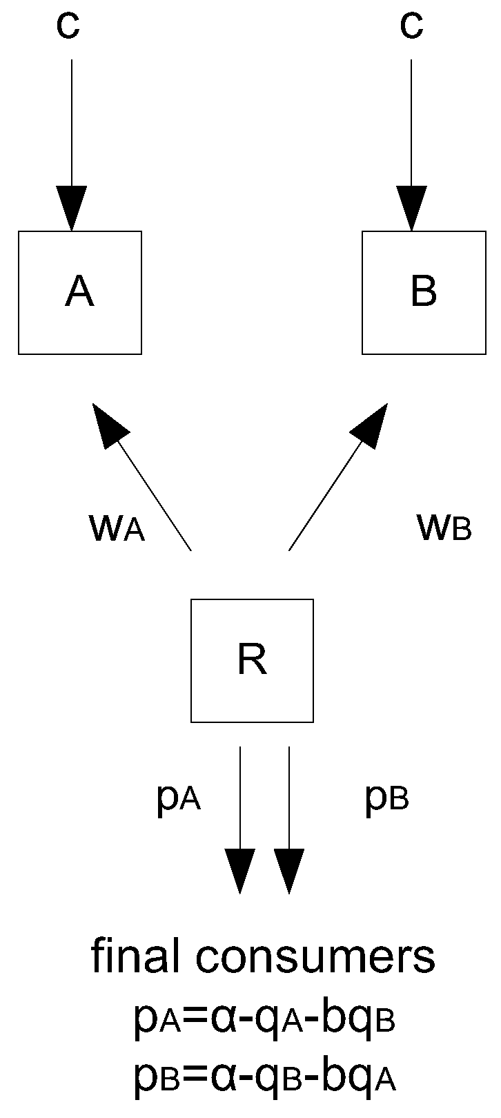
We begin our analysis by studying the potential for exclusivity to arise in a simple setting where firms compete for a single period. We consider two manufacturers, A and B, who each produce a single product with these products to be either substitutes or complements. Product differentiation is horizontal and takes the form of “love for variety”. Manufacturers supply the downstream market and have the same constant marginal production cost, c, since we focus on the possibility of exclusivity to emerge as a result of strategic interaction and not due to cost asymmetries in the upstream industry.
The downstream market is monopolized by a retailer, R, that has the power to set the contract terms which take the form of linear wholesale prices.
4 One unit of the manufacturers’ product becomes one unit of final good at zero marginal cost. The inverse final demand functions take the linear form
, where
is the retail price and
is the quantity of product
i,
,
and
is the product differentiation parameter.
5 When
b equals zero, the two products are independent. As
b approaches the unity (
) the two goods become closer substitutes and as
approaches minus one (
) the two goods become closer complements. When
b is equal to one, the goods are homogeneous and when
b is equal to minus one, the two goods are perfect complements. There is no uncertainty and all contracts are observable. The static framework is presented in
Figure 1.
We consider a three-stage game. First, the retailer sets the contract terms. Then, the manufacturers either accept or reject the contract offers and finally the retailer sells the products to the final consumers and pays the manufacturers according to their contracts. The game is solved backwards, using subgame perfection as the equilibrium concept.
In the first stage of the game, the retailer can set very disadvantaged terms to one of the two suppliers (say B) to force this supplier to reject this offer and stay out of the market. The retailer implicitly denies access of the final consumers to that firm’s product by offering a wholesale price lower than the production cost of that manufacturer.
6 First, we consider the case where both products are carried by the retailer (non-exclusivity) and then we study the corner case where the retailer chooses to carry only one product (exclusivity).
Non-exclusivity: Solving backwards, in the final stage of the game, the retailer maximizes its profits, , in the final goods market. The optimal quantities are derived by the first-order conditions.
Then, the retailer sets the wholesale prices
,
, given the individual rational constraints of the manufacturers. The manufacturers accept the offer if they obtain non-negative profits, since at the downstream level there is no alternative retailer, which leads to zero outside option for the manufacturers. Thus, the downstream monopolist sets the wholesale prices equal to the minimum possible level, that is,
for both manufacturers.
7Lemma 1. In the static model with both products carried by the retailer, we obtain: The final prices are equal to the monopoly prices. The chain profits are maximized and captured by the retailer.
Exclusivity: Assume now that, in the first stage of the game, the retailer chooses to distribute only one product, say A. Now, it maximizes its profits, , and obtains the optimal quantity by the first-order condition.
The retailer then determines the wholesale prices for the manufacturer A to accept the offer and for B to reject the offer. The retailer charges a wholesale price equal to the unit production cost to manufacturer A, , and a wholesale price lower than the production cost to manufacturer B, , to exclude this product from the market. The monopoly results are reached with the retailer to extract the vertical chain’s profits.
Lemma 2. In the static model, with one product in the market, we obtain: When products are perfect substitutes (), the results from the two subgames coincide, apart from the fact that the total quantity is equally split to the two manufacturers when they are both selling. Under imperfect substitutability (), the final prices are equal in the two subgames. However, the total quantity and the profit obtained by the retailer increase as b decreases under non-exclusivity, since consumers prefer to have both varieties available. When products are complements (), final quantities and profits under non-exclusivity are further increased.
The consumer’s surplus when both products are available is equal to
, and when only one product is distributed it is equal to
8 Since profits and consumer’s surplus under non-exclusivity are higher, total welfare is also higher. In the static model, exclusivity harms both consumers and firms.
Proposition 1. In the static model, exclusivity does not arise in equilibrium. The total profits of the chain, the consumer’s surplus, and the total welfare when both products are purchased are higher than when one product is excluded from the market.
3. The Dynamic Model
Here, we depart from the static model by assuming that the game lasts for two periods. We study the dynamic interactions that emerge in the vertical framework by introducing the learning-by-doing hypothesis. Over time, upstream producers gain proficiency through the repetition of their production. The unit production cost decreases as the producer gains more experience; that is, the unit cost function is a decreasing function of past accumulated production. Interesting issues arise in this dynamic environment: Does exclusivity emerge in equilibrium and under what conditions does it emerge? Does market competition favor an outcome with lower prices or with more varieties in the market?
In our model, production is characterized by the linear learning-by-doing hypothesis. The unit production cost of the manufacturers in the second period reduces proportionally with the production of the first period. Firms learn from their own production. Specifically, the unit cost functions in the second period are given by:
The first subscript refers to the manufacturer and the second to the time period (
), while
is the learning parameter.
The timing of the game is the same as in the static game, with the difference being that firms now interact for two periods. In each period, the retailer first sets the contract terms; then, the upstream firms either accept or reject the offers and, subsequently, the retailer sells the products to the final consumers and pays the manufacturers. Two cases are examined in each period: both products are purchased by the retailer or only one product is purchased either in period one or in period two. Thus, in terms of product availability, four alternative cases may arise in the two-period model.
Crucially, there is interdependence between the two periods due to the learning-by-doing process. The unit costs in the second period are affected by the quantities produced in the first one. Therefore, the retailer maximizes the present value of its profits in the first period: , where is the discount factor. We proceed backwards to solve for the subgame’s perfect equilibrium.
3.1. Period Two
Product availability and quantities purchased in the first period shape the production costs in the second period. As a matter of notation, if the retailer chooses to carry one product in the first period, this will be product A. So, in the second period, the more cost-efficient firm (if any) is firm A with . Taking as given the production costs , we consider first the case where the retailer does not strategically exclude an upstream supplier by offering disadvantaged contract terms and then the case where the retailer purchases only one product in period two.
Non-exclusivity: We begin from stage three. The retailer maximizes its profits:
Similarly to the static model, the upstream firms accept the offers and the retailer sets the wholesale prices equal to the unit production costs.
. We obtain
Note that
always holds since
and
, but
holds only when
, where the cost asymmetry in the second period is not high enough. Even if the retailer does not strategically exclude one supplier by offering a wholesale price lower than the production cost, product B may be excluded from the market in period two when firm B has a production cost too high compared to the rival’s cost, i.e., when
. Taking into account this possibility of a corner solution, we obtain:
9
Exclusivity: Now, assume that the retailer purchases only one product in period two (product A) by offering to supplier B very disadvantaged contract terms. The retailer maximizes:
The upstream firm A accepts the offer and firm B rejects the offer where
and
. Therefore:
10Outcome in period two: Given the possible values of the two production costs in period two, the retailer decides if it will impose exclusivity in period two or not, by comparing its profits in this period for the two alternative cases above (by Expressions (
2) and (
3)). When
, we find that it is profitable for the retailer to purchase both products in the final period of the game.
11 The second period is the last period of the game and excluding one supplier from the market by offering disadvantaged terms only reduces the variety in this period without opting for future cost reduction.
When
, the retailer’s profits in (
2) or (
3) are identical with product B not available in period two. In (
2), product B cannot survive in the market due to high cost asymmetry; meanwhile, in (
3), product B is strategically excluded by the retailer via disadvantaged wholesale pricing.
Summing up, the equilibrium outcome in period two is given by Expression (
2).
12 3.2. Period One
The first question now is whether the retailer has an incentive to exclude one upstream supplier in the first period to intensify the learning process by purchasing higher quantity by only producer A. The second question is, given that the retailer chooses to carry only product A in the first period, whether it will purchase high enough quantity by producer A to make this producer efficient enough in period two as well (which will lead to high cost asymmetry in the next period). Without exclusion in the first period, producers are equally cost-efficient in the future, in contrast to the case where exclusivity is imposed in the first period. There are two alternative cases: one where the retailer purchases both products and one where the retailer purchases only one product in period one by offering disadvantaged contract terms to producer B.
Non-exclusivity: Given that the suppliers initially have equal costs, the equilibrium in period one will be symmetric and the suppliers equal efficient in the second period. The retailer maximizes the present value of its profits
, where
is given by Expression (
2). The quantities purchased in period one affect the production costs in period two and, subsequently, the prices and the profits obtained are also affected. The retailer solves:
By the fact that the upstream firms accept the offers and the wholesale prices are set to the marginal cost
we have:
13Lemma 3. In the dynamic model without exclusivity in period one, we have:14 Exclusivity: Assume now that, in the first period, the retailer chooses to distribute only product A. Then, manufacturer A will be more cost-efficient in period two (
) since it has benefited from the learning-by-doing (
and
). This cost reduction determines whether product B will be produced in period two, depending also on the product differentiation parameter. The retailer maximizes:
The wholesale price for manufacturer A is set to be equal to the production cost in period one and for manufacturer B lower than the production cost, making this firm not operate in the first period. So, we have and . Choosing the optimum level of now affects the subsequent cost asymmetry and, thus, the subsequent product availability.
When products are either complements or not so close substitutes,
, or equivalently when the quantity of firm A in period one is not high enough,
, both products are purchased in period two. The retailer’s maximand is
and
. We have:
However, when
or, equivalently,
the intense learning process leads to high cost asymmetry in period two and only product A is purchased in the second period. The retailer’s maximand is
. We have:
The analysis under exclusivity in period one reduces to find the optimum
for every
b, either
or
. Does the retailer purchase enough quantity by firm A in period one and intensifies the learning process enough so as to exclude firm B in the subsequent period (Expression (
6))? Or does it purchase lower quantity in period one by firm A to keep firm B in the market in period two (Expression (
5))?
By direct comparison of the present values of the retailer’s profits in Expressions (
5) and (
6), we obtain that, when
, product B is excluded only in period one,
15 and when
product B is excluded from the market in both periods.
16Lemma 4. In the dynamic model with exclusivity in period one, we have17 Characterization of the equilibrium: The analysis so far, for period one, can be summarized in
Table 1.
18To fully characterize the equilibrium, we have to check whether the retailer excludes a manufacturer in the first period to manipulate the learning process. By comparing the present value of the retailer’s profits when only product A is purchased in period one (take the expressions from (
7)) to the present value of the retailer’s profits when both products are purchased in period one (take the expressions from (
4)), for every
b, we obtain the following proposition.
Proposition 2. The retailer imposes exclusivity and foreclosures supplier B in period one, and subsequently in period two, when .19 Otherwise, it purchases both products in both periods. By direct comparison, we obtain that for
the retailer purchases both products in period one and this also leads to product variety in period two.
20 For
the retailer has to decide whether to purchase both products in period one which also leads to variety in period two or to exclude product B in period one and subsequently in period two. We find that when
, the retailer exclusively carries only product A in both periods.
21 All equilibrium expressions are in the
Appendix A.
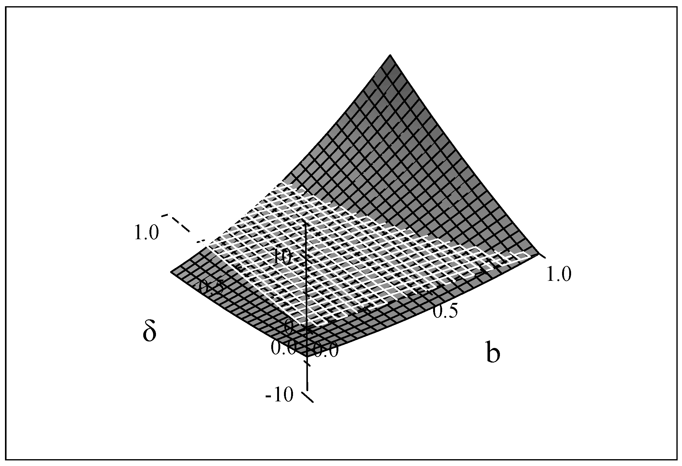
There is a trade-off between more intensive learning process under exclusivity and more varieties in the market under non-exclusivity. The “learning” effect refers to the increase in profits due to lower production costs, while the “product variety” effect refers to the increase in profits due to more variety in the market. We find that, when product differentiation is low (b is high), the “learning” effect dominates the “product variety” effect and firm B is excluded in period one and subsequently in period two. Intuitively, the more substitutable the products are, the less aggregate demand is foregone if product B is not present in the market and the lower cost is preferred.
An example of the difference in the present value of the profits,
, is useful to understand the equilibrium outcome. Note that, in
Figure 2, for high values of the product differentiation parameter (
), the present value of the profits under exclusivity is higher than under non-exclusivity; thus, one product is purchased by the retailer in equilibrium (since
). For a given level of the discount factor
(axis y), the difference in the present value of the profits starts out negative, for low values of
b, and turns positive as
b increases.
We examine now the properties of the equilibrium we have derived. First, we study the effect of learning-by-doing on the quantities produced and the profits. Then, we compare the quantities produced in the first period to the quantities produced in the second period. Consumer’s surplus and total welfare are examined separately in the next section.
Remark 1. As the learning parameter λ increases, all equilibrium quantities increase, the equilibrium profits in the first period decrease and the equilibrium profits in the second period and the present value of the total profits increase.
By directly differentiating the equilibrium quantities, we obtain that, for both products and for both periods, as the learning process becomes more intense, the quantities increase (
for
and
). Thus, total production under the learning-by-doing hypothesis exceeds the total production when there are no gains from experience (
), as is expected. Another implication is that the prices in the dynamic model are lower compared to the prices in the static one, where there is no learning and production costs do not reduce in time. By directly differentiating the relevant equilibrium expressions, available in the
Appendix A, we also obtain that the equilibrium profits in the first period decrease with
(
) but the equilibrium profits in the second period increase with
(
). Part of the retail profits should be sacrificed in the first period, in order to take advantage of the learning process in the second one. However, the present value of the profits always increase with
(
), which means that the dynamic model gives higher total profits compared to the static one.
Remark 2. The quantity produced in the first period is lower than the quantity produced in the second period, .
The marginal production cost in the first period is higher than the marginal production cost in the second one, which leads to higher prices in the first period () and lower quantities.
4. Consumer Surplus and Total Welfare
We have already demonstrated that, when products are close substitutes (), exclusivity emerges in the dynamic setting. Here, we study whether exclusivity is beneficial for the consumers and, thus, is welfare-enhancing as well. First, we compare the product prices among exclusivity and non-exclusivity.
Remark 3. When exclusivity is imposed by the retailer, the product prices in both periods reduce compared to the non-exclusivity case: , for .
When
, consumers face the positive effect of price reduction due to the more intense learning and the negative effect of reduction in the product variety available. Which effect dominates? Is exclusivity beneficial for consumers? We calculate the consumer’s surplus that accounts for prices and product variety and compare the two cases.
22
where the subscript refers to the time period.
The difference in the present value of the consumer’s surplus under exclusivity and non-exclusivity,
, is increasing in
b and there exists a unique and positive
b,
, such that
.
23 Above this critical
b, the difference in the present value of the consumer’s surplus is positive. Hence, the following proposition is proved.
Proposition 3. When products are close substitutes (b is positive and takes high values), consumer surplus is higher under exclusivity compared to non-exclusivity. The price reduction is more important than more variety for the consumers.
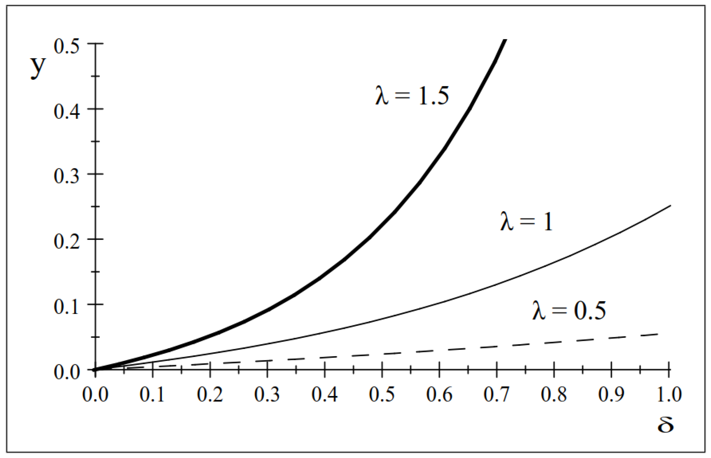
To prove that exclusivity is always beneficial for the consumers (when it is imposed by the retailer), it is sufficient to prove that the difference between the consumer’s surplus under exclusivity and non-exclusivity is positive when (that is, ). If this difference is positive at point , then it is positive for every , where exclusivity is imposed by the retailer. We have proved this argument and provide an example in the following figure for the difference in the consumer’s surplus.
In
Figure 3, we plot, for the various values of the discount factor
and the learning parameter
, the difference between the consumer’s surplus under E and NE divided by
when
. We call this expression
y, with
. This is equivalent to plotting
, since
. Observe that
y is positive and increasing in
and
; therefore,
is also positive. Thus, when exclusivity is chosen by the retailer, this also leads to higher consumer’s surplus compared to the non-exclusive case. Consumers prefer lower prices than more variety in the market when
. The difference in the consumer’s surplus increases with
and
. Since the discounted stream of profits and consumer’s surplus under exclusivity is higher than that under non-exclusivity, we have:
Proposition 4. When the retailer imposes exclusivity, total welfare is increased compared to the non-exclusive case.
6. The Role of the Intermediary
Finally, we study the role of the retailer in the learning process. Is the presence of such a retailer indeed necessary to intensify this process? Or can firms take advantage of the learning process equally efficiently without the downstream monopolist? First, we analyze the role of the retailer in the static model where there is no learning and then we study the dynamic model.
We compare the equilibrium outcome when the upstream firms sell their products to the final market indirectly, via the retailer, to the equilibrium outcome when the upstream firms distribute their products directly to the final consumers. When there is no intermediary, the outcome is the Cournot duopoly outcome with differentiated products and when a retailer exists, the outcome is the monopoly outcome (given in
Section 2). The key is the product differentiation parameter. When the products are substitutes (
) and there is no intermediary, the final prices and total profits are lower and the consumer’s surplus and total welfare are higher compared to the case where a retailer exists.
Remark 4. In the static model, when the products are substitutes, the presence of the intermediary hurts the market, since the retailer gains the monopoly profits by increasing the final prices and, thus, lowering the consumer’s surplus and total welfare. In contrast, when the products are complements, the role of the retailer in the market is positive, since it internalizes the externalities from the two complement goods. The prices are lower and the consumer’s surplus, profits, and total welfare are higher when there exists a retailer in the downstream level.
Then, we solve for the dynamic Cournot differentiated duopoly model with learning-by-doing technology and no intermediary. Both products are purchased in both periods and the equilibrium quantities for the first period are given by
26We compare these quantities to the quantities in our equilibrium model with the presence of the retailer:
27
and obtain that:
Remark 5. For we have , for we have and for we have
The presence of the intermediary intensifies the learning process when the two products are complements or when the products are close substitutes and exclusivity is imposed by the intermediary (i.e., ). The retailer coordinates the purchases of the two products and takes advantage of the learning process in a more efficient way compared to the case where upstream producers sell their products directly to the final consumers. The rate of learning is closer to the social rate of learning (for these parameter values of b) when there is an intermediary in the market.
7. Conclusions and Further Research
Learning-by-doing technologies can play a significant role in vertical chains. In this paper, we have examined how the learning-by-doing process affects the final market outcome in a vertical framework. Upstream firms produce differentiated products, either substitutes or complements, and the downstream monopolist sets the linear contract terms. The unit production cost of the upstream firms reduces with the accumulated production. We study how the dynamic interactions between upstream and downstream firms affect the exclusive dealing decisions in a two-period game. The existing literature has either examined vertical contracting without dynamic interactions due to learning effects or the learning-by-doing process in an oligopolistic industry without vertical considerations. Our paper is the first that studies a dynamic vertical foreclosure with learning-by-doing production technologies.
In the static model, both products are carried by the retailer. Exclusivity never arises in equilibrium, since final consumers like product variety. When we introduce dynamic considerations, the decision on imposing exclusivity depends on the product differentiation parameter. Close substitutability leads to exclusivity in the dynamic model, since the “learning” effect (leading to lower prices) dominates the “product variety” effect. In contrast, complementarity or a lack of close substitutability leads to an equilibrium where the retailer purchases both products in both periods. More varieties in the market are preferred to lower final prices. Consumer’s surplus and total welfare are also higher under exclusivity when it is imposed by the retailer compared to the case where exclusivity is not imposed (for example, due to regulatory restrictions). Therefore, exclusivity is welfare-improving. Nevertheless, the equilibrium rate of learning is not equal to the social optimum. A social planner would more often impose exclusivity and would further reduce the production costs in the second period compared to the retailer. Finally, when products are complements or close substitutes the presence of the retailer is necessary to coordinate the learning process.
There is often intense criticism for various exclusionary practices, which underlies economic policy decisions. Often, these practices are anti-competitive, but sometimes can be pro-competitive. In this paper, we characterize conditions under which exclusivity is beneficial for firms and consumers in a simple dynamic vertical framework with learning-by-doing production technologies. Our analysis enriches, thus, the set of results concerning exclusionary practices by highlighting the role of possible efficiencies through cost reduction.
Further research can, of course, shed light on additional aspects of the issue. In particular, our model is kept very simple regarding the allocation of bargaining power and endows the downstream firm with the ability to set linear wholesale prices. In a more complex setting, where the bargaining power may be more evenly distributed across the upstream and downstream firms, additional tensions will likely arise, partly reflecting results from earlier research on downstream ‘bottleneck’ models. If the upstream firms actively participate in the pricing decisions, the implicit coordinating role of the retailer would tend to be diminished, perhaps also leading to a reduced ability to motivate and exploit learning-by-doing. In parallel, competition between the upstream firms may tend to be more intense in the first stage of the game, so that they strategically improve their efficiency in the second stage, and partly benefit from this cost reduction. How the cost reduction versus product variety tension will play out in such a rich setting, and how profits will be allocated among the firms, would of course largely depend on the type of contracts that can be employed. Finally, it would be interesting to extend the present model by considering alternative demand specifications and learning-by-doing processes.


