
Cooperation and Coordination in Threshold Public Goods Games with Asymmetric Players

Abstract
:1. Introduction
- What is the impact of various forms of inequality on cooperation?
- How do people coordinate when group members differ among multiple dimensions?
2. Model
3. Results
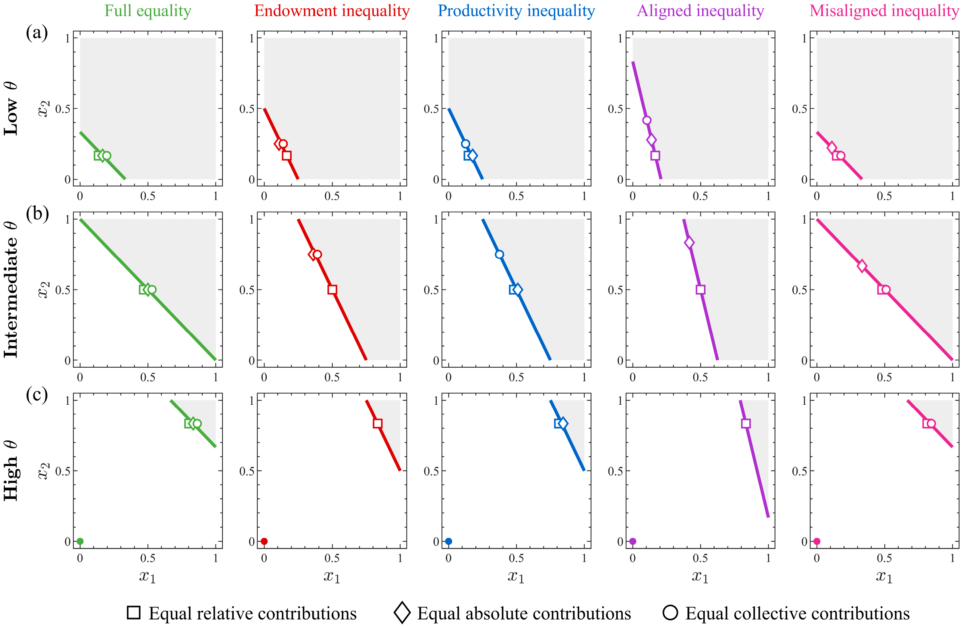
- (1)
- For relative contribution, if and if .
- (2)
- For absolute contribution, when there is endowment heterogeneity, i.e., and , for all . When there is productivity heterogeneity, i.e., and , if and if .
- (3)
- For collective contribution, for all . Furthermore, if .
4. Numerical Analysis
5. Concluding Remarks
Author Contributions
Funding
Data Availability Statement
Conflicts of Interest
Appendix A. Proof of Theorem 1
- (i)
- Existence conditions of a defective Nash equilibrium
- (ii)
- Cooperative Nash equilibria set and its existence condition
Appendix B. Proof of Theorem 2

- (i)
- When , each is an ()-dimensional convex polytope formed by vertices. Specifically, we define the following:
- (ii)
- When , we represent as and focus on the set . This set can be expressed as

| 1 | Dragicevic [10] theoretically studied a TPGG in the context of the option fund market and found that payoff inequality between buyers and sellers can undermine coordination efforts. |
| 2 | Dong et al. [19] considered a climate game with two types of players, in which rich (or poor) players have higher (or lower) endowment and emission reduction cost (i.e., low productivity). Their theoretical analysis and behavioral experiment based on specific parameters showed that the effect of multiple inequalities on coordination is generally more complex. More general discussion on NE in a climate game with heterogeneous players can be found in [19]. |
| 3 | We note that at an NE, the absolute contribution of player cannot exceed even if . Otherwise, this player can obtain a higher payoff by deviating to free-riding. Thus, this assumption does not affect the equilibrium structure of the game. |
| 4 | An alternative scenario is one in which players choose their strategies from a finite grid with sufficiently large . In this case, the cooperative NE set consists of finite number of equilibria, and for all () implies that there are more equilibria in which player contributes the most. |
References
- Cherry, T.L.; Kroll, S.; Shogren, J.F. The impact of endowment heterogeneity and origin on public good contributions: Evidence from the lab. J. Econ. Behav. Organ. 2005, 57, 357–365. [Google Scholar] [CrossRef]
- Heap, S.P.H.; Ramalingam, A.; Stoddard, B.V. Endowment inequality in public goods games: A re-examination. Econ. Lett. 2016, 146, 4–7. [Google Scholar] [CrossRef]
- Martinangeli, A.F.M.; Martinsson, P. We, the rich: Inequality, identity and cooperation. J. Econ. Behav. Organ. 2020, 178, 249–266. [Google Scholar] [CrossRef]
- Fisher, J.; Isaac, R.M.; Schatzberg, J.W.; Walker, J.M. Heterogenous demand for public goods: Behavior in the voluntary contributions mechanism. Public Choice 1995, 85, 249–266. [Google Scholar] [CrossRef]
- McGinty, M.; Milam, G. Public goods provision by asymmetric agents: Experimental evidence. Soc. Choice Welf. 2013, 40, 1159–1177. [Google Scholar] [CrossRef]
- Reuben, E.; Riedl, A. Enforcement of contribution norms in public good games with heterogeneous populations. Games Econ. Behav. 2013, 77, 122–137. [Google Scholar] [CrossRef]
- Kölle, F. Heterogeneity and cooperation: The role of capability and valuation on public goods provision. J. Econ. Behav. Organ. 2015, 109, 120–134. [Google Scholar] [CrossRef] [PubMed]
- Hauser, O.P.; Hilbe, C.; Chatterjee, K.; Nowak, M.A. Social dilemmas among unequals. Nature 2019, 572, 524–527. [Google Scholar] [CrossRef] [PubMed]
- Palfrey, T.; Rosenthal, H. Participation and the provision of discrete public goods: A strategic analysis. J. Public Econ. 1984, 24, 171–193. [Google Scholar] [CrossRef]
- Dragicevic, A.Z. Option fund market dynamics for threshold public goods. Dyn. Games Appl. 2017, 7, 21–33. [Google Scholar] [CrossRef]
- Wang, X.; Couto, M.C.; Wang, N.; An, X.; Chen, B.; Dong, Y.; Hilbe, C.; Zhang, B. Cooperation and coordination in heterogeneous populations. Philos. Trans. R. Soc. B 2023, 378, 20210504. [Google Scholar] [CrossRef] [PubMed]
- Rapoport, A.; Suleiman, R. Incremental contribution in step-level public goods games with asymmetric players. Organ. Behav. Hum. Decis. Process. 1993, 55, 171–194. [Google Scholar] [CrossRef]
- Alberti, F.; Cartwright, E.J. Full agreement and the provision of threshold public goods. Public Choice 2016, 166, 205–233. [Google Scholar] [CrossRef]
- Milinski, M.; Sommerfeld, R.D.; Krambeck, H.J.; Reed, F.A.; Marotzke, J. The collective-risk social dilemma and the prevention of simulated dangerous climate change. Proc. Natl. Acad. Sci. USA 2008, 105, 2291–2294. [Google Scholar] [CrossRef] [PubMed]
- Milinski, M.; Röhl, T.; Marotzke, J. Cooperative interaction of rich and poor can be catalysed by intermediate climate targets. Clim. Change 2011, 109, 807–814. [Google Scholar] [CrossRef]
- Tavoni, A.; Dannenberg, A.; Kallis, G.; Löschel, A. Inequality, communication, and the avoidance of disastrous climate change in a public goods game. Proc. Natl. Acad. Sci. USA 2011, 108, 11825–11829. [Google Scholar] [CrossRef] [PubMed]
- Feige, C.; Ehrhart, K.M.; Krämer, J. Climate negotiations in the lab: A threshold public goods game with heterogeneous contributions costs and non-binding voting. Environ. Resour. Econ. 2018, 70, 343–362. [Google Scholar] [CrossRef]
- Kline, R.; Seltzer, N.; Lukinova, E.; Bynum, A. Differentiated responsibilities and prosocial behavior in climate change mitigation. Nat. Hum. Behav. 2018, 2, 653–661. [Google Scholar] [CrossRef] [PubMed]
- Dong, Y.; Ma, S.; Zhang, B.; Wang, W.X.; Pacheco, J.M. Financial incentives to poor countries promote net emissions reductions in multilateral climate agreements. One Earth 2021, 4, 1141–1149. [Google Scholar] [CrossRef]
- Huang, Y.; Wang, X.; Zhang, B.; Dong, Y. Global emission reduction problem with heterogenous agents. J. Beijing Norm. Univ. Nat. Sci. 2023, 59, 806–811. [Google Scholar] [CrossRef]


| Threshold | NE | ||||
|---|---|---|---|---|---|
| Full equality | |||||
| Endowment inequality | |||||
| Productivity inequality | |||||
| Aligned inequality | |||||
| Misaligned inequality | |||||
Disclaimer/Publisher’s Note: The statements, opinions and data contained in all publications are solely those of the individual author(s) and contributor(s) and not of MDPI and/or the editor(s). MDPI and/or the editor(s) disclaim responsibility for any injury to people or property resulting from any ideas, methods, instructions or products referred to in the content. |
© 2023 by the authors. Licensee MDPI, Basel, Switzerland. This article is an open access article distributed under the terms and conditions of the Creative Commons Attribution (CC BY) license (https://creativecommons.org/licenses/by/4.0/).
Share and Cite
An, X.; Dong, Y.; Wang, X.; Zhang, B. Cooperation and Coordination in Threshold Public Goods Games with Asymmetric Players. Games 2023, 14, 76. https://doi.org/10.3390/g14060076
An X, Dong Y, Wang X, Zhang B. Cooperation and Coordination in Threshold Public Goods Games with Asymmetric Players. Games. 2023; 14(6):76. https://doi.org/10.3390/g14060076
Chicago/Turabian StyleAn, Xinmiao, Yali Dong, Xiaomin Wang, and Boyu Zhang. 2023. "Cooperation and Coordination in Threshold Public Goods Games with Asymmetric Players" Games 14, no. 6: 76. https://doi.org/10.3390/g14060076