1. Introduction
The issue of scarcity of water resources has been a topic of extensive discussion among scholars, the public, and policymakers, due to its potential impact on individual activities and on agricultural and industrial production. Public opinion, and the views of the other actors mentioned, argue that regulating the withdrawal of water, particularly for productive activities, is the key to managing this issue. However, managing this problem, along with the challenge of not treating natural resources as capital, has made it crucial to research and develop efficient rules for allocating water among competing uses over time and space [
1]. In recent years, there has been increased interest in resolving conflicts related to water extraction, especially in agricultural and industrial contexts, and various quantitative methods have been proposed to address these issues. In particular, the literature proposes several models based on game theory, where the main purpose is to study the existence, and possible properties, of optimal solutions in relation to the extraction and consumption of water resources.
A first paradigmatic theoretical work in the field of water management is represented by the article proposed in [
2], where the authors analyze the inefficiency of private exploitation of water resources, caused by a pumping cost externality and a strategic externality due to competition between farmers. In particular, the authors present a first “estimate” of this inefficiency, comparing socially optimal exploitation (optimal control) with private (competitive) exploitation, using data from the Pecos River basin in New Mexico. The authors applied the following assumptions: (i) farmers are “short-sighted” and choose their extraction rate to maximize their current profits, while optimal exploitation is achieved by maximizing the present value of the aggregate profit stream; (ii) linear water demand and average extraction cost, independent of extraction rate, linearly decrease with respect to groundwater level. With their assumptions in place, the authors showed that, if the storage capacity of an aquifer is relatively large, the difference between the two systems is so small it can be ignored. Focusing on the study of inefficiency in the exploitation of water resources, and using the game theory approach, the author in [
3] determined both the open-loop Nash solution, where it is assumed that all farmers commit, from the initial period, to constant rates of pumping the water resource, and the feedback Nash solution, where farmers adopt pumping strategies dependent on the water reserve (a more realistic assumption). The author then showed how the open-loop equilibrium manages to capture only the externality of pumping costs, while, in the feedback approach, strategic externalities also emerge. Assuming the concavity of the objective function of the problem, the model proposed by [
4] shows that the feedback solution increases inefficiency with respect to a socially optimal outcome (derived from optimal control). Subsequently, in [
5,
6], differential games, studying open-loop and feedback scenarios over an infinite planning horizon, were proposed and used to analytically determine “social optimum” solutions. The results emerging from the analysis coordinated with those observed in [
2]. In fact, the analysis of the model showed that strategic behavior increases groundwater exploitation compared to the open-loop solution, but, in the case of high groundwater storage capacity, the difference between the social optimum and private extraction is negligible. More recently, [
7] introduced ecosystem damage caused by pumping and showed how these environmental externalities can substantially change the results previously obtained in the literature. In particular, their analysis highlights, both theoretically and empirically, the importance of policies in water management, as well as the potential role of stakeholder cooperation. In addition, an empirical comparison was conducted between two aquifers in Spain: the western aquifer of La Mancha, which is severely mismanaged, and the eastern aquifer of La Mancha, which is oriented towards sustainable management.
By reconsidering the results of [
2], several papers have recently addressed the problem of how a public agency allocates water from (one or more) aquifers to different users (e.g., farmers and municipalities), in order to ensure the collective welfare of users and sufficient drainage to preserve the ecosystem, as discussed in [
8,
9,
10]. Similarly, [
11] developed a differential game to determine the efficient extraction of the aquifer resource in overlapping generations framework (OLG) modeling. In such a framework, both intragenerational and intergenerational competitions in exploiting the resource were considered and the authors computed feedback equilibria in order to determine the optimal extraction rates for young and old agents coexisting in the economy. The effects of legal and illegal firms’ actions, and the contribution of taxes and penalties imposed by public authorities, are analyzed in [
12,
13,
14,
15]. A crucial issue discussed in the literature is also the allocation of water among multiple users who usually have a higher water requirement than the quantity available. On this topic, [
16] defined a modified cooperative game for the sharing of additional net benefits under a scenario having water demand management. Their results suggest that cooperation among water users may yield more net benefits, and a water demand management plan can lead to further increase in the aggregated net benefits by means of water transfers from less productive users to more productive ones. The work in [
17] addresses a similar issue, using a dynamic Nash bargaining approach, and in [
18] a static leader–follower game is analyzed, in which two competitive water resource supply chains derive their optimal decision strategies under different power structures.
Parallel to the above models, the literature has recently focused on studies related to how a water supplier may determine the price of the resource and how users may react to such decisions. On this topic, an interesting contribution is given by [
19], wherein the authors consider a vertical supply chain consisting of a water provider and a consumer (municipality). The inherent conflicts over stocks and supply costs that emerge among the parties in the water supply chain are modeled as a zero-sum stochastic differential game. In addition, refs. [
20,
21] address the problem of dynamic interaction between two firms committed to providing water supplies within a limited time horizon.
In this work, we consider an agency (public or private) that sells and distributes water to an individual user (whether domestic, agricultural or industrial). The seller aims to maximize revenue, minimize costs, take into account the well-being of users, and preserve the necessary availability of the resource for the future. The agency defines the price at which water is sold. It can vary over time and depends on the availability of water in the generic basin considered. The user adjusts the demand for water in response to its price and his or her current (seasonal) need. The user does not observe the water stock but only the price and, therefore, behaves myopically. The seller, on the other hand, is farsighted because he or she is also concerned with maintaining optimal water availability for the future. In the model, we also assume that two different pricing schemes are possible: (i) the classic linear scheme; (ii) a block scheme, where the user, if requesting water above a certain threshold, pays a higher price for the additional quantity; (iii) a more general scheme, which takes into account increasing marginal prices. Regarding all the proposed price schemes, we characterize the open-loop Stackelberg equilibrium of the game in order to investigate what the optimal water demand of the user is in response to the tariffs applied and to understand if either the block pricing scheme or the convex one is preferable in terms of linear pricing. The formal analysis is supported by a series of numerical simulations able to capture interesting properties of the solutions. Specifically, the numerical exercises enable observation of the different ways in which both the seasonality of the basin’s recharge capacity and the seasonal component in the agent’s preferences with respect to water may affect the optimal price and the dynamics of purchasing the water.
The rest of the paper is organized as follows.
Section 2 presents the model. In
Section 3, two different tariff schemes are discussed. In
Section 4, the open-loop Stackelberg equilibrium is characterized. In
Section 5, numerical simulations are provided and some properties of the solution and policy implications are discussed.
Section 6 concludes. All proofs are provided in the
Appendix A.
2. The Model
Consider an agency (public or private) that sells water extracted from a generic basin, to a user, whether a company or a private individual, for domestic needs.
1 At instant,
t, the user requests the amount,
, that depends both on the user’s needs (which can also be seasonal) and on the price of the water itself, and receives from the agency the amount,
, with
. The water stock at time
t is given by
, with
, where
is the capacity of the aquifer. The capacity depends not only on consumption, but also on the natural recharge capacity
, where
is a continuous function.
The seller incurs two types of costs: fixed costs and costs which may depend, as in the case of groundwater management models, on the available water reserve. Specifically, we assume
to be the cost of extracting water per unit volume at time
t,
,
.
2 The unit cost is
if the aquifer is completely full, increases as the water stock decreases, and is at a maximum when the aquifer is empty. In addition, we consider the time horizon established by the duration of a contract, normalized to 1. Therefore, it is
.
The user pays the supplier the amount
to buy the amount of water
W at the time
t. The function
Z is assumed to be continuous with respect to
t and
W and increasing in
W.
The payoff of the supplier is its net income at time
tThe buyer derives a utility
from the purchase of water, which can be seen as a kind of production function. Specifically,
depends both on the volume of water purchased and on the season, being the time
t.
3 We assume that
where
and
is a differentiable and strictly increasing concave function.
The payoff of the buyer at time
t is
The dynamics of the water stock is given by
where
The game is played in the following way:
The agency announces the tariff scheme of water .
The buyer, having observed the tariff scheme, but not , decides the quantity of water to demand, maximizing the present value of its net income.
The agency supplies the buyer with the quantity of water .
The agency makes its choices to maximize the present value of its overall net income. Moreover, it can also take the welfare of the buyer into account (which is reasonable when the seller is a public agency). Since the time horizon of the model is short, we neglect any discount factors.
3. Tariff Scheme and Water Demand
The seller can choose between different pricing schemes. There is much literature on the subject and a vast typology of schemes adopted in practice. The simplest is to charge each user a fixed price per unit of volume purchased. However, in order to discourage the excessive, and sometimes inappropriate, use of a scarce commodity, such as water, the literature proposes tariff schemes that make the user pay a marginal price that increases with the quantity of water purchased. The best known of these schemes consists of the so-called block tariffs, whereby the unit price of water is established for brackets of volumes of water purchased and increases as consumption increases (see, for example, [
25]). The user does not observe, and does not care about, the water stock and, therefore, maximizes his or her instant payoff. Hence, the user acts myopically.
Assume that the function
is strictly increasing and convex with respect to
x and
. Moreover, to ensure the existence and uniqueness of a positive water demand, we request
The first-order condition applied to the payoff
gives
Assumption (5), concavity of and convexity of ensure that Equation (6) has a unique positive solution
Note that, as expected, increases as the coefficient increases.
Special Pricing Schemes
Remark 1. Given and we have the following:
If the block threshold is large enough, then it is optimal to buy a quantity of water at the cheapest price and the block tariff gives exactly the same solution as the linear pricing scheme.
If the block threshold is neither too high nor too low, then it is optimal to buy a quantity of water equal to at the cheapest price and the block tariff reduces the demand for water compared with the linear pricing case.
If the block threshold is small enough, then it is optimal to buy a quantity of water paying the quantity at the lower price and the excess quantity at the higher price; moreover, the demand is lower compared with the linear pricing case.
In any case, the reduction in demand decreases as the threshold increases.
- 3.
Convex tariffs. A more general setting to account for scarcity is to introduce increasing marginal prices through the convex function
4 The optimal demand
solves the equation
decreases as or increase.
Remark 2. To improve our understanding of the results, it pays to specialize the utility function ψ. Assume 4. The Open-Loop Stackelberg Equilibrium
The model described above naturally defines a Stackelberg game with two players, in which one player (the leader) moves first and the second (the follower) moves in turn knowing the opponent’s move, see [
26].
In the game we define, the time horizon is equal to the duration of a contract. At the beginning of the period, the supplier communicates the price of the product (possibly time-dependent) and undertakes to respect it for the entire duration of the contract. In this case, the suitable strategy is the open-loop one.
5 We look for interior solutions, which means, among other things, that the water basin never empties during the time horizon. Therefore, in this Section we assume the market clearing condition
to be satisfied. The game is a two-stage leader–follower game. At the first stage, the agency determines its tariff scheme
, maximizing its overall payoff
J, which is given by
subject to the state variable constraints (3) and (4).
and
are defined in (1) and (2), respectively.
The payoff J of the agency is the sum of three contributions: the first addendum is given by the current value of the agency’s profits (revenues minus costs); the second addendum takes into account the overall payoff of all users and is due to the social role that a public agency carries out; the third addendum (scrap value) takes into account the value for the agency of the water stock at the end of the time horizon considered. The coefficient weighs the social role of the agency. In particular, corresponds to the case of a totally private agency with no social obligations. We assume that the scrap value function is an increasing function and .
We solve the game by backward induction. At the second stage, the buyer, having observed the price scheme , determines the quantity of water to demand. As seen in the previous section, each buyer solves, instant by instant, a static maximization problem (acting myopically). From the previous section, we have the following proposition.
Proposition 1. The optimization problem of the buyer has a unique solution , given by the unique positive solution of the equation At the first stage, the seller, foreseeing the buyer’s response, solves the following optimal control problem
subject to the state variable constraints (3) and (4). In what follows, we assume that the function
is given by (8). Moreover, we need to analyze separately the special tariff schemes introduced in
Section 3.
4.1. Linear Pricing Schemes
The following proposition holds:
Proposition 2. If the agency adopts a linear pricing strategythen the optimal unitary price is The corresponding optimal demand function is is a solution of the algebraic Equation (16),where Remark 3. As expected, decreases as ρ increases. The more the agency cares about the buyer’s payoff, the less it charges for the water. is monotone decreasing in .
4.2. Block Tariffs
Assume that the seller adopts the following block tariff scheme:
Note that (17) boils down to the linear pricing scheme in the particular case .
The following proposition holds:
Proposition 3. If the agency adopts the block tariff strategy (17) then it is optimal to choose . The optimal prices and demands are given in (14) and (15), respectively.
Remark 4. Proposition 3 states that a block pricing scheme is never optimal compared to a linear pricing scheme. This contrasts with the widespread practice in many countries of applying block tariffs for urban water consumption.
4.3. Convex Tariffs
The following proposition holds.
Proposition 4. If the agency adopts a convex tariff strategythen the optimal function is The optimal water demand is is a solution of the algebraic Equation (19),where Remark 5. It can be observed that decreases in time, while the behavior of over time depends on seasonal factors ϕ and R.
5. Numerical Results
This section is devoted to a discussion of the numerical exercises and the implications of the analytical results obtained in
Section 4. To perform the following numerical simulations, we applied the following specifications for the natural recharge,
, and the seasonal component of the buyer’s preferences,
:
where
,
and
.
6 All the numerical exercises were performed, without loss of generality, by neglecting to consider the scrap value and applying the following parameter set:
.
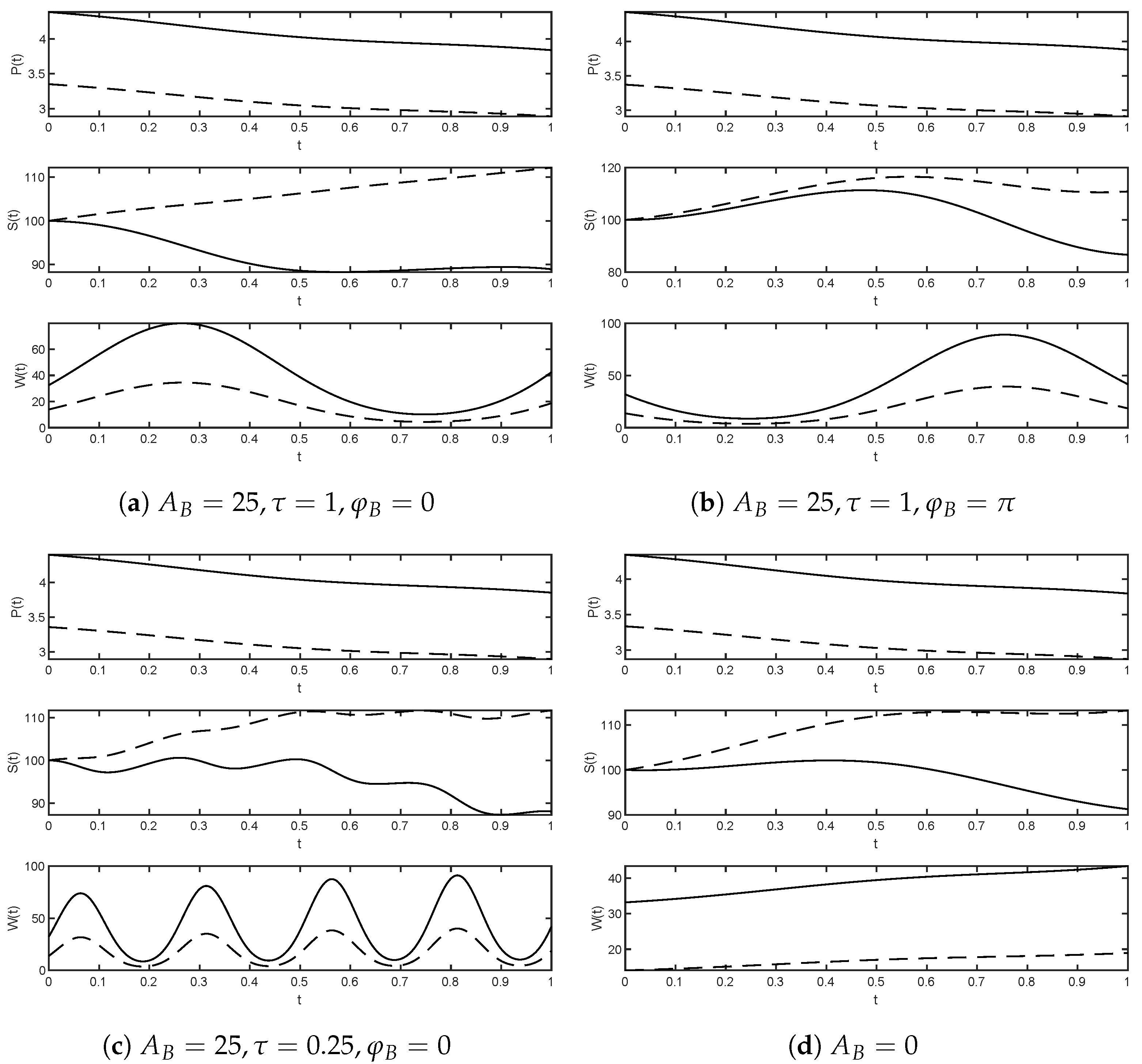
Assuming the seasonality in the basin recharge to be fixed, numerical simulations make it possible to capture the role of the seasonal (or, at least, cyclical) component in the preferences that the buyer has with respect to the water purchase. In fact, we can observe that seasonality had a remarkable effect on the dynamics related to price, optimal demand, and level of water present in the basin along time horizon considered. Specifically, Panel (a) in
Figure 1 shows that, if the cyclical phases of recharge and preference are synchronized (
), the recharge capacity was simultaneously eroded by increasing demand for the resource. Consequently, in the phase where both recharge and demand stood out at low levels, the basin level remained trapped at low levels of available water. On the contrary, as Panel (b) of
Figure 1 displays, when seasonality of recharge and preference had asynchronous behaviors (
) the basin alternated between a phase of resource accumulation (which was not immediately eroded) and a subsequent phase of discharge during the period when the buyer’s preference toward water increased and, consequently, demand increased. Panels (c) and (d) in
Figure 1 then show the dynamic events in two particular cases. Panel (c) shows what happens to the variables in the case where preferences with respect to water undergo multiple intraperiod fluctuations (
), while panel (d) observes the dynamic scenario related to the case where the buyer’s preference with respect to the resource is constant (
). In the latter case, due to the structure of the model, the demand dynamics increased, while those of the basin level ended up decreasing to rather low levels, due to an inability of the recharge to contain the increasing demand for water. In all the panels of
Figure 1, we observe continuous curves (related to the case with a linear tariff) and dashed curves (related to the case with a convex tariff). The convex tariff always guaranteed higher levels for the aquifer. This was due to the clear disincentive action (with respect to excessive water use) that the convex tariff had on the buyer. In fact, it guaranteed lower levels of demand (and price) than those in the linear case and, consequently, the possibility of a basin with more available resource at any
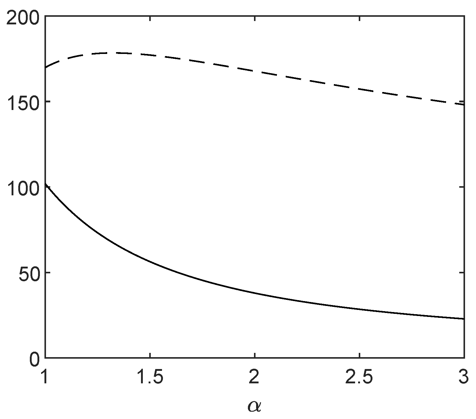
tThe role of the convex tariff is also highlighted in
Figure 2, where the payoffs
J (continuous curve) and
(dashed curve) are shown. The presence of a convex tariff and an increasing degree of convexity reduced the value of the seller’s payoff
J, which would be at a maximum in the linear price case (i.e.,
). Conversely, the convexity of the pricing scheme exhibited an ambiguous role on the buyer. Indeed, for values of
just greater than 1 the buyer’s payoff
increased before gradually decreasing as
increased toward large enough values.
6. Conclusions
In this article, we studied a leader–follower differential game with a finite time horizon. The leader (the agency) determines the selling price and the follower (a single buyer) reacts by requesting the resulting amount of water. We calculated the Open-Loop Stackelberg equilibrium assuming that the user demand was fully satisfied (interior equilibrium). We analyzed different tariff schemes: linear tariffs (the price paid is a multiple of the volume of water purchased), increasing block tariffs (the unit price is lower for quantities of water that do not exceed a fixed threshold), and convex tariffs, which take into account increasing marginal prices. Further, through numerical simulations, we highlighted the effects that both the tariff’s convexity and the seasonality of the buyer’s preferences had on the dynamics of water price and demand and, especially, on the levels experienced by the basin along the time horizon considered. In particular, we showed how synchrony and asynchrony between the cyclicality in the basin recharge and the seasonality in the buyer’s need for water can dictate very different dynamics and final aquifer levels. In addition, we observed that, in the presence of a large number of fluctuations in the buyer’s preferences (and, thus, in the buyer’s demand for water), the basin underwent the same kind of fluctuations but, thanks to the action of natural recharge, could maintain acceptable levels to satisfy future water demand.


