Deterrence, Backup, or Insurance: Game-Theoretic Modeling of Ransomware

Abstract

In this paper, we present a game-theoretic analysis of ransomware. To this end, we provide theoretical and empirical analysis of a two-player Attacker-Defender (A-D) game, as well as a Defender-Insurer (D-I) game; in the latter, the attacker is assumed to be a non-strategic third party. Our model assumes that the defender can invest in two types of protection against ransomware attacks: (1) general protection through a deterrence effort, making attacks less likely to succeed, and (2) a backup effort serving the purpose of recourse, allowing the defender to recover from successful attacks. The attacker then decides on a ransom amount in the event of a successful attack, with the defender choosing to pay ransom immediately, or to try to recover their data first while bearing a recovery cost for this recovery attempt. Note that recovery is not guaranteed to be successful, which may eventually lead to the defender paying the demanded ransom. Our analysis of the A-D game shows that the equilibrium falls into one of three scenarios: (1) the defender will pay the ransom immediately without having invested any effort in backup, (2) the defender will pay the ransom while leveraging backups as a credible threat to force a lower ransom demand, and (3) the defender will try to recover data, only paying the ransom when recovery fails. We observe that the backup effort will be entirely abandoned when recovery is too expensive, leading to the (worst-case) first scenario which rules out recovery. Furthermore, our analysis of the D-I game suggests that the introduction of insurance leads to moral hazard as expected, with the defender reducing their efforts; less obvious is the interesting observation that this reduction is mostly in their backup effort.

1. Introduction

Ransomware is a major type of cybercrime that organizations face today. It is a form of malicious software, or malware, that encrypts files and documents on a computer system, which can be a single PC or an entire network, including servers. Victims are often left with little choice: to regain access to their encrypted data without a decryption key, they have to either pay a ransom to the criminals behind the ransomware or try to restore from data backup (or rebuild the system in the absence of backup). Various real-world examples of these scenarios are given in the next section when describing our models. It is more than a mere nuisance for companies, even small ones, if vital files and documents, networks, or servers are suddenly encrypted and inaccessible. Even worse, a successful ransomware attack is often publicly and brazenly announced by the criminal, making it known that one’s corporate data is being held hostage, adding pressure on the victim to resolve it quickly, which almost always means swift payment.

The recent two years of a global pandemic saw a sharp increase in ransomware attacks. In the first half of 2022, there were 236.1 million ransomware attacks worldwide. Through 2021, there were 623.3 million ransomware attacks globally, an increase of 105% over 2020 [1]. According to astra [2], 2123 cyber insurance claims in 2022 were due to ransomware attacks.

This increase in threats has also accelerated discussion by the insurance industry on whether and how to provide ransomware coverage. The court ruling on G&G Oil Co v. Continental Western Insurance Co. by the Indiana Supreme Court [3] further brings into sharp focus the importance of much-needed clarity in insurance coverage pertaining to ransomware payment and will likely spur more development on this front.1

In this study, we are interested in understanding what firms can do to reduce damages from potential ransomware attacks and the role that ransomware insurance can play. We do so by modeling and analyzing the strategic decision making in a ransomware attacker-defender-insurer ecosystem. Specifically, we introduce two sequential games.

The first, attacker-defender (A-D) game models the interactions between an attacker (their action being ransom demand) and a (risk-averse) defender (their actions including protection, backup, pay or not pay, as detailed below).2 This is formulated as a complete information game, where the attacker is assumed to know the defender’s data value, risk attitude, cost of general protection, cost of data backup, and cost of data recovery. This puts the attacker in a rather strong position, and allows us to examine their best possible strategy in terms of ransom demand; it also serves as a worst-case scenario for the defender.

The second, defender-insurer (D-I) game models the interactions between a (risk-averse) defender who is seeking ransomware insurance and a risk-neutral insurer who determines the policy terms of the insurance. This is formulated as a complete information game between the defender and insurer, with the attacker being a non-strategic third party (whose ransom demand is input to the game model). This model treats the ransomware attack as a constant existence much like ambient noise; this is justified by the fact that many such attacks are not targeted and the ransom amount is set based on empirical knowledge of past successes rather than on individual victims’ specific information.3 This modeling choice also allows us to focus on the contractual relationship between the defender and insurer and better understand the impact of insurance.

Since both are sequential, multi-stage games, the solution concept we employ is the subgame perfect equilibrium [5]. The equilibrium outcome of the A-D game (ransom demand) is used as input to the D-I game as the defender’s outside option, since insurance purchase is assumed to be voluntary. However, this setup is in general not equivalent to a three-way, attacker-defender-insurer game, which remains an interesting direction of future research.

There is a very rich literature on game theoretic attacker-defender models for generic attack types, see e.g., [6,7,8], and an emerging literature of game theoretic analysis of ransomware attacks [9,10,11]. Laszka et al. [9] propose a two-stage model that considers backup effort on the defender’s part, but without the possibility of recovery failure or deterrence effort. Baksi and Upadhyaya [10] demonstrate the conditions the defender is in a position of advantage to successfully neutralize the attack, but neither backup nor deterrence effort is considered. Li and Liao [11] propose a different model that the attacker may sell the stolen data rather than publish the data for free. Researchers also draw heavily from game-theoretic literature on the more traditional form of kidnapping for ransom to obtain insights into its digital parallel, ransomware. Examples include [12,13] which invoke the use of a negotiation model, which is critical to the successful recovery of a kidnapping victim in the traditional form of ransom, and [14], which examines the impact of cooperative (negotiate or pay) vs. competitive (avoid payment) strategies on the attacker and the victim.

Research on ransomware insurance is much more limited, despite an increasing literature on ransomware and its economic, vendor, and consumer impact, see e.g., [15], and an increasing literature on cyber insurance in general, see e.g., [16,17,18,19]. In particular, [16] presents a network model where the insurer is attack aware, but the insurance contracts are not designed specifically for ransomware coverage. We will further discuss points that distinguish our study from prior works in the next section.

The remainder of the paper is organized as follows. In Section 2 we provide a general overview of our models and summarize the main findings. In Section 3, we introduce the A-D game and analyze the properties of the subgame perfect equilibrium. In Section 4, we introduce the D-I game and study its equilibrium and solution methods. In Section 5, we use numerical experiments to visualize equilibrium strategies for both the A-D and D-I games and summarize empirical findings. We conclude and discuss future work in Section 7.

2. Model Overview and Main Findings

We will assume that the attacker is financially driven, and the objective behind the attack is monetary gain. This rules out the case where the attacker simply seeks to destroy data without any real intention of releasing the decryption key, as was the case in the NotPetya malware attack in June 2017 [20], masquerading as ransomware but designed to cause maximum damage.

We will assume that the cost of launching a ransomware attack is negligible, which eliminates “attack or not attack” as a decision for the attacker: if it costs nothing, then the attacker will always launch an attack. In reality, many ransomware attacks are indeed very low cost, such as through the attachment in a spam email, see e.g., CryptoLocker [21], Avaddon [22], and can be easily automated to target a large population. Since our focus is on the interaction between a single attacker and a single defender (one of a large number of defenders or would-be victims), it seems reasonable to assume that the attacker does not dwell on this decision for each individual target.

We will also assume there is no negotiation post-attack; in other words, once an attack is successful, a ransom demand is issued, which is either paid in full or turned down. Post-attack negotiation is a crucial part of kidnapping for ransom and arguably the most important mechanism in the successful recovery of the kidnapping victim [23]. Ransom negotiation has been modeled in the case of ransomware attacks in the literature, see e.g., [12]; however, this so far seems to be rare in practice. One possible reason is again that a typical attacker targets a large number of entities at the same time, which makes negotiation impractical. At the same time, ransom demands are typically not as high as in real kidnappings (e.g., $189 in the AIDS Trojan case [24], $750 in the CtyptoLocker case [21], $500–$1500 in the Hermes case [25], or $35K for an oil and gas company such as G&G [3]), which encourages payment in full or signals lack of room for negotiation.

It is worth noting that the more recent Colonial Pipeline case [4], where the victim promptly made $4.4M in ransom payment, may be ushering in a new era in ransomware attacks: we may start to see increasingly targeted, costly attacks demanding much higher ransom payment; we may also start to see more involvement of law enforcement agencies in the payment decisions.

There are a few key elements in our model.

1.

The first is the separation of data backup effort from general protection measures. This separation is consistent with defenses generally recommended to protect against ransomware attacks [26], and gives the defender two types of actions or efforts to invest in prior to an attack. General protection measures (e.g., employee training against social engineering, software upgrades, and vulnerability patching, etc.) serve the purpose of deterrence, and make an attacker’s effort less likely to succeed. Data backup serves the purpose of recourse, in the event a ransomware attack is successful, so that the defender may have the ability to recover their data (but recovery is not guaranteed so there is a residual risk) without having to pay the ransom. As an example, Fujifilm recovered from a ransomware attack by restoring their network from backups [27].

2.

The second is a recovery cost to capture the cost that the defender incurs in delaying ransom payment while trying to recover their data. This models the cost of business interruption following an attack until the crisis is resolved. This combined with the previous feature gives the defender an additional decision point after an attack succeeds: they can decide to pay right away or try to recover their data, knowing that the recovery may ultimately fail, in which case they may be forced to pay the ransom, or rebuild the system in the absence of backup. As an example, after refusing to pay a ransom demand of $52,000, the city of Atlanta eventually spent $2.6M to rebuild their system [28]. In another example, the malware Jigsaw deletes files gradually as time passes, effectively increasing the victim’s cost when delaying payment [29].

Our main results are summarized below.

2.1. Main Findings from the Attacker-Defender (A-D) Game

Since the attacker is strategic in this game, they will seek to achieve a higher expected monetary gain. It seems obvious to assume that the attacker will prefer a higher ransom. However, a high ransom will push the defender to invest in backup and attempt to recover data first instead of paying ransom immediately. If so, the attacker is then faced with an increased likelihood of receiving nothing (if data recovery is successful). On the other hand, a lower ransom may persuade the defender to pay without trying to recover data, which removes the recovery cost associated with data recovery as well as the possibility of failure. Our analysis of the A-D game suggests that the equilibrium point is one of three types summarized below.

1.

The attacker demands a ransom equal to the data value in case of a successful attack. The defender pays immediately without having invested anything in data backup. Paying ransom immediately is a common case in the real world. For example, the Colonial Pipeline CEO Joseph Blount agreed to pay a $4.4 million ransom to DarkSide after the company was attacked [4]; the report reveals that Blount decided to pay ransom almost immediately.

2.

The defender invests zero4 or positive effort in data backup, but nevertheless pays ransom immediately. In response, the attacker’s ransom demand is lower than the data value, incentivizing the defender to not attempt data recovery. In this case, data backup serves as a credible threat so as to lower the ransom demand, but is not actually used.

3.

The defender invests zero or positive effort in backup and attempts data recovery, paying the ransom only if recovery fails; at the same time, the attacker charges a ransom equal to the data value. This case occurs far less often than the other two cases and only happens when the defender has low risk-aversion and has a relatively low cost of recovering data.

Note that the first case is a worst-case scenario for the defender, allowing the attacker to charge the highest possible ransom knowing that the defender will have no choice but to pay. This case occurs when the recovery cost is relatively large. In comparison, in the other two cases, the defender uses data backup to lower the attacker’s profit and their own expected loss, either using backup as leverage to force the attacker to charge a lower ransom, or to leave them empty-handed by recovering from backup. The second case occurs when the recovery cost is in the middle range, and the third case is when the recovery cost is low. We observe that a more risk-averse defender is more likely to rule out recovery, due to fear of recovery failure, which makes them bear both the recovery cost and the ransom demand. It is noteworthy that the highest backup effort occurs in the second case, which is only leveraged as a threat but never used. Our numerical results show that a more risk-averse defender is more likely to fall into the second case, i.e., making a compromise by paying a lower ransom directly to the attacker, while lower risk-aversion means one is willing to pay the highest ransom (either immediately or after a failed recovery attempt).

2.2. Main Findings from the Defender-Insurer (D-I) Game

In this game, the attacker is a non-strategic third party but serves as the defender’s outside option (outside the insurance contract) to ensure that the defender’s utility is not lower after purchasing insurance. The non-strategic assumption comes from our belief that whether the defender is insured or not is generally not public knowledge. Our main findings in this game are:

1.

The introduction of insurance causes the defender to invest less in efforts overall. This manifestation of moral hazard has been observed in other insurance models, where the insureds lower their effort once they have transferred all or part of their risk to the insurer. The more interesting observation, however, is that this effort reduction is much more concentrated on backup than on deterrence. In particular, we observe that numerically, the backup effort is almost completely abandoned under insurance, while some investment in deterrence remains, albeit at a reduced level. This is despite the fact that the insurer (under an optimal policy) covers almost the entire effort cost by the defender (in the form of a premium discount) and covers all losses upon a successful attack.

2.

The defender’s utility remains the same inside or outside insurance, and the attacker’s utility increases, due to lower levels of backup and deterrence efforts. The insurer’s profit (whenever it is positive) is essentially drawn from taking advantage of the defender’s risk-aversion. Our numerical results support this claim by showing that the insurer’s profits increase as the defender becomes more risk-averse.

3.

The introduction of insurance does not significantly alter the defender’s decision making in dealing with the attacker (in terms of paying vs. recovering), but only their effort amount.

3. The Attacker-Defender (A-D) Game: Model, Analysis, and Results

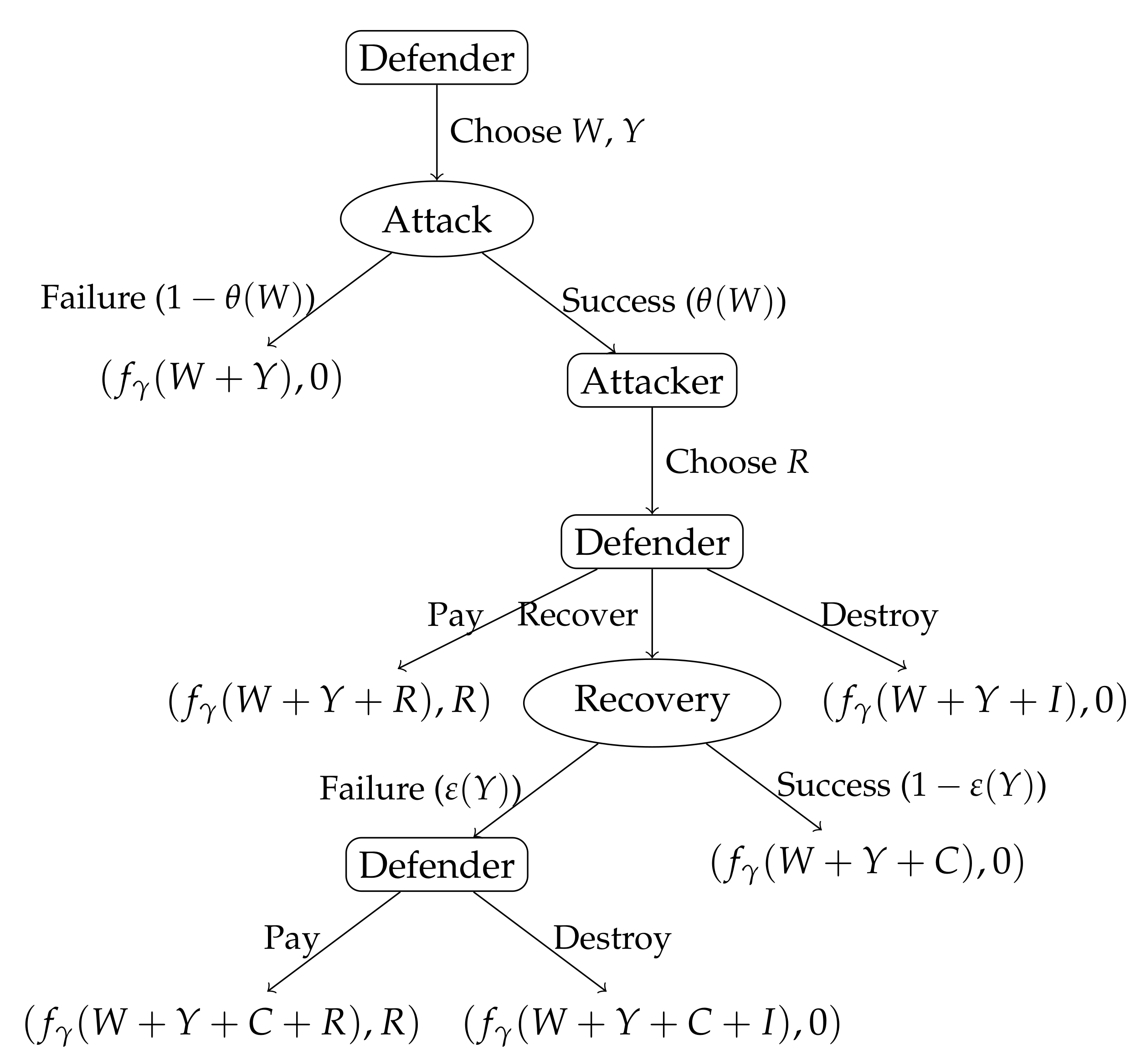
In this section, we introduce and analyze the attacker-defender (A-D) game. This game involves two players, an attacker and a risk-averse defender, making sequential moves over multiple stages. A diagram illustrating this multi-stage game and all its possible outcomes is given in Figure 1, where the two players’ utilities, denoted by $U_a$ and $U_d$, are written out and explained in more detail below.

results=[text centered,draw=none] stages =[rounded corners,text centered, draw = black] pending=[ellipse, text centered,draw=black] arrow = [->=stealth]

The defender’s utility $U_d$ takes the form $U_d=f_{\gamma }\left(x\right)$, where x is the total cost borne by the defender and $\gamma >0$ represents the risk attitude of the defender, with a larger $\gamma$ indicating more risk-aversion.

The defender holds data of value $I>0$. The sequential game consists of the following four stages.

• Stage I

The defender chooses a deterrence effort $W\ge 0$ (such as investing in an effective firewall, employee education against phishing campaigns, etc.), as well as a data backup effort $Y\ge 0$.

• Stage II

The attacker launches an attack with a success probability of $\theta \left(W\right)$, a non-increasing and convex function of the defender’s deterrence effort W.

We will denote by ${\theta }_o=\theta \left(0\right)$ the attack success probability under zero protection effort, and by ${\theta }_{\infty }={lim}_{W\to \infty }\theta \left(W\right)$ the minimum achievable attack success probability.

• If the attack fails, then the game ends with $U_a=0$ and $U_d=f_{\gamma }(W+Y)$.
• If the attack succeeds, then the attacker gains access to and encrypts the defender’s data, and demands a ransom in the amount R (this is the attacker’s main decision and we will derive its equilibrium value below); the game then processes to stage III.

• Stage III

The defender chooses between (1) paying ransom R immediately, (2) not paying the ransom, allowing data to be destroyed, or (3) trying to recover data first. Define $A_1\in \{\mathtt{Pay},\mathtt{Destroy},\mathtt{Recover}\}$ to be the defender’s action in this stage.

• If $A_1=\mathtt{Pay}$, the game ends with $U_a=R$ and $U_d=f_{\gamma }(W+Y+R)$.
• If $A_1=\mathtt{Destroy}$, the game ends with $U_a=0$ and $U_d=f_{\gamma }(W+Y+I)$.
• If $A_1=\mathtt{Recover}$, the defender incurs recovery cost $C>0$ to try to recover data, and the game proceeds to stage IV. The introduction of C captures the cost the defender incurs in delaying ransom payment while trying to recover their data, such as the cost of business interruption following an attack until the crisis is resolved.

• Stage IV

In this stage the defender attempts to recover data, with a failure probability of $\epsilon \left(Y\right)$, a non-increasing and convex function of the backup effort Y. We will similarly use ${\epsilon }_o=\epsilon \left(0\right)$ and ${\epsilon }_{\infty }={lim}_{Y\to \infty }\epsilon \left(Y\right)$ to denote the failure probability under zero backup effort and the minimum achievable failure probability, respectively.

• If recovery succeeds, the game ends with $U_a=0$ and $U_d=f_{\gamma }(W+Y+C)$.
• If recovery fails, then the defender can choose to pay the ransom or allow data to be destroyed, with $A_2\in \{\mathtt{Pay},\mathtt{Destroy}\}$ denoting said action.

  -

  If $A_2=\mathtt{Pay}$, the game ends with $U_a=R$ and $U_d=f_{\gamma }(W+Y+C+R)$.

  -

  If $A_2=\mathtt{Destroy}$, the game ends with $U_a=0$ and $U_d=f_{\gamma }(W+Y+C+I)$.

3.1. Subgame Perfect Equilibrium

Due to the sequential-move nature of the A-D game, our solution concept is the subgame perfect equilibrium, simply referred to as the equilibrium for short below. Denote by $(W^{*},Y^{*},A_1^{*},A_2^{*})$ the defender’s equilibrium strategy, and $R^{*}$ the equilibrium ransom demand. Similarly, we will use the notation ${\theta }^{*}=\theta \left(W^{*}\right)$ and ${\epsilon }^{*}=\epsilon \left(Y^{*}\right)$. Below we analyze the existence, uniqueness, and expression of the equilibrium solution using backward induction. While the technique is conceptually well established, its application in this game is quite involved due to the number of stages we need to consider. We will assume an exponential utility function, i.e., $f_{\gamma }\left(x\right)=-e^{\gamma x}$, where x represents the total sum cost of effort, backup, recovery, ransom payment, and data loss. What subset of these appears in the total cost depends on the scenario; these possibilities are shown in Figure 1 in the many different $f_r\left(\right)$ expressions and analyzed below.

Consider the last two stages of the model. To maximize their utility, the attacker will not demand a ransom larger than the data value I, in order to ensure the defender will not favor destruction over payment in stages III and IV. Therefore, $R^{*}\le I$, $A_1^{*}\in \{\mathtt{Pay},\mathtt{Recover}\}$, and $A_2^{*}=\mathtt{Pay}$. In stage III, the defender compares $(1-{\epsilon }^{*})f_{\gamma }(W^{*}+Y^{*}+C)+{\epsilon }^{*}{f}_{\gamma }(W^{*}+Y^{*}+C+R^{*})$ and $f_{\gamma }(W^{*}+Y^{*}+R^{*})$ to determine whether to attempt data recovery. Without loss of generality, we assume that in case of a tie, the defender will pay ransom immediately. Thus we have:

$$A_1^{*}=\left\{\begin{array}{cc}\mathtt{Pay}\hfill & (1-{\epsilon }^{*})e^{\gamma (C-R^{*})}+{\epsilon }^{*}{e}^{\gamma C}\ge 1,\hfill \\ \mathtt{Recover}\hfill & \mathrm{Otherwise}.\hfill \end{array}\right.$$

In stage II, the attacker solves the following two optimization problems with respect to the defender’s possible actions.

(a) 

If $A_1^{*}=\mathtt{Pay}$: The attacker solves the following optimization problem:

$$R_{\mathtt{Pay}}^{*}=\left\{\begin{array}{cc}\underset{R}{max}\hfill & R\hfill \\ s.t.\hfill & (1-{\epsilon }^{*})e^{\gamma (C-R)}+{\epsilon }^{*}{e}^{\gamma C}\ge 1,\hfill \\ \hfill & 0<R\le I.\hfill \end{array}\right.$$

(1)

(b) 

If $A_1^{*}=\mathtt{Recover}$: The attacker solves the following problem:

$$R_{\mathtt{Recover}}^{*}=\left\{\begin{array}{cc}\underset{R}{max}\hfill & R\hfill \\ s.t.\hfill & (1-{\epsilon }^{*})e^{\gamma (C-R)}+{\epsilon }^{*}{e}^{\gamma C}<1,\hfill \\ \hfill & 0<R\le I.\hfill \end{array}\right.$$

(2)

Lemma 1. 

Define ${\epsilon }_h=\frac{e^{\gamma (I-C)}-1}{e^{\gamma I}-1}<1$. Equation (1) always has a feasible solution. Equation (2) has a feasible solution if and only if ${\epsilon }^{*}<{\epsilon }_h$. Furthermore,

1.

if ${\epsilon }^{*}\ge {\epsilon }_h$, then only Equation (1) has a solution, which is $R_{\mathtt{Pay}}^{*}=I$;

2.

if ${\epsilon }^{*}<{\epsilon }_h$, both (1) and (2) have one solution, which are $R_{\mathtt{Pay}}^{*}=C+\frac{1}{\gamma }log\frac{1-{\epsilon }^{*}}{1-{\epsilon }^{*}{e}^{\gamma C}}<I$ and $R_{\mathtt{Recover}}^{*}=I$, respectively.

Proof. 

Note that the left-hand side in the constraints of Equationns (1) and (2) are decreasing in R, and the constraint of Equation (1) holds strictly for $R=0$ (since $\gamma ,C>0$, thus $e^{\gamma C}>1$). Therefore, Equation (1) always has a feasible solution, while this is not necessarily true for Equation (2). If the constraint of Equation (1) is satisfied for $R=I$, which is equivalent to ${\epsilon }^{*}\ge \frac{e^{\gamma (I-C)}-1}{e^{\gamma I}-1}={\epsilon }_h$, then it also holds for all $0<R\le I$, therefore $R_{\mathtt{Pay}}^{*}=I$ and Equation (2) is infeasible. Otherwise, we can find $0<\widehat{R}<I$ by solving $(1-{\epsilon }^{*})e^{\gamma (C-R)}+{\epsilon }^{*}{e}^{\gamma C}=1$, yielding $\widehat{R}=C+\frac{1}{\gamma }log\frac{1-{\epsilon }^{*}}{1-{\epsilon }^{*}{e}^{\gamma C}}$. Then the constraint of Equation (1) holds for $0<R\le \widehat{R}$, and the constraint of Equation (2) holds for $\widehat{R}<R\le I$. Therefore, $R_{\mathtt{Pay}}^{*}=\widehat{R}<I$ and $R_{\mathtt{Recover}}^{*}=I$. □

The attacker compares $R_{\mathtt{Pay}}^{*}$ and $R_{\mathtt{Recover}}^{*}$ (if they both exist) to determine the optimal ransom amount. Note that in case of a successful attack, the attacker’s expected payout is $R_{\mathtt{Pay}}^{*}$ for $A_1^{*}=\mathtt{Pay}$, and ${\epsilon }^{*}{R}_{\mathtt{Recover}}^{*}={\epsilon }^{*}I$ for $A_1^{*}=\mathtt{Recover}$. Again, without loss of generality, we will assume that in case of a tie the attacker chooses $R_{\mathtt{Pay}}^{*}$, resulting in $A_1^{*}=\mathtt{Pay}$.

3.2. Main Results

If $C\ge I$, then ${\epsilon }_h\le 0$, resulting in a degenerate case where $R^{*}=R_{\mathtt{Pay}}^{*}=I$ regardless of ${\epsilon }^{*}$. The following lemma characterizes $R^{*}$ for $C<I$.

Theorem 1. 

Assume $C<I$, and define $g:[0,{\epsilon }_h]\to \mathbb{R}$ as $g\left(\epsilon \right)=C-\epsilon I+\frac{1}{\gamma }log\frac{1-\epsilon }{1-\epsilon e^{\gamma C}}$. Then one of the following cases applies.

(a) 

$g\left(\epsilon \right)$ has at most a single root in $(0,{\epsilon }_h)$. In this case, the attacker will always choose $R^{*}=R_{\mathtt{Pay}}^{*}$.

$$R^{*}=R_{\mathtt{Pay}}^{*}=\left\{\begin{array}{ccc}I\hfill & \hfill & {\epsilon }^{*}\ge {\epsilon }_h,\hfill \\ C+\frac{1}{\gamma }log\frac{1-{\epsilon }^{*}}{1-{\epsilon }^{*}{e}^{\gamma C}}\hfill & \hfill & {\epsilon }^{*}<{\epsilon }_h.\hfill \end{array}\right.$$

(3)

(b) 

$g\left(\epsilon \right)$ has two roots ${\epsilon }_l<{\epsilon }_m$ in $(0,{\epsilon }_h)$. In this case, the attacker will choose $R^{*}$ as follows.

$$R^{*}=\left\{\begin{array}{ccc}{R}_{\mathtt{Pay}}^{*}=I\hfill & \hfill & {\epsilon }^{*}\ge {\epsilon }_h,\hfill \\ R_{\mathtt{Pay}}^{*}=C+\frac{1}{\gamma }log\frac{1-{\epsilon }^{*}}{1-{\epsilon }^{*}{e}^{\gamma C}}\hfill & \hfill & {\epsilon }^{*}\le {\epsilon }_l\mathrm{or}{\epsilon }_m\le {\epsilon }^{*}<{\epsilon }_h,\hfill \\ R_{\mathtt{Recover}}^{*}=I\hfill & \hfill & {\epsilon }_l<{\epsilon }^{*}<{\epsilon }_m.\hfill \end{array}\right.$$

(4)

Furthermore, $C\ge \frac{1}{\gamma }log(\gamma I+1)$ is a sufficient (but not necessary) condition for ruling out (b), resulting in $R^{*}=R_{\mathtt{Pay}}^{*}$.

Proof. 

If ${\epsilon }^{*}\ge {\epsilon }_h$, then from Lemma 1 only Equation (1) has a solution and $R^{*}=R_{\mathtt{Pay}}^{*}=I$. Otherwise, for the attacker to choose $R_{\mathtt{Pay}}^{*}$ in the equilibrium, we must have $R_{\mathtt{Pay}}^{*}\ge {\epsilon }^{*}{R}_{\mathtt{Recover}}^{*}={\epsilon }^{*}I$, which is equivalent to $g\left({\epsilon }^{*}\right)\ge 0$. We have:

$$\left\{\begin{array}{c}g\left(0\right)=C>0,\hfill \\ g\left({\epsilon }_h\right)=(1-{\epsilon }_h)I>0,\hfill \\ g^{\prime }\left(\epsilon \right)=\frac{1}{\gamma (e^{-\gamma C}-\epsilon )}-\frac{1}{\gamma (1-\epsilon )}-I,\hfill \\ g^{\prime \prime }\left(\epsilon \right)=\frac{1}{\gamma {(e^{-\gamma C}-\epsilon )}^2}-\frac{1}{\gamma {(1-\epsilon )}^2}>0,\hfill \end{array}\right.$$

where we have used the fact that $0\le \epsilon \le {\epsilon }_h=\frac{e^{\gamma (I-C)}-1}{e^{\gamma I}-1}\Rightarrow 0<\frac{1-e^{-\gamma C}}{e^{\gamma I}-1}\le e^{-\gamma C}-\epsilon <1-\epsilon$. Since $g\left(\epsilon \right)$ is strictly convex and positive for both ends of the range $[0,{\epsilon }_h]$, then one of the following must be true.

• $g\left(\epsilon \right)$ has at most a single root in $(0,{\epsilon }_h)$, and is therefore non-negative for all $0\le \epsilon <{\epsilon }_h$. Then the attacker will always choose $R^{*}=R_{\mathtt{Pay}}^{*}$, resulting in case (a).
• $g\left(\epsilon \right)$ has two roots ${\epsilon }_l,{\epsilon }_m$ in $(0,{\epsilon }_h)$. Assume ${\epsilon }_l<{\epsilon }_m$, then $g\left(\epsilon \right)$ is only negative for ${\epsilon }_l<\epsilon <{\epsilon }_m$. The attacker will choose $R^{*}=R_{\mathtt{Recover}}^{*}$ for ${\epsilon }_l<\epsilon <{\epsilon }_m$, and $R^{*}=R_{\mathtt{Pay}}^{*}$ otherwise; this results in case (b).

Finally, If $g^{\prime }\left(0\right)=\frac{e^{\gamma C}-1}{\gamma }-I\ge 0\iff C\ge \frac{1}{\gamma }log(1+\gamma I)$, then g is non-decreasing, and therefore positive, for all $0\le \epsilon <{\epsilon }_h$, resulting in case (a). □

At stage I the defender determines $W^{*}$ and $Y^{*}$ as follows.

$$\begin{array}{c}\hfill W^{*},Y^{*}=\underset{W,Y\ge 0}{arg\; min}\left\{\left(1-\theta \left(W\right)+\theta \left(W\right)min\left\{(1-\epsilon \left(Y\right))e^{\gamma C}+\epsilon \left(Y\right)e^{\gamma (C+R^{*})},e^{\gamma R^{*}}\right\}\right)e^{\gamma (W+Y)}\right\}.\end{array}$$

(5)

The equilibrium can then be found by finding the solution to Equation (5) and either (3) or (4), depending on the number of roots of $g\left(\epsilon \right)$ in $(0,{\epsilon }_h)$.

Using Theorem 1, we define the follow subsets of ${\mathbb{R}}_{\ge 0}$: ${\mathcal{S}}_1=\{Y\ge 0:R^{*}=R_{\mathtt{Pay}}^{*}=I\}$, ${\mathcal{S}}_2=\{Y\ge 0:R^{*}=R_{\mathtt{Pay}}^{*}<I\}$, and ${\mathcal{S}}_3=\{Y\ge 0:R^{*}=R_{\mathtt{Recover}}^{*}=I\}$. Note that depending on the values for ${\epsilon }_o$ and ${\epsilon }_{\infty }$, any, but not all, of these subspaces might be empty. Both ${\mathcal{S}}_1$ and ${\mathcal{S}}_3$ are either the empty set or an (open or closed) interval. ${\mathcal{S}}_2$ is either empty, a single interval, or the union of two intervals. The equilibrium of the A-D game satisfies one of the following cases.

(a)

$R^{*}=R_{\mathtt{Pay}}^{*}=I$, $Y^{*}=0\in {\mathcal{S}}_1$, and $W^{*}={arg\; min}_{W\ge 0}\left\{\left(1+\theta \left(W\right)(e^{\gamma I}-1)\right)e^{\gamma W}\right\}$.

(b)

$C\le R^{*}=R_{\mathtt{Pay}}^{*}=C+\frac{1}{\gamma }log\frac{1-{\epsilon }^{*}}{1-{\epsilon }^{*}{e}^{\gamma C}}<I$ (with ${\epsilon }^{*}=\epsilon \left(Y^{*}\right)$ given from below) and

$$W^{*},Y^{*}=\underset{W\ge 0,Y\in {\mathcal{S}}_2}{arg\; min}\left\{\left(1+\theta \left(W\right)\left(e^{\gamma C}\frac{1-\epsilon \left(Y\right)}{1-\epsilon \left(Y\right)e^{\gamma C}}-1\right)\right)e^{\gamma (W+Y)}\right\}.$$

(c)

$C\le R^{*}=R_{\mathtt{Recover}}^{*}=I$ and

$$W^{*},Y^{*}=\underset{W\ge 0,Y\in {\mathcal{S}}_3}{arg\; min}\left\{\left(1+\theta \left(W\right)\left(\left(1+\epsilon \left(Y\right)(e^{\gamma I}-1)\right)e^{\gamma C}-1\right)\right)e^{\gamma (W+Y)}\right\}.$$

Note that in the first case we are using the fact that $U_d=-\left(1+\theta \left(W\right)(e^{\gamma I}-1)\right)e^{\gamma (W+Y)}$, and therefore the optimal backup effort is zero. The defender can solve each case separately, and choose the equilibrium with the largest utility.

3.3. Discussion

In general, a high recovery cost C discourages the defender from making a recovery attempt and encourages the attacker to demand the highest ransom $R^{*}=I$. The only way (in the non-degenerate case) for the defender to induce a lower ransom ($<I$) is to exert sufficiently high backup effort Y so as to satisfy $\epsilon \left(Y\right)<{\epsilon }_h$; this acts as a credible threat to discourage high ransom, an observation that does not appear to have been noted in prior works. Note, however, that even in this scenario the lower ransom is only true when accompanied by the defender’s equilibrium action to pay immediately; in other words, the discounted ransom amount is offered in exchange for not attempting recovery. When the defender’s action is to try and recover data first, the attacker again demands the highest ransom, a logical choice as the defender has no option but to pay the ransom if their recovery attempt fails. Theorem 1 further shows that $C\ge \frac{1}{\gamma }log(1+\gamma I)$ ensures that the defender will always favor ransom payment over recovery. Since $\frac{1}{\gamma }log(1+\gamma I)$ is decreasing in $\gamma$, a more risk-averse defender is more likely to pay the ransom instead of attempting recovery; a point that we also observe in our numerical experiments. Theorem 1 also suggests that the highest backup efforts (resulting in ${\epsilon }^{*}<{\epsilon }_l$) are not used directly, but are leveraged to force the attacker to lower their ransom demand for immediate payment, another observation seen in our numerical results in Section 5.

The fact that W plays no part in the attacker’s decision is easily explained, since the attacker’s decision on R is made after the attack has succeeded, which is conditioned on whatever value W is. However, W does play a role by providing general protection against attacks, and reducing the attacker’s expected payout.

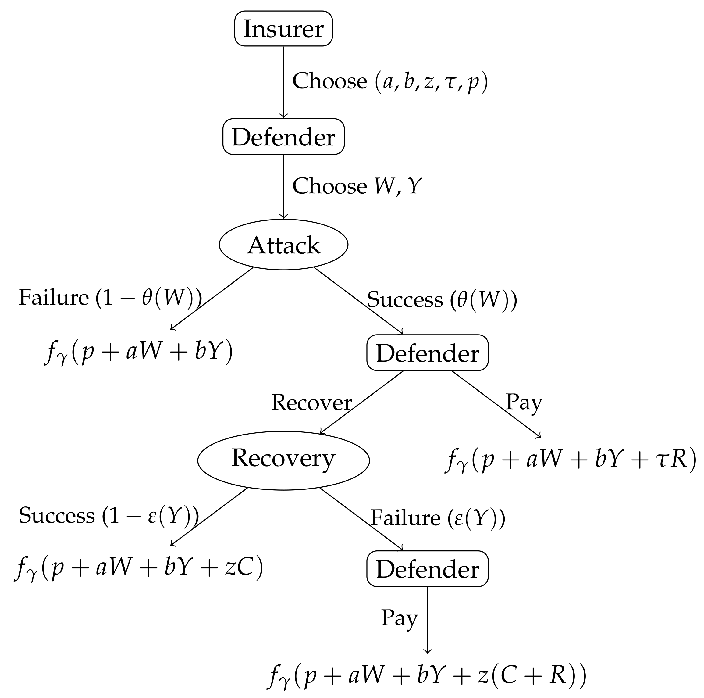
4. The Defender-Insurer (D-I) Game: Model, Analysis, and Results

Now consider the contract between the defender and an insurer providing ransomware insurance. Strictly speaking, this is a two-stage game (more commonly known as a Stackelberg game with a leader and a follower [30]), where the insurer (the leader) sets the format of the contract (what and how contract parameters are to be determined depending on the defender’s actions) and the defender best responds, which then determine the contract terms. This is formulated as a complete information game between the two, thus eliminating typical issues caused by information asymmetry (unobservable actions can worsen moral hazard, and unobservable types lead to adverse selection). This simplification is a first step toward understanding the role insurance plays in the specific case of ransomware attacks; the basic model can then be extended to include the more general issue of information asymmetry.

As mentioned earlier, in the D-I game we shall model the attacker as a non-strategic third party, whose likelihood of success and subsequent ransom demand are input to the D-I model. In doing so we treat the ransomware attack as a constant existence, which is in accordance with the fact that many such attacks are non-targeted with a generic ransom amount set based on empirical and market knowledge rather than on individual victims’ specific information; such an attacker is also effectively agnostic of whether a given victim has ransomware insurance. We will also use the A-D game to obtain the defender’s option outside the insurance contract: $u^o=\mathbb{E}\left[U_d^{*}\right]$ denotes the defender’s equilibrium expected utility outside the contract.

Similar to the A-D game, the defender has two actions prior to an attack: deterrence (W) and backup (Y); and two actions post a successful attack with probability $\theta \left(W\right)$: try to recover data (and possibly pay if recovery fails with probability $\epsilon \left(Y\right)$) and pay immediately.

We will again assume an exponential form for the defender’s utility function, i.e., $U_d=f_{\gamma }\left(x\right)=-e^{\gamma x}$, where x is the total sum cost borne by the defender, including effort, insurance, backup, recovery, ransom payment, and data loss, less coverage. What subset of these appears in the total cost depends on the scenario; these possibilities are shown in Figure 2 in the many different $f_r\left(\right)$ expressions and analyzed below.

To capture all of the above, we will assume a linear insurance contract that consists of the tuple $(0\le p,0<a,b\le 1,0\le z,\tau \le 1)$ and detailed below:

• $p\ge 0$ is the premium the defender pays the insurer for the contact.
• a and b characterize the defender’s fraction of efforts after the insurer subsidies for $W,Y$, respectively; in other words, the actual cost of the effort of the defender are $aW$ and $bY$ with the insurer returning $(1-a)W$ and $(1-b)Y$ to the defender as discounts on the premium. Note that neither a nor b can be 0 (i.e., the insurer cannot subsidize 100% of the effort), for otherwise the defender will seek infinite $W,Y$, respectively. Accordingly, we will define small $\underline{a}$ and $\underline{b}$ that bound a and b away from 0, respectively.
• Upon a successful attack, if the defender decides to recover data first, then the insurer will cover $1-z$ fraction of the total loss; this loss consists of the defender’s recovery cost if recovery is successful, or the recovery cost plus the ransom if recovery fails.
• If the defender decides to pay immediately, then the insurer covers $1-\tau$ fraction of the ransom.

As can be seen, we are affording the insurer multiple options and significant flexibility in designing the insurance contract; this is intended to help us understand questions such as whether the insurer would incentivize deterrence and backup efforts differently, or whether it is in the insurer’s interest to incentivize recovery and discourage immediate payment by offering a low z, and so on. The defender’s utilities under all possible actions and outcomes in this D-I game are illustrated in Figure 2.

Define $U_d^{in}$ to be the defender’s utility inside a cyber insurance contract. Then the expected utility $\mathbb{E}\left[U_d^{in}\right]$ can be written as

$$\mathbb{E}\left[U_d^{in}\right]=\left(1-\theta \left(W\right)+\theta \left(W\right)min\left\{(1-\epsilon \left(Y\right))e^{\gamma zC}+\epsilon \left(Y\right)e^{\gamma z(C+R)},e^{\gamma \tau R}\right\}\right)e^{\gamma (p+aW+bY)}.$$

Define U to be the insurer’s utility. Consider the indicator $\mathbf{F}={\mathbb{1}}_{\left\{(1-\epsilon \left(Y\right))e^{\gamma zC}+\epsilon \left(Y\right)e^{\gamma z(C+R)}\ge e^{\gamma \tau R}\right\}}$, with $\mathbf{F}=1$ indicating that the defender will choose to pay immediately ($A_1=\mathtt{Pay}$) and 0 otherwise ($A_1=\mathtt{Recover}$). Then the insurer’s expected utility is affected by the premium, the effort subsidies, as well as the loss, and can be written as

$$\mathbb{E}\left[U\right]=p-(1-a)W-(1-b)Y-\mathbf{F}·\theta \left(W\right)(1-z)(C+\epsilon (Y\left)R\right)-(1-\mathbf{F})·\theta \left(W\right)(1-\tau )R.$$

4.1. Subgame Perfect Equilibrium

As mentioned earlier, the D-I game is also a sequential-move game that involves two stages. Below we detail the backward induction process we use to find a subgame perfect equilibrium. Denote by $(p^{*},a^{*},b^{*},z^{*},{\tau }^{*})$ the insurer’s equilibrium strategy, and $(W^{*},Y^{*})$ the defender’s. Formally, the subgame perfect equilibrium is the solution to the following optimization problem.

$$\begin{array}{ccc}\hfill \underset{W,Y,p,a,b,z,\tau }{arg\; max}& & p-(1-a)W-(1-b)Y-\mathbf{F}\theta \left(W\right)(1-z)(C+\epsilon (Y\left)R\right)-(1-\mathbf{F})\theta \left(W\right)(1-\tau )R\hfill \end{array}$$

$$\begin{array}{ccc}\hfill s.t.& & \mathbb{E}\left[U^{in}\right]\ge u^o,\hfill \end{array}$$

(6)

$$\begin{array}{ccc}& & W,Y\in \underset{W,Y\ge 0}{arg\; max}\mathbb{E}\left[U^{in}\right],\hfill \\ & & p\ge 0,\underline{a}\le a\le 1,\underline{b}\le b\le 1,0\le z,\tau \le 1.\hfill \end{array}$$

(7)

Recall $u^o=\mathbb{E}\left[U_d^{*}\right]$ is the equilibrium expected utility of the defender outside the contract, i.e., from the previous A-D game presented in Section 3. Here the first constraint (6) ensures individual rationality, i.e., the defender will only enter into the contract if it does not lower their expected utility. The second constraint (7) ensures incentive compatibility, i.e., given the contract terms the defender is going to take actions $W,Y$ to maximize self-interest. It’s not hard to verify the above problem is always feasible.

Lemma 2. 

At the equilibrium, $p^{*}$ can be expressed as

$$p^{*}=\frac{1}{\gamma }log\frac{-u^o}{\left(1-\theta \left(W^{*}\right)+\theta \left(W^{*}\right)min\left\{(1-\epsilon \left(Y^{*}\right))e^{\gamma z^{*}C}+\epsilon \left(Y^{*}\right)e^{\gamma z^{*}(C+R)},e^{\gamma {\tau }^{*}R}\right\}\right)e^{\gamma (a^{*}{W}^{*}+b^{*}{Y}^{*})}}.$$

This is easy to see because at the equilibrium the defender must be indifferent between purchasing and not purchasing the contract (otherwise the insurer can always adjust the premium by the right amount so that equality $\mathbb{E}\left[U_d^{in}\right]=u^o$ is attained while increasing the insurer’s utility). Therefore, $p^{*}$ can be computed by setting equality in Equation (6), yielding the expression above.

In the first stage of this two-stage D-I game, the insurer solves the following two sub-problems that correspond to the defender’s possible actions (pay or recover) in the event an attack is successful.

(a) 

$A_1=\mathtt{Pay}$. The following optimization problem yields equilibrium actions by both the defender and the insurer, denoted by $(W_1,Y_1,a_1,b_1,z_1,{\tau }_1)$, if the defender chooses to pay immediately:

$$\begin{array}{ccc}\hfill \underset{W,Y,a,b,z,\tau }{arg\; max}& & \frac{1}{\gamma }log\left(\frac{-u^o}{1-\theta \left(W\right)+\theta \left(W\right)e^{\gamma \tau R}}\right)-W-Y-\theta \left(W\right)(1-\tau )R\hfill \\ \hfill s.t.& & W,Y\in \underset{W,Y\ge 0}{arg\; min}\left\{\left(1-\theta \left(W\right)+\theta \left(W\right)e^{\gamma \tau R}\right)e^{\gamma (aW+bY)}\right\},\hfill \\ & & (1-\epsilon \left(Y\right))e^{\gamma zC}+\epsilon \left(Y\right)e^{\gamma z(C+R)}\ge e^{\gamma \tau R},\hfill \\ & & \underline{a}\le a\le 1,\underline{b}\le b\le 1,0\le z,\tau \le 1.\hfill \end{array}$$

(8)

(b) 

$A_1=\mathtt{Recover}$. The following optimization problem yields equilibrium actions by both the defender and the insurer, denoted by $(W_2,Y_2,a_2,b_2,z_2,{\tau }_2)$, if the defender chooses to recover data first:

$$\begin{array}{ccc}\hfill \underset{W,Y,a,b,z,\tau }{arg\; max}& & \frac{1}{\gamma }log\left(\frac{-u^o}{1-\theta \left(W\right)+\theta \left(W\right)(1-\epsilon \left(Y\right))e^{\gamma zC}+\theta \left(W\right)\epsilon \left(Y\right)e^{\gamma z(C+R)}}\right)\hfill \\ & & -W-Y-\theta (1-z)(C+\epsilon (Y\left)R\right)\hfill \\ \hfill s.t.& & W,Y\in \underset{W,Y\ge 0}{arg\; min}\left\{\left(1-\theta \left(W\right)+\theta \left(W\right)(1-\epsilon \left(Y\right))e^{\gamma zC}+\theta \left(W\right)\epsilon \left(Y\right)e^{\gamma z(C+R)}\right)e^{\gamma (aW+bY)}\right\},\hfill \\ & & (1-\epsilon \left(Y\right))e^{\gamma zC}+\epsilon \left(Y\right)e^{\gamma z(C+R)}<e^{\gamma \tau R},\hfill \\ & & \underline{a}\le a\le 1,\underline{b}\le b\le 1,0\le z,\tau \le 1.\hfill \end{array}$$

(9)

Lemma 3. 

Both Problem (8) and Problem (9) always have feasible solutions.

Proof. 

Consider Problem (8), take $\tau =0$, $z=1$, $a=1$, $b=1$. We can verify the second constraint holds:

$$\begin{array}{cc}\hfill & (1-\epsilon \left(Y\right))e^{\gamma zC}+\epsilon \left(Y\right)e^{\gamma z(C+R)}=(1-\epsilon \left(Y\right))e^{\gamma C}+\epsilon \left(Y\right)e^{\gamma (C+R)}\hfill \\ \hfill \ge & (1-\epsilon \left(Y\right))e^{\gamma C}+\epsilon \left(Y\right)e^{\gamma C}=e^{\gamma C}\ge 1=e^{\gamma \tau R}.\hfill \end{array}$$

Obtain $(W,Y)$ from the first constraint, and we find a feasible solution $(W,Y,a,b,z,\tau )$. Similarly, for Problem (9), we take $z=0$, $\tau =1$, $a=1$, $b=1$, and derive $(W,Y)$ from the first constraint. It can be easily verified that this $(W,Y,a,b,z,\tau )$ is a feasible solution. □

The way the insurer solves their optimization problem is to compare the solutions to the above two sub-problems, $\mathbb{E}\left[U(p_1,W_1,Y_1,a_1,b_1,z_1,{\tau }_1)\right]$ and $\mathbb{E}\left[U(p_2,W_2,Y_2,a_2,b_2,z_2,{\tau }_2)\right]$; whichever yields higher utility value is the course of action (i.e., pay vs. recover) that the insurer wants to induce the defender to take in the event of an attack. This decision then dictates the optimal contract $(p^{*},a^{*},b^{*},z^{*},{\tau }^{*})$. This is then presented to the defender. Since these contract terms are jointly optimal with the defender’s actions $W^{*},Y^{*}$ with respect to the defender’s utility $U_d^{in}$, the defender best responds with the intended $W^{*},Y^{*}$ for the intended choice (pay vs. recover). This is how the subgame equilibrium is arrived at.

While existence is clear, we have not established the uniqueness of the equilibrium. To compute the equilibrium unambiguously, we will assume the following tie-breaking rules without loss of generality: In the event the two sub-problems yield the same utility for the insurer, they will choose $(p^{*},a^{*},b^{*},z^{*},{\tau }^{*})=(p_1,a_1,b_1,z_1,{\tau }_1)$, resulting in $A_1^{*}=\mathtt{Pay}$ and $W^{*}=W_1,Y^{*}=Y_1$. Note that the two sub-problems cannot yield identical tuples as optimal solutions; this is because the second constraints in the two are mutually exclusive under the same Y. In addition, if two or more contract parameter tuples yield the same utility in the same sub-problem, the insurer breaks the tie by choosing the one with the highest parameter value in the order $(a,b,z,\tau ,p)$, i.e., selecting the one(s) with the highest a, and of those still tied, selecting the one(s) with the highest b, and so on.

4.2. Main Results

While we don’t have closed-form solutions to the above problem, below are a few results that provide some partial characterizations of the equilibrium solution. These properties prove very helpful in our numerical experiments presented in Section 5 as they drastically simplify the solution space. Here we assume an exponential form of $\theta \left(W\right)={\theta }_o{e}^{-\lambda W}$ and $\epsilon \left(Y\right)={\epsilon }_o{e}^{-\mu Y}$.

Proposition 1. 

For the sub-problem in Equation (8), the optimal efforts $(W_1,Y_1)$ is given by

$$Y_1=0,W_1=\left\{\begin{array}{cc}0\hfill & a_1\ge \frac{\lambda (e^{\gamma {\tau }_{1}R}-1){\theta }_o}{\gamma (1+(e^{\gamma {\tau }_{1}R}-1){\theta }_o)}\hfill \\ \frac{1}{\lambda }log\frac{(\lambda -\gamma a_1)(e^{\gamma {\tau }_{1}R}-1){\theta }_o}{\gamma a_1}\hfill & \mathrm{otherwise}\hfill \end{array}\right..$$

Further, for the special case ${\theta }_o=1$ (always being successfully attacked if doing nothing in deterrence), and $R=I$ (ransom demand is at its maximum), then $a_1<\frac{\lambda (e^{\gamma {\tau }_{1}R}-1){\theta }_o}{\gamma (1+(e^{\gamma {\tau }_{1}R}-1){\theta }_o)}$, meaning $W_1=\frac{1}{\lambda }log\frac{(\lambda -\gamma a_1)(e^{\gamma {\tau }_{1}R}-1){\theta }_o}{\gamma a_1}$, i.e., the deterrence effort is strictly positive.

Proof. 

For the first sub-problem, in inspecting the constraints we see W and Y can be optimized separately. The only constraint on Y is $Y\ge 0$, thus the optimal value is 0. The constraint then becomes $W\in arg\; min\left\{(1-\theta )e^{\gamma aW}+\theta e^{\gamma (aW+\tau R)}\right\}$. Solving it gives us the expression given in the theorem.

If $R=I$, we show that $W_1=0,Y_1=0$ will result in the insurer’s utility $\mathbb{E}\left[U_1\right]\le 0$.

First, we show that at the equilibrium of the A-D game, $u^o$ is lower bounded by $-(1-{\theta }_o+{\theta }_o{e}^{\gamma I})$. Consider the case where $W=Y=0$ and $A_1=\mathtt{Pay}$. Then the defender’s expected utility is $\mathbb{E}\left[U_d\right]=-(1-{\theta }_o+{\theta }_o{e}^{\gamma R})\ge -(1-{\theta }_o+{\theta }_o{e}^{\gamma I})$. Therefore at the equilibrium, $u^o\ge -(1-{\theta }_o+{\theta }_o{e}^{\gamma I})$ must hold, otherwise the defender can move to $W=Y=0$, and $A_1=\mathtt{Pay}$ to achieve a higher utility (note that the defender moves first in the game).

Return to the D-I game, with $W_1,Y_1=0$ we have

$$\begin{array}{cc}\hfill \mathbb{E}\left[U_1\right]& =\frac{1}{\gamma }log\frac{-u^o}{1-{\theta }_o+{\theta }_o{e}^{\gamma \tau R}}-{\theta }_o(1-\tau )R\hfill \\ \hfill & \le \frac{1}{\gamma }log\left(\frac{-u^o}{e^{{\theta }_o\gamma \tau R}}\right)-{\theta }_o(1-\tau )R\hfill \\ \hfill & \le \frac{1}{\gamma }log(1-{\theta }_o+{\theta }_o{e}^{\gamma I})-{\theta }_{o}I\hfill \end{array}$$

When ${\theta }_o=1$ the upper bound is non-positive. Thus to ensure there’s a market, we must have $W_1=\frac{1}{\lambda }log\frac{(\lambda -\gamma a_1)(e^{\gamma {\tau }_{1}R}-1){\theta }_o}{\gamma a_1}$. □

Proposition 2. 

For the sub-problem in Equation (9), the optimal efforts $(W_2,Y_2)$ can be characterized as follows depending on the values of $a_2$ and $b_2$:

• If $a_2\ge \frac{\lambda }{\gamma },b_2\ge \frac{\mu }{\gamma }$, then $W_2=Y_2=0$;
• If $a_2\ge \frac{\lambda }{\gamma },b_2<\frac{\mu }{\gamma }$, then $W_2=0$, and

  $$Y_2=\left\{\begin{array}{cc}0\hfill & b_2\ge \frac{\mu }{\gamma }\frac{1}{1+\frac{1-{\theta }_o+{\theta }_o{e}^{\gamma z_{2}C}}{{\theta }_o{\epsilon }_o{e}^{\gamma z_{2}C}(e^{\gamma z_{2}R}-1)}}\hfill \\ \frac{1}{\mu }log\frac{{\theta }_o{\epsilon }_o(e^{\gamma z_2(C+R)}-e^{\gamma z_{2}C})(\mu -\gamma b_2)}{\gamma b_2(1-{\theta }_o+{\theta }_o{e}^{\gamma z_{2}C})}\hfill & \mathrm{otherwise}\hfill \end{array}\right.;$$
• If $a_2<\frac{\lambda }{\gamma },b_2\ge \frac{\mu }{\gamma }$, then $Y_2=0$, and

  $$W_2=\left\{\begin{array}{cc}0\hfill & a_2\ge \frac{\lambda }{\gamma }\left(1-\frac{1}{1+{\theta }_o({\epsilon }_o{e}^{\gamma z_2(C+R)}+(1-{\epsilon }_o)e^{\gamma z_{2}C}-1)}\right)\hfill \\ \frac{1}{\lambda }log\frac{(\lambda -\gamma a_2){\theta }_o}{\gamma a_2}\left({\epsilon }_o{e}^{\gamma z_2(C+R)}+(1-{\epsilon }_o)e^{\gamma z_{2}C}-1\right)\hfill & \mathrm{otherwise}\hfill \end{array}\right.;$$
• If $a_2<\frac{\lambda }{\gamma },b_2<\frac{\mu }{\gamma }$, then

  $$W_2,Y_2\in \underset{W\ge 0,Y\ge 0}{arg\; min}\left\{e^{\gamma aW+\gamma bY}+{\theta }_o(e^{\gamma zC}-1)e^{(\gamma a-\lambda )W+\gamma bY}+{\theta }_o{\epsilon }_o{e}^{\gamma zC}(e^{\gamma zR}-1)e^{(\gamma a-\lambda )W+(\gamma b-\mu )Y}\right\}.$$

Proof. 

The expected utility of the defender in this case can be simplified.

$$\mathbb{E}\left[U_d^{in}\right]=e^{\gamma (aW+bY)}+{\theta }_o(e^{\gamma zC}-1)e^{(\gamma a-\lambda )W+\gamma bY}+{\theta }_o{\epsilon }_o{e}^{\gamma zC}(e^{\gamma zR}-1)e^{(\gamma a-\lambda )W+(\gamma b-\mu )Y}.$$

It’s not hard to verify that when $\gamma a\ge \lambda$, then $W_2=0$, since the first term is strictly increasing while the last two are non-decreasing with W. Similarly, $\gamma b\ge \mu$ will ensure $Y_2=0$. When $W_2=0$, the optimal $Y_2={arg\; min}_{Y\ge 0}\{e^{\gamma bY}+{\theta }_o(e^{\gamma zC}-1)e^{\gamma bY}+{\theta }_o{\epsilon }_o{e}^{\gamma zC}(e^{\gamma zR}-1)e^{(\gamma b-\mu )Y}\}$. Solving it yields the closed form of $Y_2$. Similarly, when $Y_2=0$, we can also get a closed form for $W_2$. □

Note that, in the last case of Proposition 2, the closed form of $(W_2,Y_2)$ is not presented, however using KKT conditions [31] we can numerically solve the problem efficiently.

Finally, we can also bound the insurer’s maximum possible utility.

Proposition 3. 

At the equilibrium, the expected utility of the insurer is upper bounded by $\frac{1}{\gamma }log(-u^o)$.

Proof. 

$$\begin{array}{cc}\hfill \mathbb{E}\left[U\right]& =p-(1-a)W-(1-b)Y-\mathbf{F}·\theta \left(W\right)(1-z)(C+\epsilon (Y\left)R\right)-(1-\mathbf{F})·\theta \left(W\right)(1-\tau )R\hfill \\ \hfill & \le p\le \frac{1}{\gamma }log(-u^o),\hfill \end{array}$$

where the last two inequalities come from Lemma 2. □

5. Numerical Evaluation

To further analyze the A-D and D-I games, in this section we will examine and visualize the equilibria of these games using numerical simulations. We will assume an exponential form for $\theta \left(W\right)$ and $\epsilon \left(Y\right)$, i.e., $\theta \left(W\right)={\theta }_o{e}^{-\lambda W}$ and $\epsilon \left(Y\right)={\epsilon }_o{e}^{-\mu Y}$. We also set $I=1$ for our experiments, therefore computed costs/rewards in this section are all relative to the data value. No external data is used in the experiment. All the data are generated on-the-fly in the associated scripts. We perform all the experiments using Matlab [32] on a single PC.

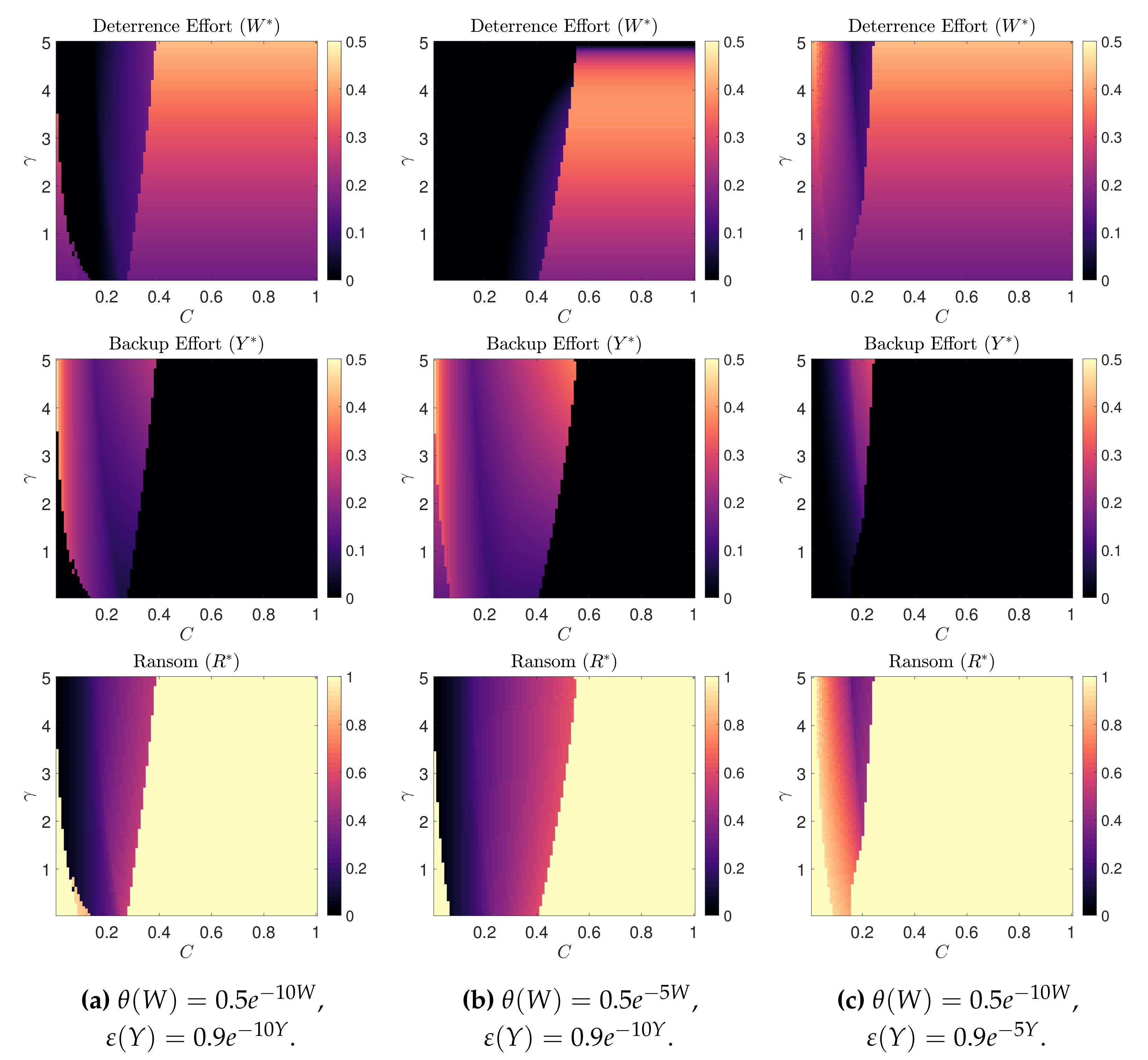
5.1. A-D Model

To visualize how the equilibrium strategies of the attacker and the defender change with respect to the recovery cost C and risk attitude $\gamma$, we compute and plot $W^{*}$, $Y^{*}$, and $R^{*}$ as a function of these parameters. Figure 3 displays our results, where we have generated plots using different $\theta \left(W\right)$ and $\epsilon \left(Y\right)$.

As discussed in Section 3, we can divide the game parameters into three regions depending on the equilibrium strategy types they support. On the left side of each figure (low C) the attacker chooses $R^{*}=I$, while the defender will attempt recovery before paying the ransom. On the right side of each figure (high C) the attacker will again choose $R^{*}=I$, while the defender will pay the ransom immediately. In the region between these two, the attacker will lower the ransom to ensure that the defender will pay without attempting recovery. While both $\gamma$ and C play a role in determining the type of equilibrium, we observe that C is the main driver. An increasing C forces the defender to shift from attempting recovery to paying ransom immediately. Note that Laszka et al. [9] derive a similar result with respect to the unit cost of backup in their model.

In the high recovery cost region, the backup effort is abandoned as discussed in Section 3, and the defender has to rely on deterrence effort to lower the expected loss. Interestingly, however, in the other two regions, the attacker seems to favor one type of defense over the other, with one of $W^{*}$ or $Y^{*}$ being low. We also observe that a more effective backup effort relative to the deterrence effort (the second column in Figure 3) seems to expand the middle region.

Another interesting observation is that, in the middle region, though the defender pays ransom immediately (backup is not used), the backup effort is still made (and is significantly higher than the deterrence effort in the first and the second columns). As mentioned earlier, in this case, backup is used as a credible threat to the attacker to lower the ransom. It is indeed noteworthy that the highest backup effort occurs in this region: when the defender has invested the most in backup, they will also choose to pay immediately. This observation is supported by Theorem 1, where ${\epsilon }^{*}<{\epsilon }_l$ is followed by accepting a lower ransom.

Though C is the main driver, a larger $\gamma$ enlarges the width of the middle region, meaning that a more risk-averse defender is more willing to accept the attacker’s low ransom compromise. A large $\gamma$ also shrinks (and in some cases completely eliminates) the recovery region.

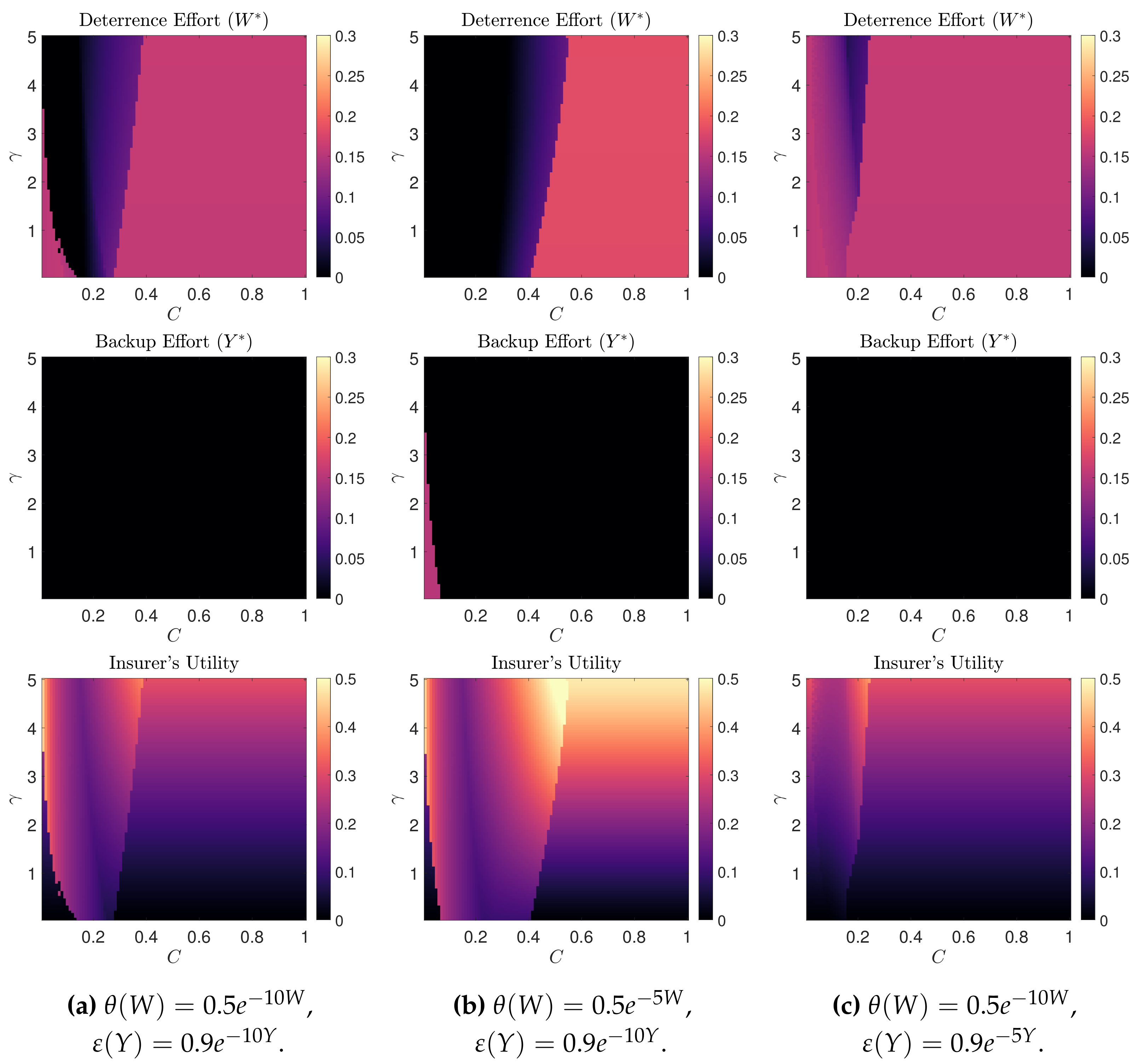
5.2. D-I Model

We also visualize the equilibrium of the D-I game in Figure 4, using the same parameters as Figure 3. We shall assume that the attacker acts according to the equilibrium of the A-D game, i.e., the ransom amount at each point is equal to what is presented in Figure 3.

Comparing the two games, we observe that the recovery region remains roughly the same, which means the defender basically keeps the original decision making regardless of the contract. However, the defender’s efforts are very different. The defender will almost always abandon the backup effort under insurance, while the deterrence effort is reduced but positive as compared to the equilibrium of the A-D game. While the presence of moral hazard is not surprising, it is interesting to see that it affects the backup effort more drastically than the deterrence effort. An explanation for this is that the deterrence effort controls the overall probability of a successful attack, while the backup effort only affects the expected loss when going down the recovery path. Therefore, the latter has a smaller effect on the overall loss, and is abandoned first in the presence of insurance; this is compounded by the fact that the attacker is non-strategic in the D-I game, a consequence of which is that the backup effort cannot be used as a credible threat, unlike in the A-D game.

On the insurer’s utility, we first observe that it is positive in almost all cases. In particular, for large $\gamma$, it is nearly half of the data value in some cases, clearly demonstrating the existence of such a market for insurance. Note that the optimal $a^{*},b^{*}$ are at the minimum values $\underline{a}$ and $\underline{b}$, respectively, with ${\tau }^{*}=0$ for the pay region, and $z^{*}=0$ for the recovery region. These values suggest that the defender essentially only pays the premium, while the costs of effort and losses from a successful attack are all but completely covered by the insurer.

In addition, with the introduction of insurance, the attacker gains a slightly higher payout due to the reduction of the defender’s effort. Note that the defender’s utility remains the same inside and outside of the contract. This means that the attacker is essentially cutting into the insurer’s potential profit. Nevertheless, the insurer is still making a profit by taking advantage of the defender’s risk-aversion, with their profit increasing as the defender becomes more risk-averse.

6. Limitations and Discussion

One obvious limitation of the current study is the fact that the ransomware ecosystem is modeled as a two separate, albeit connected, two-player games. A more accurate and comprehensive treatment of the subject might require a three-way A-D-I game model, where the attacker is also strategic. This remains an interesting direction of future work.

Other possible extensions of the work include analyzing and providing potential solutions for the moral hazard issue and studying the problem under incomplete information assumptions.

It is worth noting that different parties in this ransomware ecosystem typically have different risk perceptions. In particular, an insurer faces not just one customer (defender) but many, and the risk pooling effect justifies less risk-aversion (in theory that is, not necessarily in practice). For this reason, in our models, the defender is risk-averse – its utility is a concave (decreasing) function of the total cost – but the insurer is risk neutral – its utility is a linear function, the simple sum of the total profit (or equivalently, total cost). This is not the same as studying a population game with multiple defenders each having their own policy, but takes into account the difference in the insurer’s risk perception.

7. Conclusions

This paper presented and analyzed two game theoretic models involving ransomware attacks.

In the Attacker-Defender (A-D) game we analyze the strategic interaction between an attacker (whose action is choosing a ransom amount) and a defender deciding on their effort levels. We identify three types of equilibria, mainly dependent on the cost of data recovery and the level of risk-aversion for the defender. Our findings show that the backup effort is often used as a credible threat against the attacker to induce a lower ransom, rather than as a real recovery measure. We also detect that a highly risk-averse defender is more likely to arrive at a compromise with the attacker, accepting a lower ransom and paying immediately.

Our analysis of the Defender-Insure (D-I) game suggests that the introduction of insurance causes the defender to almost completely abandon the backup effort and reduce their deterrence effort. At the same time, the insurer offers to cover all efforts through premium discounts and cover all potential losses. The insurer’s profit is then derived from the risk-aversion of the defender, which increases as the defender becomes more risk-averse. However, in presence of insurance, the attacker also enjoys a higher payout due to lower efforts by the defender. Nevertheless, our empirical results show that there is still a market for insurance.