Article

Robust Satisfaction of Metric Interval Temporal Logic Objectives in Adversarial Environments

1
Network Security Lab, Department of Electrical and Computer Engineering, University of Washington, Seattle, WA 98195, USA
2
Electrical and Computer Engineering, Western Washington University, Bellingham, WA 98225, USA
3
Department of Electrical and Systems Engineering, Washington University in St. Louis, St. Louis, MO 63130, USA
*
Author to whom correspondence should be addressed.
Games 2023, 14(2), 30; https://doi.org/10.3390/g14020030
Submission received: 31 January 2023 / Revised: 22 March 2023 / Accepted: 22 March 2023 / Published: 30 March 2023
(This article belongs to the Special Issue Game-Theoretic Analysis of Network Security and Privacy)

Abstract

:
This paper studies the synthesis of controllers for cyber-physical systems (CPSs) that are required to carry out complex time-sensitive tasks in the presence of an adversary. The time-sensitive task is specified as a formula in the metric interval temporal logic (MITL). CPSs that operate in adversarial environments have typically been abstracted as stochastic games (SGs); however, because traditional SG models do not incorporate a notion of time, they cannot be used in a setting where the objective is time-sensitive. To address this, we introduce durational stochastic games (DSGs). DSGs generalize SGs to incorporate a notion of time and model the adversary’s abilities to tamper with the control input (actuator attack) and manipulate the timing information that is perceived by the CPS (timing attack). We define notions of spatial, temporal, and spatio-temporal robustness to quantify the amounts by which system trajectories under the synthesized policy can be perturbed in space and time without affecting satisfaction of the MITL objective. In the case of an actuator attack, we design computational procedures to synthesize controllers that will satisfy the MITL task along with a guarantee of its robustness. In the presence of a timing attack, we relax the robustness constraint to develop a value iteration-based procedure to compute the CPS policy as a finite-state controller to maximize the probability of satisfying the MITL task. A numerical evaluation of our approach is presented on a signalized traffic network to illustrate our results.

1. Introduction

Cyber-physical systems (CPSs) are playing increasingly important roles in multiple applications, including autonomous vehicles, robotics, and advanced manufacturing [1]. In many of these applications, the CPS is expected to satisfy complex, time-critical objectives in dynamic environments with autonomy. An example is a scenario where a drone has to periodically surveil a target region in its environment. One way to specify requirements on the CPS behavior is through a temporal logic framework [2] such as metric interval temporal logic (MITL) or signal temporal logic (STL). The verification of satisfaction of the temporal logic objective can then be achieved by applying principles from model checking [2,3] to a finite transition system that abstracts the CPS [4,5,6,7]. Solution techniques to verify such an objective usually return a ‘yes/no’ output, which indicates if the behavior of the CPS will satisfy the desired task and if it is possible to synthesize a control policy to satisfy this objective.
However, such binary-valued verification results may not be adequate when an adversary can inject inputs that affect the behavior of the CPS. Small perturbations can result in significantly large changes in the output of a CPS and can lead to violations of the desired task. The authors of [8,9] defined a notion of robustness degree to quantify the extent to which a CPS could tolerate deviations from its nominal behavior without resulting in violation of the desired specification.
For time-critical CPSs, an adversary could launch attacks on clocks of the system (by timing attack) and the inputs to the system (by actuator attack). In the latter case, stochastic games (SGs) have been used to model the interaction between the CPS and the adversary [10]. However, SGs do not include information about the time taken for a transition between two states. To bridge this gap, we introduce durational stochastic games (DSGs). In addition to transition probabilities between states under given actions of the CPS and adversary, a DSG encodes the time taken for the transition as a probability mass function. Although DSGs present a modeling formalism for time-critical objectives, they introduce an additional attack surface that can be exploited by an adversary.
In this paper, we synthesize controllers to satisfy an MITL specification that can be represented by a deterministic timed Büchi automaton with a desired robustness guarantee. The robustness guarantee quantifies how sensitive the synthesized policy (that satisfies the MITL task) will be to disturbances and adversarial inputs. The adversary is assumed to have the following abilities: it can tamper with the input to the defender through an actuator attack [11], and it can affect the time index observed by the CPS by effecting a timing attack [12]. An actuator attack could steer the DSG away from a target set of states, while a timing attack will prevent it from satisfying the objective within the specified time interval.
To address perturbations originating from different attack surfaces (timing information and system inputs), we develop three notions of robustness, namely spatial, temporal, and spatio-temporal robustness. Spatial robustness is defined over discrete timed words and quantifies the maximum perturbation that can be tolerated by timed words so that the desired tasks can still be satisfied in the absence of timing attacks. The temporal robustness characterizes the maximum timing perturbation that can be tolerated by a CPS such that the given MITL objective will not be violated. We introduce a notion of spatio-temporal robustness that unifies the concepts of spatial and temporal robustness. Using these three notions of robustness, we develop algorithms to estimate them and compute controllers for CPSs to guarantee that the given MITL objective can be satisfied with the desired robustness guarantee. This paper makes the following contributions:
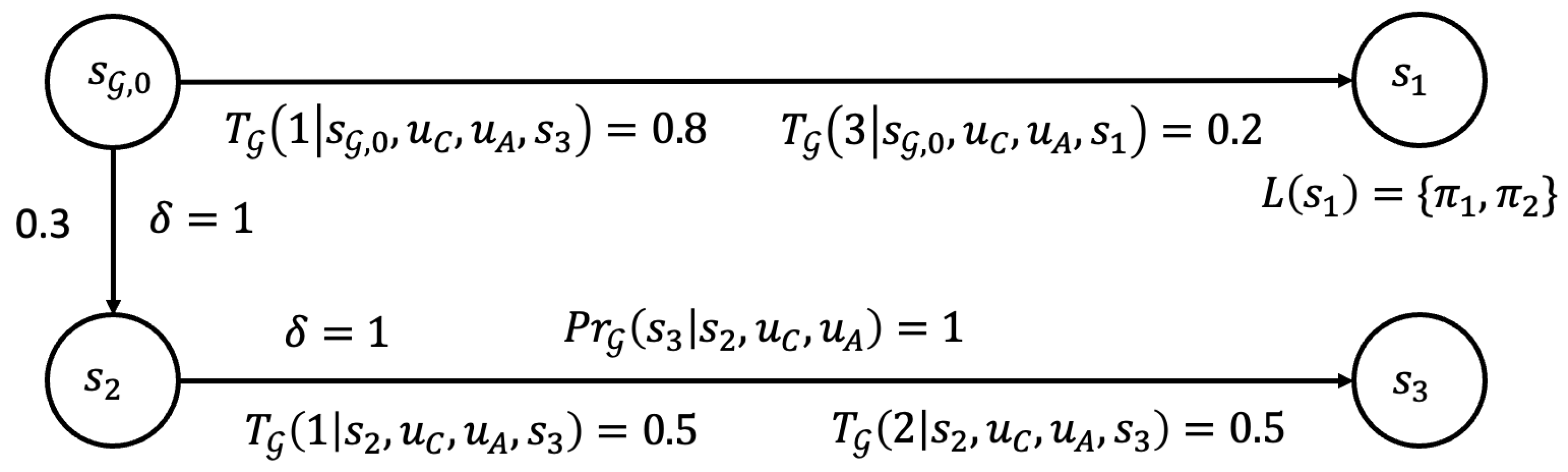
  • We introduce durational stochastic games (DSGs) to model the interaction between the CPS that has to satisfy a time-critical objective and an adversary who can initiate actuator and timing attacks.
  • We define notions of spatial, temporal, and spatio-temporal robustness, which quantify the robustness of system trajectories to spatial, temporal, and spatio-temporal perturbations, respectively, and present computational procedures to estimate them. We design an algorithm to compute a policy for the CPS (defender) with a robustness guarantee when the adversary is limited to effecting only actuator attacks.
  • We demonstrate that the defender cannot correctly estimate the spatio-temporal robustness when the adversary can initiate both actuator and timing attacks. We relax the robustness constraints in such cases and present a value iteration-based procedure to compute the defender’s policy, represented as a finite-state controller, to maximize the probability of satisfying the MITL objective.
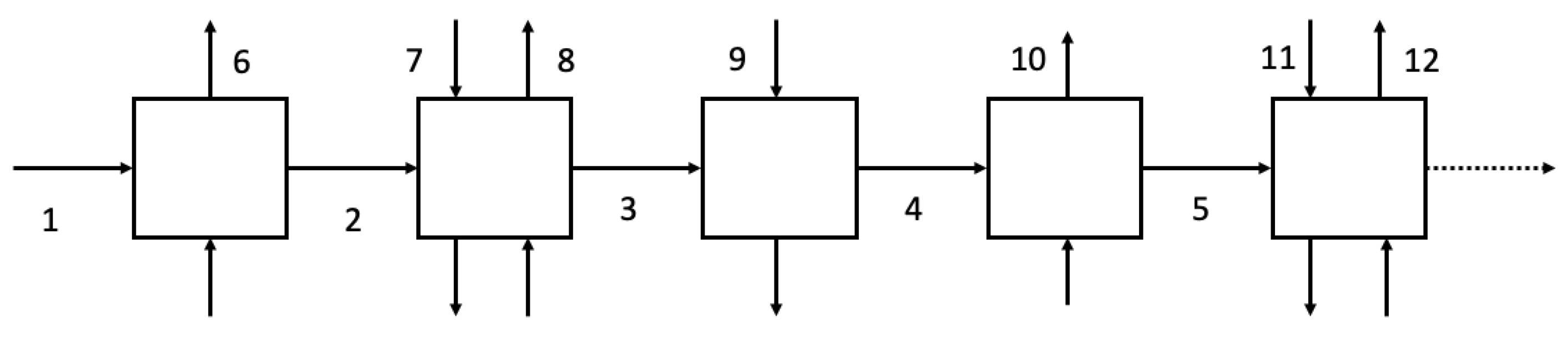
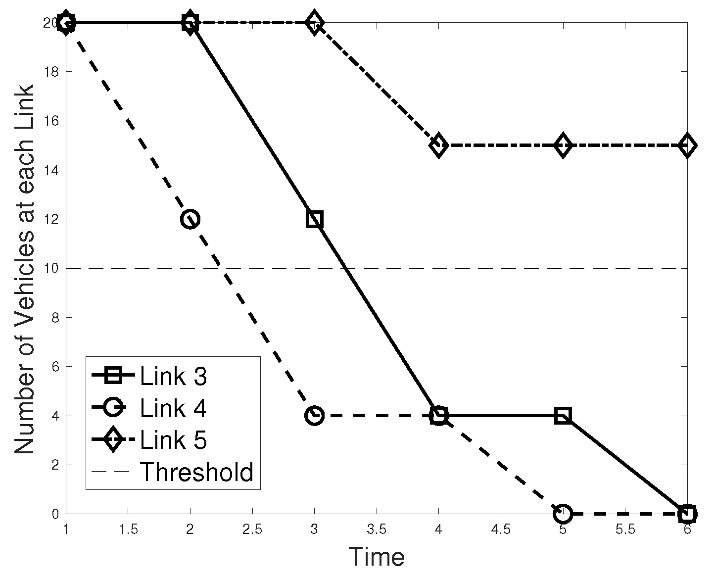
  • We evaluate our approach on a signalized traffic network. We compare our approach with two baselines and show that it outperforms both baselines.
The remainder of this paper is organized as follows. Section 2 discusses related work. Section 3 provides background on MITL and deterministic timed Büchi automata. We define the DSG and notions of robustness in Section 4 and formally state the problem of interest. Section 5 and Section 6 present our results when the adversary is limited to initiating only actuator attacks and when it can effect both actuator and timing attacks, respectively. The experimental results are presented in Section 7. Section 8 concludes the paper.

2. Related Work

For a single agent, semi-Markov decision processes (SMDPs) [13] can be used to model Markovian dynamics, where the time taken for transitions between states is a random variable. SMDPs have been used in production scheduling [14] and the optimization of queues [15].
Stochastic games (SGs) generalize MDPs when there is more than one agent taking an action [16]. SGs have been widely adopted to model strategic interactions between CPSs and adversaries. For example, a zero-sum SG was formulated in  [17] to allocate resources to protect power systems against malicious attacks. Two SGs were developed in [18] to detect intrusions to achieve secret and reliable communications. The satisfaction of complex objectives modeled by linear temporal logic (LTL) formulae for zero-sum two-player SGs was presented in [10], where the authors synthesized controllers to maximize the probability of satisfying the LTL formula. However, this approach will not apply when the system has to satisfy a time-critical specification and the adversary can launch a timing attack.
Timed automata (TA) [3] finitely attach many clock constraints to each state. A transition between any two states will be influenced by the satisfaction of the clock constraints in the respective states. There has been significant work performed in the formulation of timed temporal logic frameworks, a detailed survey of which is presented in [19]. Metric interval temporal logic (MITL) [20] is one such fragment that allows for the specification of formulae that explicitly depend on time. Moreover, an MITL formula can be represented as a TA [20,21] that will have a feasible path in it if and only if the MITL formula is true.
Control synthesis under metric temporal logic constraints was studied for motion planning applications in [6,7,22,23]. The authors of [22] considered a vehicle routing problem to meet MTL specifications by solving a mixed integer linear program. Timed automaton-based control synthesis under a subclass of MITL specifications was studied in [6,7]. Cooperative task planning of a multi-agent system under MITL specifications was studied in [24]. In comparison, we consider the actions of an adversarial player, whose objective is opposite to that of the defender. This leads to a modeling of the interaction between the adversary and defender as an SG. Moreover, the previous works have limited their focus to a certain fragment of the MITL, whereas this paper offers a generalized treatment to arbitrary MITL formulae.
Finite-state controllers (FSCs) were used to simplify the policy iteration procedure for POMDPs in [25]. The satisfaction of an LTL formula of a POMDP was presented in [26]. This was extended to the case with an adversary who also only had partial observation of the environment and whose goal was to prevent the defender from satisfying the LTL formula in [27,28]. These treatments, however, did not account for the presence of timing constraints on the satisfaction of a temporal logic formula.
Control synthesis for control systems under disturbances with robustness guarantees has been extensively studied [29,30,31,32]. Such robustness guarantees can be categorized as a notion of spatial robustness. Robust satisfaction of temporal logic tasks have been studied for signal monitoring and property verification. A notion of robustness degree for continuous signals was defined in [8] by computing a distance between the given timed behavior and the set of behaviors that satisfy a property expressed in temporal logic. Our notion of spatial robustness is defined over discrete timed words using the Levenshtein distance, which distinguishes our approach from [8]. The robustness degree between two LTL formulae was introduced in [33]. The authors of [34] adopted a different approach and used the weighted edit distance to quantify a measure of robustness. The notion of temporal robustness was also investigated in [9]. There are three differences between our definition of temporal robustness and that found in [9]. First, the temporal robustness in [9] is defined for a specific trace. In our framework, as the DSG is not deterministic, there could be multiple traces that satisfy the MITL objective under the defender and adversary policies. Therefore, we define temporal robustness with respect to the policies of the defender and adversary and the MITL specification. Second, the temporal robustness of a real-valued signal is computed as the maximum amount of time units by which we can shift on the rising/falling edge of a ‘characteristic function’ in [9]. In comparison, we work with discrete timed words. Finally, our work considers the presence of an adversary, while [9] assumes a single agent. Robust control under signal temporal logic (STL) formulae has been studied based on notions of space robustness [35,36] and temporal robustness [37,38]. These works did not consider the presence of an adversary.
A preliminary version of this paper [39] synthesized policies to satisfy MITL objectives under actuator and timing attacks without robustness guarantees. In this paper, we define three robustness degrees and develop algorithms to compute these quantities. We show that any defender policy that provides a positive robustness degree is an almost-sure satisfaction policy, which is stronger than the quantitative satisfaction policies synthesized in [39].

3. MITL and Timed Automata

We introduce the syntax and semantics of metric interval temporal logic and its equivalent representation as a timed automaton. We use R ,   R 0 ,   N , and Q 0 to denote the sets of real numbers, non-negative reals, positive integers, and non-negative rationals, respectively. Vectors are represented by bold symbols. The comparison between vectors v 1 and v 2 is element-wise, and v ( i ) denotes the i-th element of v . Given a set of atomic propositions Π , a metric interval temporal logic (MITL) formula is inductively defined as
φ : = | π | ¬ φ | φ 1 φ 2 | φ 1 U I φ 2 ,
where π Π is an atomic proposition and I is a non-singular time interval with integer end-points. MITL admits derived operators such as ‘constrained eventually’ ( I φ :   = U I φ ) and ‘constrained always’ ( I φ : = ¬ ( I ¬ φ ) ). Throughout this paper, we assume that I is bounded. We further rewrite the given MITL formula in the negation normal form so that negations only appear in front of atomic propositions. We augment the atomic proposition set Π so that any atomic proposition π and its negation ¬ π are both included in Π .
We focus on the pointwise MITL semantics [40]. A timed word is an infinite sequence ρ = ( a 0 , t 0 ) ( a 1 , t 1 ) , where a i 2 Π ; t i R 0 is the time index with t i + 1 > t i i 0 . We denote a 0 , a 1 , as a word over Π and t 0 ,   t 1 ,   as a time sequence. With ρ ( i ) = ( a i , t i ) , we define: UNTIME ( ρ ) : = a 0 , a 1 , , and v a l ( ρ ) : = t 0 ,   t 1 , .
We interpret MITL formulae over timed words as follows.
Definition 1 
(MITL Semantics). Given a timed word ρ and an MITL formula φ, the satisfaction of φ at position j, denoted as ( ρ , j ) φ , is inductively defined as follows:
1.
( ρ , j ) if and only if (iff) ( ρ , j ) is true;
2.
( ρ , j ) π iff π a j ;
3.
( ρ , j ) ¬ φ iff ( ρ , j ) does not satisfy φ;
4.
( ρ , j ) φ 1 φ 2 iff ( ρ , j ) φ 1 and ( ρ , j ) φ 2 ;
5.
( ρ , j ) φ 1 U I φ 2 iff k j such that ( ρ , k ) φ 2 , t k t j I and ( ρ , m ) φ 1 holds for all j m < k .
We denote ρ φ if ( ρ , 0 ) φ . The satisfaction of an MITL formula can be equivalently associated with accepting words of a timed Büchi automaton (TBA) [20]. Let C = { c 1 , , c M } be a finite set of clocks. Define a set of clock constraints Φ ( C ) over C as ξ = | | c δ | ξ 1 ξ 2 , where { , , < , > } , c ,   c C are clocks, and δ Q is a non-negative rational number. In this paper, we focus on a subclass of MITL formulae that can be equivalently represented as deterministic timed Büchi automaton, which are defined as follows.
Definition 2 
(Deterministic Timed Büchi Automaton [3]). A deterministic timed Büchi automaton (DTBA) is a tuple A = ( Q , 2 Π , q 0 , C , Φ ( C ) , E , F ) , where Q is a finite set of states, 2 Π is an alphabet over atomic propositions in Π , q 0 is the initial state, E Q × Q × 2 Π × 2 C × Φ ( C ) is the set of transitions, and F Q is the set of accepting states. A transition < q , q , a , C , ϕ > E if A enables the transition from q to q when a subset of atomic propositions a 2 Π and clock constraints ϕ Φ ( C ) evaluate to true. The clocks in C C are reset to zero after the transition.
We present the DTBA representing MITL formula φ = [ 2 , 3 ] π as an example in Figure 1. In this figure, the states Q and transitions E are represented by circles and arrows, respectively. Here, the initial state is q 0 . The set of accepting states is F = { q 2 } . Consider the transition from initial state q 0 to state q 2 . The transition < q 0 , q 2 , π , c , ϕ > can take place if atomic proposition π is evaluated to be true and clock constraint ϕ ( c ) defined on clock c satisfies 2 c 3 . Furthermore, the clock c is reset to zero after the transition.
Given the set of clocks C, v : C V is the valuation of C, where V Q | C | . Let v ( c ) be the valuation of clock c C . We say v = 0 if v ( c ) = 0 for all c C . Given δ R 0 , we let v + δ : = [ v ( 1 ) + δ , , v ( | C | ) + δ ] T . A configuration of A is a pair ( q , v ) , where q Q is a state of A . Suppose a transition < q , q , a , C , ξ > is taken after δ time units. Then, the DTBA is transited from configuration ( q , v ) to ( q , v + δ ) such that v + δ ξ , v ( c ) = v ( c ) + δ for all c C and v ( c ) = 0 for all c C . We denote the transition between these configurations as ( q , v ) a , δ ( q , v + δ ) . A run of A is a sequence of such transitions between configurations β : = ( q 0 , v 0 ) a 0 , δ 0 ( q 1 , v 1 ) . A feasible run β on A is accepting iff it intersects with F infinitely often.

4. Problem Setup and Formulation

In this section, we propose durational stochastic games that generalize stochastic games and present the defender and adversary models in terms of the information available to them. We then define three robustness degrees and state the problem of interest.

4.1. Environment, Defender, and Adversary Models

We introduce durational stochastic games as a generalization of stochastic games [10]. Different from SGs, DSGs model (i) the timing information for transitions between states and (ii) an attack surface resulting from the timing information.
An SG is defined as follows:
Definition 3 
(Stochastic game). A (labeled) stochastic game SG is a tuple SG = ( S , U C , U A , P r , Π , L ) , where S is a finite set of states, U C is a finite set of actions of the defender, U A is a finite set of actions of an adversary, and P r : S × U C × U A × S [ 0 , 1 ] is a transition function where P r ( s , u C , u A , s ) is the probability of a transition from state s to state s when the defender takes action u C and the adversary takes action u A . Π is a set of atomic propositions. L : S 2 Π is a labeling function mapping each state to a subset of propositions in Π .
The SG in Definition 3 cannot be used to verify satisfaction of an MITL objective as it does not include a notion of time. We define durational stochastic games to bridge this gap. DSGs incorporate a notion of time taken for a transition between states and also models the ability of an adversary to modify this timing information.
Definition 4 
(Durational stochastic game). A (labeled) durational stochastic game (DSG) is a tuple G = ( S G , s G , 0 , U C , U A , I n f G , C , I n f G , A , P r G , T G , Π , L , C l ) . S G is a finite set of states, s G , 0 is the initial state, and U C , U A are finite sets of actions. I n f G , C : S G × R 0 ( S G × R 0 ) * and I n f G , A : S G × R 0 ( S G × R 0 × U C ) * are information sets of the defender and adversary, respectively, where ( · ) * is the Kleene operator. P r G : S G × U C × U A × S G [ 0 , 1 ] encodes P r G ( s G | s G , u C , u A ) , the transition probability from state s G to s G when the controller and adversary take actions u C and u A . T G : S G × U C × U A × S G × Δ [ 0 , 1 ] is a probability mass function. T G ( δ | s G , u C , u A , s G ) denotes the probability that a transition from s G to s G under actions u C and u A takes δ Δ time units, where Δ is a finite set of time units that each transition of DSG can possibly take to complete. Π is a set of atomic propositions. L : S G 2 Π is a labeling function that maps each state to atomic propositions in Π that are true in that state, and C l is a finite set of clocks.
The set of admissible actions that can be taken by the defender (adversary) in a state s S G is denoted as U C ( s ) ( U A ( s ) ). A path on G is a sequence of states w : = s 0 δ 0 u C , 0 , u A , 0 s 1 δ i u C , i , u A , i s i + 1 such that s 0 = s G , 0 , P r G ( s i + 1 | s i , u C , i , u A , i ) > 0 and T G ( δ | s i , u C , i , u A , i , s i + 1 ) > 0 for some u C , i U C ( s i ) , u A , i U A ( s i ) , and δ Δ for all i 0 . Consider the DSG with S G = { s G , 0 , s 1 , s 2 , s 3 } , U C = { u C } , and U A = { u A } presented in Figure 2 as an example. We have that w = s 0 1 u C , u A s 2 1 u C , u A s 3 is a finite path. We denote the set of finite (infinite) paths by ( S G × R 0 ) * ( ( S G × R 0 ) ω ). Given a path w, L ( w ) : = L ( s G , 0 ) , L ( s 1 ) , , is the sequence of atomic propositions corresponding to states in w. The sequence of state-time tuples in w is obtained as ( s 0 , k 0 ) ,   ( s 1 , k 1 ) , , where k i + δ i = k i + 1 , i = 0 , 1 , .
For the defender, a deterministic policy  μ : ( S G × R 0 ) * U C is a map from the set of finite paths to its actions. A randomized policy  μ : ( S G × R 0 ) * D ( U C ) maps the set of finite paths to a probability distribution over its actions. A policy is memoryless if it only depends on the the most recent state.
Consider a path w in G . At a state s, the information set of the defender is I n f G , C w ( s , k C ) : = { ( s G , 0 , 0 ) , , ( s , k C ) } , where k C is the time perceived by the defender when it reaches s along w. For example, given the finite path w = s 0 1 u C , u A s 2 1 u C , u A s 3 for the DSG presented in Figure 2, information set I n f G , C w ( s 2 , k C ) = { ( s G , 0 , 0 ) , ( s 1 , 1 ) } . For the adversary, I n f G , A ( s , k A ) : = { ( s G , 0 , 0 ) , , ( s , k A ) } { μ } , where k A is the time observed by the adversary at s, and μ is the defender’s policy. Information sets of the defender and adversary are given by I n f G , C ( s , k C ) : = w I n f G , C w ( s , k C ) and I n f G , A ( s , k A ) : = w I n f G , A w ( s , k A ) .
We assume that the initial time is 0, and this is known to both agents. The adversary having knowledge of the policy μ committed to by the defender introduces an asymmetry between the information sets of the two agents. We note that although the adversary is aware of the defender’s randomized policy, it does not know the exact action u C . This is also known as the Stackelberg setting in game theory. We assume a concurrent Stackelberg setting in that both the defender and adversary take their actions at each state simultaneously.
The solution concept to a Stackelberg game is a Stackelberg equilibrium, which is defined as follows.
Definition 5 
(Stackelberg equilibrium [16]). A tuple ( μ , ( τ , γ ) ) is a Stackelberg equilibrium if μ = arg max μ Q C ( μ , B R ( μ ) ) , where Q C ( μ , ( τ , γ ) ) and Q A ( μ , ( τ , γ ) ) are the expected utilities of the defender and adversary under policies μ and ( τ , γ ) , respectively, and B R ( μ ) = { ( τ , γ ) : ( τ , γ ) = arg max ( τ , γ ) Q A ( μ , ( τ , γ ) ) } .
If B R ( μ ) contains multiple adversary policies, the defender will arbitrarily pick one. During an actuator attack, the adversary can manipulate state transitions in G as its actions u A will influence the transition probabilities P r G . The adversary could also exploit the attack surface that will be introduced as a consequence of including timing information. We term this a timing attack. In this paper, we consider the worst-case scenario and assume that the adversary knows the correct time index at each time k. However, it can manipulate the timing information perceived by the defender through T G . Thus, the time index k C perceived by the defender need not be the same as that known to the adversary, k A .
The adversary launches actuator and timing attacks through attack policies. An actuator attack policy  τ : ( S G × R 0 ) * U A specifies the action taken by the adversary given the set of finite paths. A timing attack policy γ : V × V [ 0 , 1 ] takes as its input the correct clock valuation and yields a probability distribution over clock valuations. This models the ability of the adversary to manipulate clock valuations. For an intelligent adversary, it should launch the timing attack such that the resulting sequence of clock valuations is monotone when the clocks are not reset. The reason is such non-monotone clock valuations informs the defender of the presence of a timing attack; thus, the defender can simply ignore the perceived clock valuations.

4.2. Definitions of Robustness Degree

In this subsection, we define three robustness degrees defined with respect to policies on the DSG G .

4.2.1. Spatial Robustness

The spatial robustness, denoted as χ s φ ( μ , τ , γ ) , represents the minimum distance between any accepting (resp. non-accepting) path on the DSG induced by policies μ and ( τ , γ ) and the language of the MITL specification without regard to the timing information. We define the spatial robustness using the Levenshtein distance, which is used to measure the distance between strings [41].
Definition 6 
(Levenshtein distance [41]). The Levenshtein distance between sequences of symbols w 1 and w 2 , denoted d L ( w 1 , w 2 ) , is the minimum number of edit operations (insertions, substitutions, or deletions) that can be applied to w 1 so that w 1 can be converted to w 2 .
Consider timed words w 1 = ( q 0 , 0 ) ( q 1 , 1 ) ( q 2 , 2 ) and w 2 = ( q 0 , 0 ) ( q 1 , 1 ) ( q 2 , 2 ) that differ at position 1, where q 1 q 1 . Then, d L ( w 1 , w 2 ) = 1 , as w 1 can be converted to w 2 by substituting q 1 with q 1 . Relying on the Levenshtein distance in Definition 6, we define the spatial robustness  χ s φ ( μ , τ , γ ) for policies μ and ( τ , γ ) on a DSG G with respect to the MITL formula φ as:
χ s φ ( μ , τ , γ ) = min w 1 B G μ τ γ , w 2 L d L ( w 1 , w 2 ) , if B G μ τ γ L ; min w 1 B G μ τ γ , w 2 L d L ( w 1 , w 2 ) , othersise .
In Equation (1), B G μ τ γ is the set of paths enabled on G under policies μ and ( τ , γ ) , and L contains the set of paths on G that satisfy φ . We note that as d L ( · , · ) 0 , any path w B G μ τ γ synthesized under policies μ and τ that satisfies φ will result in χ s φ ( μ , τ , γ ) > 0 . If, for some w B G μ τ γ , w L , then χ s φ ( μ , τ , γ ) 0 .

4.2.2. Temporal Robustness

The temporal robustness χ t φ ( μ , τ , γ ) captures the maximum time units by which any accepting path synthesized under policies μ and ( τ , γ ) can be temporally perturbed so that the MITL formula φ is not violated.
Given an accepting run w and k Q , we let VAL ( w ) + k : = v 0 + k , v 1 + k , We define the left temporal robustness χ t φ , ( μ , τ , γ ) and right temporal robustness χ t φ , + ( μ , τ , γ ) as:
χ t φ , ( μ , τ , γ ) = max w B G μ τ γ { k | w φ w s . t . 0 VAL ( w ) VAL ( w ) k Q } ,
χ t φ , + ( μ , τ , γ ) = max w B G μ τ γ { k | w φ w s . t . 0 VAL ( w ) VAL ( w ) k Q } .
The left (right) temporal robustness χ t φ , ( μ , τ , γ ) ( χ t φ , + ( μ , τ , γ ) ) indicates that an accepting run w induced by μ and ( τ , γ ) can be perturbed up to k time units to the left (right) without violating φ . These definitions also ensure that any perturbation smaller than χ t φ , ( μ , τ , γ ) or χ t φ , + ( μ , τ , γ ) will not violate φ . The temporal robustness is then:
χ t φ ( μ , τ , γ ) = min { χ t φ , ( μ , τ , γ ) , χ t φ , + ( μ , τ , γ ) } , if B G μ τ γ L Λ , otherwise ,
where Λ is a symbol indicating that policies μ and ( τ , γ ) can lead to non-accepting runs.

4.2.3. Spatio-Temporal Robustness

We define the spatio-temporal robustness χ φ ( μ , τ , γ ) to unify notions of spatial and temporal robustness as:
χ φ ( μ , τ , γ ) = I ( χ s φ ( μ , τ , γ ) ϵ s ) χ t φ ( μ , τ , γ ) ,
where I ( χ s φ ( μ , τ , γ ) ϵ s ) is an indicator function that equals to 1 if χ s φ ( μ , τ , γ ) ϵ s and 1 otherwise. In other words, the spatio-temporal robustness χ φ ( μ , τ , γ ) captures the maximum time units by which any accepting run can be perturbed without violating the MITL specification φ , given a desired spatial robustness ϵ s , under policies μ and ( τ , γ ) . Note that when the spatio-temporal robustness is Λ , we have that policies μ and ( τ , γ ) lead to non-accepting runs.

4.2.4. Robust MITL Semantics

Given the spatio-temporal robustness in Equation (5), we can use a real-valued function ζ φ ( ρ , j ) to reason about the satisfaction of φ such that ( ρ , j ) φ ζ φ ( ρ , j ) > 0 .
Definition 7 
(Robust MITL Semantics). Let ρ be a timed word. We define a real-valued function ζ φ ( ρ , j ) such that the satisfaction of an MITL formula φ at position j by a timed word ρ, written ( ρ , j ) φ : = ζ φ ( ρ , j ) > 0 , can be recursively defined as:
1.
ζ φ ( ρ , j ) = f ( ρ , j ) ;
2.
ζ φ 1 φ 2 ( ρ , j ) = min { ζ φ 1 ( ρ , j ) , ζ φ 2 ( ρ , j ) } ;
3.
ζ φ 1 φ 2 ( ρ , j ) = max { ζ φ 1 ( ρ , j ) , ζ φ 2 ( ρ , j ) } ;
4.
ζ φ 1 U [ a , b ] φ 2 ( ρ , j ) = max t [ j + a , j + b ] { min { ζ φ 2 ( ρ , t ) , min t [ j , t ] ζ φ 1 ( ρ , t ) } } .
where f ( ρ , j ) = I min w L d L ( ρ , w ) ϵ s k ¯ and k ¯ = max { k | ( ρ , j ) φ ρ s . t . 0 | VAL ( ρ ) VAL ( ρ ) | k } .

4.3. Problem Statement

Before formally stating the problem of interest, we prove a result which shows that a defender’s policy that provides positive spatio-temporal robustness satisfies the MITL objective φ with probability one.
Proposition 1. 
Given an MITL objective φ and policies μ and ( τ , γ ) , the spatio-temporal robustness χ φ ( μ , τ , γ ) > 0 implies almost-sure satisfaction of φ under the agent policies when there is no timing attack.
Proof. 
The proof of this result is deferred to Appendix B.    □
Given Proposition 1, we formally state our problem:
Problem 1 
(Robust policy synthesis for defender). Given a DSG G and an MITL formula φ, compute an almost-sure defender policy. That is, compute μ such that χ φ ( μ , τ , γ ) ϵ t , where ( τ , γ ) B R ( μ ) .

5. Solution: Only Actuator Attack

We present a solution to robust policy synthesis for the defender as described in Problem  1, assuming that the adversary only launches an actuator attack. We construct a product DSG  P from DSG G and DTBA A . We present procedures to evaluate the spatio-temporal robustness and compute an optimal policy for the defender on P .

5.1. Product DSG

In the following, we provide the definition of product DSG.
Definition 8 
(Product durational stochastic game). A PDSG P constructed from a DSG G , DTBA A , and clock valuation set V is a tuple P = ( S , s 0 , U C , U A , I n f C , I n f A , P r , A c c ) . S = S G × Q × V is a finite set of states, s 0 = ( s G , 0 , q 0 , 0 ) is the initial state, and U C , U A are finite sets of actions. I n f C , I n f A are information sets of the defender and adversary. P r : S × U C × U A S encodes P r ( s , q , v ) | ( s , q , v ) , u C , u A , the probability of a transition from state ( s , q , v ) to ( s , q , v ) when the defender and adversary take actions u C and u A . The probability
P r ( s , q , v ) | ( s , q , v ) , u C , u A : = T G ( δ | s , u C , u A , s ) P r G ( s | s , u C , u A )
if and only if ( q , v ) L ( s ) , δ ( q , v ) , zero otherwise. A c c = S G × F × V is a finite set of accepting states.
The following result shows that the transition probability of P is well defined.
Proposition 2. 
The function P r ( · ) satisfies P r ( s , q , v ) | ( s , q , v ) , u C , u A [ 0 , 1 ] and
( s , q , v ) P r ( s , q , v ) | ( s , q , v ) , u C , u A = 1 .
Proof. 
The proof is presented in Appendix B.    □
We write s to represent a state ( s , q , v ) in PDSG P . We denote the clock valuation of s by T i m e ( s ) . In the sequel, we compute a set of states called generalized accepting maximal end components (GAMECs) of P . Any state s in GAMECs satisfies that the successor state s also belongs to GAMECs under any policy committed by the defender, regardless of the actions taken by the adversary. Therefore, for a path that stays within GAMECs, it is guaranteed that the path corresponds to a run that intersects with F infinitely many times, and thus, the path satisfies specification φ . We can thus translate the problem of satisfying φ to the problem of reaching GAMECs under any adversary action. The set C = { s | s belongs to some GAMEC } can be computed using the procedure Compute_GAMEC( P ) in Algorithm 1. The idea is that at each state, we prune the defender’s admissible action set by retaining only those actions that ensure state transitions in P will remain within GAMECs under any adversary action.
Algorithm 1 Computing the set of GAMECs C .
  1:
procedure Compute_GAMEC( P )
  2:
    Input: PDSG P
  3:
    Output: Set of GAMECs C
  4:
    Initialization:  D ( s ) U C ( s ) s ; C ; C t e m p { S }
  5:
    repeat
  6:
         C C t e m p , C t e m p
  7:
        for  N C  do
  8:
            R
  9:
           Let S C C 1 , , S C C n be the set of strongly connected components of underlying digraph G ( N , D )
10:
           for  i = 1 , , n  do
11:
               for each state s S C C i  do
12:
                    D ( s ) { u C U C ( s ) | s N , P r ( s | s , u C , u A ) > 0 , u A U A ( s ) }
13:
                   if  D ( s ) =  then
14:
                        R R { s }
15:
                   end if
16:
               end for
17:
           end for
18:
           while  R  do
19:
               dequeue s R from R and N
20:
               if  s N and u C U C ( s ) such that P r ( s | s , u C , u A ) > 0 for some u A U A ( s )  then
21:
                    D ( s ) D ( s ) \ { u C }
22:
                   if  D ( s ) =  then
23:
                        R R { s }
24:
                   end if
25:
               end if
26:
           end while
27:
           for  i = 1 , , n  do
28:
               if  N S C C i  then
29:
                    C t e m p C t e m p { N S C C i }
30:
               end if
31:
           end for
32:
        end for
33:
    until  C = C t e m p
34:
    for  N C  do
35:
        if  A c c G N =  then
36:
            C C \ N
37:
        end if
38:
    end for
39:
    return  C
40:
end procedure
The procedure Compute_GAMEC( P ) presented in Algorithm 1 takes the product DSG P as its input and returns set C . The algorithm iteratively updates C by removing a set of states R. R includes any state s that is in some strongly connected component (SCC) and has an empty admissible defender action set (Line 13). R also includes states s from which P can be steered to R under some adversary action (Line 20). Lines 35–37 verify accepting conditions defined by the DTBA. The termination of Algorithm 1 is given by the following proposition.
Proposition 3. 
Algorithm 1 terminates in a finite number of iterations.
Proof. 
The proof of this proposition is given in Appendix B.    □

5.2. Evaluating Spatial Robustness

From Equation (1), evaluating the spatial robustness is equivalent to computing the Levenshtein distance between paths on the DSG synthesized under policies μ and ( τ , γ ) and L . This is equivalent to computing the Levenshtein distance between two automata, where the first automaton P μ τ γ is the PDSG induced by policies μ and ( τ , γ ) . The second automaton is A ¯ , the DTBA representing ¬ φ . We adopt the approach proposed in [42] to compute the Levenshtein distance between P μ τ γ and A ¯ .
We first construct a DSG G μ τ γ from the original DSG G . Given policies μ and ( τ , γ ) , we retain only those transitions such that P r G ( s | s , u C , u A ) > 0 , T G ( δ | s , u C , u A , s ) > 0 for some δ , μ ( s , u C ) > 0 , and τ ( s , u A ) > 0 , and we remove all other transitions. We augment the alphabet of DTBA A as 2 Π { n u l l } , where n u l l is a symbol that will be used to indicate deletion and insertion operations. The alphabet of A ¯ is also augmented to include n u l l . The PDSG P μ τ γ in Definition 8 can be constructed from G μ τ γ and A . Given P μ τ γ and A ¯ , we construct P ^ : = P μ τ γ × A ¯ . Following [42], we construct a weighted transducer to capture the cost associated to each edit operation (assumed = 1 ). We assign a cost c ( ( s , q , v , q ¯ ) ,   ( s , q , v , q ¯ ) ) to each transition from state ( s , q , v , q ¯ ) to ( s , q , v , q ¯ ) in P ^ . In particular, c ( ( s , q , v , q ¯ ) , ( s , q , v , q ¯ ) ) = 1 if L ( s ) is not the same as the label of the transition from q ¯ to q ¯ in A ¯ . We can then apply a shortest path algorithm on P ^ from the initial state ( s 0 , q 0 , 0 , q ¯ 0 ) to the union of the GAMECs of P ^ to compute the minimum Levenshtein distance. The correctness of this approach follows from [42] [Theorem 2].
The computational complexity of calculating the spatial robustness for any given policies μ and ( τ , γ ) is O ( ( | 2 Π | + 1 ) 2 | P μ τ γ | | A ¯ | ) , where | P μ τ γ | and | A ¯ | are the sizes of P μ τ γ and A ¯ , respectively [42].

5.3. Evaluating Temporal Robustness

In this subsection, we present a procedure to evaluate the temporal robustness. We introduce some notation. For a time interval I, we use I ̲ and I ¯ to represent its lower and upper bounds. The upper bound of the clock valuation set is denoted as V ¯ . The indicator function M ( s ) takes value 1 if s is in GAMEC and 0 otherwise. A state s is said to be a neighboring state of s if P r ( s | s , u C , u A ) > 0 for some u C and u A such that μ ( s , u C ) > 0 and τ ( s , u A ) > 0 . Given the policies of the defender and adversary, we define
b μ τ γ ( s , s ) : = 1 if s is   a   neighboring   state   of   s otherwise .
The procedure Temporal( φ , s , δ , M ( s ) ) presented in Algorithm 2 computes the left and right temporal robustness with respect to the MITL objective φ . The left and right temporal robustness of π can be computed by searching over a directed graph representation of the product DSG. The algorithm determines the temporal robustness of φ following the robust MITL semantics (Definition 7) by simple algebraic computations over the temporal robustness of all atomic propositions in φ .
Algorithm 2 Evaluate temporal robustness.
  1:
procedure Temporal( φ , s , δ , M ( s ) )
  2:
    Input: MITL formula φ , current state s , time duration δ , indicator function M ( s )
  3:
    Output: Temporal robustness χ t φ ( μ , τ , γ )
  4:
    if  φ = π  then
  5:
         l e f t _ t e m p min s { T i m e ( s ) T i m e ( s ) } , where s is reachable from s
  6:
         r i g h t _ t e m p min s { V ¯ T i m e ( s ) } , where s is reachable from s
  7:
        return  min { l e f t _ t e m p , r i g h t _ t e m p }
  8:
    else if  φ = ϕ 1 ϕ 2  then
  9:
         r 1 Temporal ( ϕ 1 , s , δ , M ( s ) )
10:
         r 2 Temporal ( ϕ 2 , s , δ , M ( s ) )
11:
        return  min { r 1 , r 2 }
12:
    else if  φ = ϕ 1 ϕ 2  then
13:
         r 1 Temporal ( ϕ 1 , s , δ , M ( s ) )
14:
         r 2 Temporal ( ϕ 2 , s , δ , M ( s ) )
15:
        return  max { r 1 , r 2 }
16:
    else if  φ = ϕ 1 U I ϕ 2  then
17:
        if  M ( s ) = 0  then
18:
            r 1 min s , δ , δ TEMPORAL ( ϕ 1 , s , δ , M ( s ) ) , b μ τ γ ( s , s ) TEMPORAL ( ϕ 1 U I δ ϕ 2 , s , δ , M ( s )
19:
        else
20:
            r 1 min s ( T i m e ( s ) I ̲ ) , ( I ¯ T i m e ( s ) )
21:
        end if
22:
        if  0 I  then
23:
            r 2 TEMPORAL ( ϕ 2 , s , δ , M ( s ) )
24:
        else
25:
            r 2
26:
        end if
27:
        return  max { r 1 , r 2 }
28:
    end if
29:
end procedure
We detail the workings of Algorithm 2, which is a recursive procedure that is used to compute the temporal robustness. It takes an MITL formula φ , current state s , time duration δ , and indicator function M ( s ) as its inputs. If φ = π , then Algorithm 2 computes the minimum left temporal robustness (Line 5) and right temporal robustness (Line 6), respectively. The minimum of these quantities is returned as the temporal robustness. From the robust MITL semantics, Algorithm 2 returns the minimum (maximum) temporal robustness when φ is a conjunction (disjunction). When φ = ϕ 1 U I ϕ 2 , the robustness is computed following Lines 16–27. Here, I t : = { t t | t I } . Because we focus on the worst-case robustness, we compute the minimum value over times δ and neighboring states s in Line 18. We establish the correctness of Algorithm 2 as follows.
Theorem 1. 
Given a PDSG with initial state s 0 , MITL formula φ, and policies μ and τ, suppose Algorithm 2 returns ϵ 0 . Then, any run on the PDSG synthesized under policies μ and τ can be temporally perturbed by ϵ ^ [ 0 , ϵ ] without violating φ.
Proof. 
The proof is presented in Appendix B.    □
The complexity of Algorithm 2 is O ( | c l ( φ ) | ( | S | + | P r | ) ) , where | c l ( φ ) | is the size of the closure of formula φ and | P r | is the number of nonzero elements in matrix P r .

5.4. Evaluating Spatio-Temporal Robustness

We use the results of the previous two subsections to compute the spatio-temporal robustness using the procedure Robust( φ , s , δ , M ( s ) , ϵ s ) presented in Algorithm 3. From Equation (5), when the spatial robustness is above ϵ s , Algorithm 3 returns the temporal robustness. Otherwise, it returns the negative value of the temporal robustness. The complexity of Algorithm 3 is O ( | c l ( φ ) | ( | S | + | P r | ) + ( | 2 Π | + 1 ) 2 | P μ τ γ | | A ¯ | ) . Table 1 summarizes the computational complexities of evaluating the spatial and temporal robustness.
Algorithm 3 Evaluate spatio-temporal robustness.
  1:
procedure Robust( φ , s , δ , M ( s ) , ϵ s )
  2:
    Input: MITL formula φ , current state s, time duration δ , indicator function M ( s )
  3:
    Output: Spatio-temporal robustness χ φ ( μ , τ , γ )
  4:
    if  φ =  then
  5:
        return 
  6:
    else if  φ =  then
  7:
        return 
  8:
    else
  9:
        if  SPATIAL ( φ , s ) ϵ s  then
10:
           return  TEMPORAL ( φ , s , δ , M ( s ) )
11:
        else
12:
           return  TEMPORAL ( φ , s , δ , M ( s ) )
13:
        end if
14:
    end if
15:
end procedure

5.5. Control Policy Synthesis

In this subsection, we compute a control policy that solves the robust policy synthesis for the defender in Problem 1 when there is no timing attack. From Proposition 1, solving the robust policy synthesis for the defender in Problem 1 is equivalent to finding a defender policy so that the spatio-temporal robustness exceeds a desired threshold. This procedure is named as Policy_Synthesis( P , φ ) and is presented in Algorithm 4. We initialize a policy μ k , k = 1 (Line 4). We also define sets of states E t and E s that will indicate states/transitions that lead to violations of temporal and spatial robustness. We then compute the best response to μ k as ( τ k , γ k ) and evaluate the spatio-temporal robustness χ φ ( μ k , τ k , γ k ) . If χ φ ( μ k , τ k , γ k ) ϵ t , we then synthesize the policy μ k returned in Line 6. If 0 χ φ ( μ k , τ k , γ k ) < ϵ t , then the spatial robustness exceeds ϵ s but the temporal robustness is below ϵ t . In this case, we eliminate defender actions u C that steer the PDSG into states s in E t with the positive probability thereby causing a violation of the temporal robustness constraint. If χ φ ( μ k , τ k , γ k ) < 0 (Line 17), then the spatial robustness constraint is violated. In this case, we eliminate defender actions that steer the system into states in E s . If no state in GAMEC is reachable from the initial state s 0 of the product DSG P , then the procedure Policy_Synthesis( P , φ ) presented in Algorithm 4 reports failure, indicating that no solution is found for robust policy synthesis for defender in Problem 1, and terminates. We establish the converge of Algorithm 4 as follows.
Algorithm 4 Robust control policy synthesis for defender.
  1:
procedure Policy_Synthesis( P , φ )
  2:
    Input: Product DSG P , MITL formula φ
  3:
    Output: Control policy μ
  4:
    Initialization: Iteration index k 1 . Initialize μ k ( s , u C ) 1 | U C ( s ) | for all s and u C U C ( s ) , and compute adversary policy ( τ k , γ k ) BR ( μ k ) . Let E s , E t .
  5:
    while true do
  6:
        Compute spatio-temporal robustness χ φ ( μ k , τ k , γ k ) = ROBUST ( φ , s 0 , δ , M ( s ) ) .
  7:
        if  χ φ ( μ k , τ k , γ k ) ϵ t  then
  8:
           return  μ k
  9:
        else if  0 χ φ ( μ k , τ k , γ k ) < ϵ t  then
10:
            E t E t { s : ROBUST ( φ , s , δ , M ( s ) ) < ϵ t }
11:
           for  s E t  do
12:
               Let U C ( s ) U C ( s ) \ { u C : μ k ( s , u C ) > 0 , P r μ k τ k ( s , s ) > 0 } for all s E t E s
13:
               if  U C ( s ) =  then
14:
                    E t E t { s }
15:
               end if
16:
           end for
17:
        else
18:
            E s E s { s : ROBUST ( φ , s , δ , M ( s ) ) < 0 }
19:
           for  s E s  do
20:
               Let U C ( s ) { u C | μ k ( s , u C ) > 0 , P r μ k τ k ( s , s ) > 0 }
21:
               if  U C ( s ) =  then
22:
                    E s E s { s }
23:
               end if
24:
           end for
25:
           Update defender’s policy μ k + 1 ( s , u C ) 1 | U C ( s ) | for all s and u C U C ( s )
26:
           if GAMEC is not reachable from initial state s 0  then
27:
               return message “failure” indicating no solution is found
28:
               Break
29:
           end if
30:
        end if
31:
        Let k k + 1 .
32:
    end while
33:
end procedure
Theorem 2. 
Algorithm 4 terminates within a finite number of iterations.
Proof. 
The proof of this theorem is presented in Appendix B.    □
In the worst case, we have that Algorithm 4 updates U ^ C = with at most | S | × | U C | number of iterations. Thus, the complexity of Algorithm 4 is O ( | S | × | U C | ) . We further present the optimality of the policy found by Algorithm 4 in the following theorem:
Theorem 3. 
If Algorithm 4 returns a defender’s policy, denoted as μ * , then the problem of robust policy synthesis for the defender in Problem 1 is feasible. Moreover, the defender’s policy μ * is an optimal solution to Problem 1.
Proof. 
The proof is presented in Appendix B.    □
The soundness of Algorithm 4 is given below:
Corollary 1. 
Algorithm 4 is sound but not complete. That is, any control policy returned by Algorithm 4 guarantees probability one of satisfying the given MITL specification, but we cannot conclude that there exists no solution to the problem if Algorithm 4 returns no solution.

6. Solution: Actuator and Timing Attacks

In this section, we present a solution under both actuator attack and timing attacks.
Compared with the case where there is no timing attack, we make the following observations. The evaluation of spatial robustness remains unchanged when the adversary can initiate both actuator and timing attacks. Second, the evaluation of temporal robustness can become inaccurate during a timing attack. This is because timing information perceived by the defender can be arbitrarily manipulated by the adversary. As a result, the defender will not be able to evaluate the temporal robustness and hence the spatio-temporal robustness during a timing attack. Finally, as the defender cannot accurately evaluate the temporal robustness, Proposition 1 will not hold during a timing attack. In the following, we relax the problem of robust synthesis for the defender in Problem 1 and try to compute a defender policy such that the probability of satisfying the φ is maximized in the presence of actuator and timing attacks. The reason the defender can evaluate the probability of satisfying φ is that it knows the transition probability P r G and probability mass function T G . Thus, it can determine the expected probability and time of reaching each state, given the policies of the defender and adversary. The relaxed problem is:
Problem 2 
(Policy synthesis for defender). Given a DSG G and an MITL objective φ, compute a defender’s policy such that the probability of satisfying φ is maximized and adversary policy ( τ , γ ) is the best response to control policy μ. That is, max μ P φ ( μ , τ , γ ) , where ( τ , γ ) B R ( μ ) .
Because the timing information perceived by the defender has been manipulated by the adversary, the defender has limited knowledge of the current time. Even in this case, it can still detect unreasonable time sequences, e.g., a time sequence that is not monotonic. To recover from the deficit of timing information, we represent the defender’s policy using a finite-state controller, which enables the defender to track the estimated time.
Definition 9 
(Finite-state controller [25]). A finite-state controller (FSC) is a tuple F = ( Y , y 0 , μ ) , where Y = Λ × { 0 , 1 } is a finite set of internal states, Λ is a set of estimates of clock valuations, and the set { 0 , 1 } indicates if a timing attack has been detected (1) or not (0). y 0 is the initial internal state. μ is the defender policy, given by:
μ = μ 0 : Y × S × Y × U C [ 0 , 1 ] , if H 0 holds ; μ 1 : Y × S G × Q × Y × U C [ 0 , 1 ] , if H 1 holds .
where μ 0 and μ 1 denote the control policies that will be executed when hypothesis H 0 or H 1 holds, respectively.
For an FSC as given in Definition 9, hypothesis H 0 represents the scenario where no timing attack is detected by the defender, while H 1 represents the scenario where a timing attack is detected. In the FSC, the defender’s policy specifies the probability of reaching the next internal state by taking an action u C given the current state of DSG, detection result of the timing attack, and state of DTBA.
To capture the state evolutions of DSG, DTBA, and FSC, we construct a global DSG.
Definition 10 
(Global DSG (GDSG)). A GDSG is a tuple Z = ( S Z , s Z , 0 , U C , U A , I n f Z , C , I n f Z , A , P r Z , A c c Z ) , where S Z = S × Y is a finite set of states and s Z , 0 = ( s 0 , q 0 , 0 , y 0 ) is the initial state. U C and U A are finite sets of actions and I n f Z , C and I n f Z , A are the information sets of the defender and adversary, respectively. P r Z : S Z × U C × U A × S Z [ 0 , 1 ] is a transition function where P r Z ( s , q , v , y ) | ( s , q , v , y ) , u C , u A is the probability of a transition from state ( s , q , v , y ) to ( s , q , v , y ) when the defender and adversary take actions u C and u A , respectively. The transition probability is given by
P r Z ( s , q , v , y ) | ( s , q , v , y ) , u C , u A     = v γ ( v | v ) μ 0 ( y , u C | s , q , v , y ) P r ( s , q , v ) | ( s , q , v ) , u C , u A , if H 0 holds ; μ 1 ( y , u C | s , q , y ) T G ( δ | s , u C , u A , s ) P r G ( s | s , u C , u A ) , if H 1 holds ;
A c c Z = A c c × Y is the set of accepting states.
Consider the global DSG. Let Q R | S Z | be the probability of satisfying φ . Then, Q can be computed from Proposition 4. A proof is presented in [39].
Proposition 4. 
Let Q : = max μ min τ , γ P ( φ ) be the probability of satisfying φ. Then,
Q ( ( s , y ) ) = max μ min τ , γ u C u A ( s , y ) τ ( ( s , y ) , u A ) Q ( ( s , y ) ) · P r Z ( s , y ) | ( s , y ) , u C , u A , ( s , y ) .
Moreover, the value vector is unique.
We use the procedure Control_Synthesis( Z ) presented in Algorithm 5 to compute the policy μ . Guarantees on its termination is presented in [39]. We finally remark on the complexity of Algorithm 5. We first make the following relaxation to Line 5 of Algorithm 5 so that Q k + 1 ( ( s , y ) ) is updated if the following holds:
max μ min τ , γ u C u A ( s , y ) τ ( ( s , y ) , u A ) Q ( ( s , y ) ) · P r Z ( s , y ) | ( s , y ) , u C , u A ( 1 + ϵ ) Q k ( ( s , y ) ) .
Then, Algorithm 5 converges to some Q k + 1 ( s , y ) satisfying Q k + 1 ( s , y ) Q k ( s , y ) < ϵ within | S Z | max ( s , y ) { log ( 1 / Q 0 ( ( s , y ) ) ) / log ( 1 + ϵ ) } iterations, where parameter Q 0 ( ( s , y ) ) ) is the smallest value of Q k ( ( s , y ) ) ) for k = 0 , 1 , Furthermore, Line 8 of Algorithm 5 can be solved using a linear program in polynomial time, denoted as f. Combining these arguments, the complexity of Algorithm 5 is | S Z | f max ( s , y ) { log ( 1 / Q 0 ( ( s , y ) ) ) / log ( 1 + ϵ ) } .
Algorithm 5 Computing an optimal control policy.
  1:
procedure Control_Synthesis( Z )
  2:
    Input: Global DSG P
  3:
    Output: value vector Q
  4:
    Initialization:  Q 0 0 , Q 1 ( s ) 1 for s A c c , Q 1 ( s ) 0 otherwise, k 0
  5:
    while  max { | Q k + 1 ( s ) Q k ( s ) | : s S } > ϵ  do
  6:
         k k + 1
  7:
        for  s A c c  do
  8:
            Q k + 1 ( s ) max μ min τ , γ u C u A ( s , y ) τ ( ( s , y ) , u A ) γ ( v , v ) Q ( ( s , y ) ) · P r Z ( s , y ) | ( s , y ) , u C , u A
  9:
        end for
10:
    end while
11:
    return  Q k
12:
end procedure

7. Case Study

In this section, we present a numerical case study on a signalized traffic network. The case study was implemented using MATLAB on a Macbook Pro with a 2.6 GHz Intel Core i5 CPU and 8 GB of RAM.

7.1. Signalized Traffic Network Model

We consider a signalized traffic network [43] consisting of five intersections and twelve links under the remote control of a transportation management center (TMC). A representation of the signalized traffic network is shown in Figure 3.
We briefly explain how a DSG from Definition 4 can model the network. Each DSG state models the total number of vehicles on a link in the network. Transitions between the states in the DSG models the flow of vehicles. Because the vehicle capacity of a link is finite, the number of states in the DSG will be finite.
The defender’s action set represents that the TMC can actuate a link by issuing a ‘green signal’ on outgoing intersections of that link. Conversely, the TMC can block a link by issuing a ‘red signal’.
The TMC is assumed to control the traffic network over an unreliable wireless channel. Thus, an intelligent adversary can launch man-in-the-middle attacks to tamper with the traffic signal issued by the TMC or manipulate observations of the TMC. In particular, the adversary can initiate an actuator attack to change the traffic signal and a timing attack to manipulate the time-stamped measurement (number of vehicles at each link along with the time index) perceived by the TMC.
The TMC is given one of the following objectives: (i) number of vehicles at link 4 is eventually below 10 before deadline d = 6 : φ 1 = [ 0 , 6 ] ( x 4 10 ) ; (ii) number of vehicles at links 3 and 4 are eventually below 10 before d = 6 : φ 2 = [ 0 , 6 ] ( x 3 10 ) ( x 4 10 ) ; or (iii) number of vehicles at links 3, 4, and 5 are eventually below 10 before d = 6 : φ 3 = [ 0 , 6 ] ( x 3 10 ) ( x 4 10 ) ( x 5 10 ) . Spatial and temporal robustness thresholds are set to ϵ s = 1 and ϵ t = 1 . We compare our approach with two baselines. In Baseline 1, the TMC periodically issues green signals. In Baseline 2, the TMC always issues green signals for links 3 , 4 , and 5 to greedily minimize the number of vehicles on these links.

7.2. Numerical Results

In the following, we present the numerical results using our proposed approach and the two baselines.
We first report the results when the adversary only launches an actuator attack and the TMC is given specification φ 1 . We compute a control policy using Algorithm 4. A sample sequence of traffic signals is presented in Table 2. Using Proposition 1 and Corollary 1, the MITL specification φ 1 is satisfied with probability one.
We then consider an adversary that launches both actuator and timing attacks. Suppose that the TMC is equipped with an FSC with five states. We show the results of our approach using Algorithm 5 in Figure 4. In this example, φ 3 is violated as the number of vehicles on link 5 exceeds the threshold of 10. We also give the probabilities of satisfying each MITL specification using Algorithm 5. Specifications φ 1 , φ 2 , and φ 3 are satisfied with the probabilities 0.7000 , 0.6857 , and 0.4390 , respectively.
We assume that the TMC commits to deterministic policies in both baselines. In Baseline 1, the adversary launches actuator attacks when the TMC issues a green signal and does not attack when it issues a red signal. In Baseline 2, the adversary always launches an actuator attack. In both baselines, the adversary launches a timing attack at each time instant to delay the TMC’s observation. As a consequence, both baselines have zero probability of satisfying φ 1 , φ 2 , or φ 3 .
The DSG in our experiments had 232 states. For φ 1 , the GAMEC of the product DSG had 400 states. For φ 2 and φ 3 , the GAMEC had 160 and 80, states respectively. The computation time of Algorithm 4 for φ 1 was 264 s. Algorithm 5 took 720 s.

8. Conclusions and Future Work

In this paper, we proposed methods to synthesize controllers for cyber-physical systems to satisfy metric interval temporal logic (MITL) tasks in the presence of an adversary while additionally providing robustness guarantees. We considered the fragment of MITL formulae that can be represented by deterministic timed Büchi automata. The adversary could initiate actuator and timing attacks. We modeled the interaction between the defender and adversary using a durational stochastic game (DSG). We introduced three notions of robustness degree—spatial robustness, temporal robustness, and spatio-temporal robustness—and presented procedures to estimate these quantities, given the defender and adversary’s policies and current state of the DSG. We further presented a computational procedure to synthesize the defender’s policy that provided a robustness guarantee when the adversary could only initiate an actuator attack. A value iteration-based procedure was given to compute a defender’s policy to maximize the probability of satisfying the MITL goal. A case study using a signalized traffic network illustrated our approach.
DSGs can be adopted to model interactions between a defender and adversary across various application domains with time-sensitive constraints. Examples include the time-sensitive motion planning of drones, product scheduling of industrial control systems, and time-sensitive message transmissions in wireless communications in the presence of adversaries. For future work, we will generalize our definition of the DSG to broaden its applications. We will generalize DSGs to address partial observations by the CPS and adversary. We will additionally investigate the scenarios where the adversary is nonrational and may not perform its best response to the strategies committed by defender.

Author Contributions

Conceptualization, L.N., B.R., A.C. and R.P.; methodology, L.N., B.R., A.C. and R.P.; software, L.N. and B.R.; validation, B.R.; formal analysis, L.N., B.R. and A.C.; writing—original draft, L.N. and B.R.; writing—review and editing, A.C. and R.P.; supervision, R.P.; project administration, R.P. All authors have read and agreed to the published version of the manuscript.

Funding

This work was supported by the Office of Naval Research grant N00014-20-1-2636, National Science Foundation grants CNS 2153136 and CNS 1941670, and Air Force Office of Scientific Research grants FA9550-20-1-0074 and FA9550-22-1-0054.

Data Availability Statement

No new data were created or analyzed in this study. Data sharing is not applicable to this article.

Conflicts of Interest

The authors declare no conflict of interest.

Appendix A. Summary of Notations

This appendix summarizes the notations used in this paper, as presented in Table A1.
Table A1. This table provides a list of the notation and symbols used in this paper.
Variable NotationInterpretation
φ MITL formula
ρ Timed word
A Deterministic timed Büchi automaton (DTBA)
v Clock valuation
β Run of DTBA
G Durational stochastic game (DSG)
μ Defender’s policy
τ Actuator attack policy by the adversary
γ Timing attack policy by the adversary
χ s φ ( μ , τ , γ ) Spatial robustness
χ t φ ( μ , τ , γ ) Temporal robustness
χ φ ( μ , τ , γ ) Spatio-temporal robustness
P Product durational stochastic game
F Finite-state controller (FSC)
Z Global durational stochastic game (GDSG)
C Set of generalized accepting maximal end components (GAMECs)

Appendix B. Proofs of Technical Results

In this appendix, we present the proofs of all of the technical results.
Proof of Proposition 1. 
From Equation (4), χ t φ ( μ , τ , γ ) is non-negative. If χ φ ( μ , τ , γ ) > 0 , then I ( χ s φ ( μ , τ , γ ) ϵ s ) = 1 , and hence, χ s φ ( μ , τ , γ ) ϵ s > 0 . This implies that B G μ τ γ L , i.e., all runs obtained under policies μ and ( τ , γ ) are accepting. This gives P r μ τ γ ( φ ) = 1 , or almost-sure satisfaction of φ under the respective agent policies. □
Proof of Proposition 2. 
The statement that P r ( s , q , v ) | ( s , q , v ) , u C , u A [ 0 , 1 ] for all transitions in P follows from the fact that T G ( δ | s , u C , u A , s ) [ 0 , 1 ] and P r G ( s | s , u C , u A ) [ 0 , 1 ] . We have that P r ( ( s , q , v ) | ( s , q , v ) , u C , u A ) = 0 iff T G ( δ | s , u C , u A , s ) = 0 , or P r G ( s | s , u C , u A ) = 0 , or both. Moreover, we have that P r ( s , q , v ) | ( s , q , v ) , u C , u A = 1 iff T G ( δ | s , u C , u A , s ) = 1 and P r G ( s | s , u C , u A ) = 1 . Let I ( q , v ) , ( q , v ) δ : = 𝟙 ( ( q , v ) L ( s ) , δ ( q , v ) ) , which is an indicator function that takes value 1 if its argument is true and 0 otherwise. Then, Equation (7) can be rewritten as:
( s , q , v ) T G ( δ | s , u C , u A , s ) P r G ( s | s , u C , u A )         = s δ T G ( δ | s , u C , u A , s ) I ( q , v ) , ( q , v ) δ P r G ( s | s , u C , u A )
This follows from the substitution from Equation (6) and product DSG in Definition 8. The result follows by s S G P r G ( s | s , u C , u A ) = 1 and δ Δ T G ( δ | s , u C , u A , s ) = 1 . □
Proof of Proposition 3. 
We proceed by showing that each loop in Algorithm 1 is executed a finite number of times. The PDSG P has a finite number of states and actions as the DSG G has a finite number of states and actions, the DTBA A has a finite number of states, and the clock valuation set V is bounded due to the boundedness of time interval I. Therefore, the for-loops in Line 7, 10, 11, and 27 are executed for a finite number of times. The while-loop in Line 18 is executed a finite number of times as R S is a finite set. Moreover, there are a finite number of states that will be added to R (Line 14), and this will be carried out finitely many times. The overall complexity is O ( | V | ( | V | + | E | ) ) , where | V | and | E | are the number of vertices and edges in P . □
Proof of Theorem 1. 
We leverage the recursive robust MITL semantics to prove the theorem and consider the following cases:
Case 1 φ = π Π : In this case, the temporal robustness is computed by Lines 4–7 of Algorithm 2: TEMPORAL ( φ , s 0 , δ , M ( s ) ) = min { l e f t _ t e m p , r i g h t _ t e m p } = ϵ > 0 . This means that there must exist a state s that is reachable from s under policies μ and τ such that s π . Without loss of generality, we assume that TEMPORAL ( φ , s 0 , δ , M ( s ) ) = T i m e ( s ) T i m e ( s 0 ) = ϵ . As T i m e ( s 0 ) = 0 , we have T i m e ( s ) = ϵ , i.e., ϵ is the time index of state s . Therefore, a shift to the left by ϵ ^ [ 0 , ϵ ] will not affect the satisfaction of π as π L ( s ) holds true independent of time. If the accepting run is temporally perturbed by more than ϵ time units, the clock valuation becomes negative. This contradicts our assumption that clock valuations take positive values.
Case 2 φ = ϕ 1 ϕ 2 : Consider Lines 8–11 of Algorithm 2. Suppose ϕ 1 , ϕ 2 Π . Let TEMPORAL ( φ , s 0 , δ , M ( s ) ) = TEMPORAL ( ϕ 1 , s 0 , δ , M ( s ) ) = ϵ > 0 . From Line 11, it follows that TEMPORAL ( ϕ 2 , s 0 , δ , M ( s ) ) : = ϵ > ϵ . As ϕ 1 , ϕ 2 Π , we can apply Case 1 to TEMPORAL ( ϕ 1 , s 0 , δ , M ( s ) ) and TEMPORAL ( ϕ 2 , s 0 , δ , M ( s ) ) . Therefore, if we shift the run synthesized under policies μ and τ by ϵ ^ [ 0 , ϵ ] time units to the left, ϕ 1 will still be satisfied. Moreover, as ϵ < ϵ , ϕ 2 will also be satisfied. Hence, ϕ = ϕ 1 ϕ 2 will still be satisfied if we shift the run synthesized under policies μ and τ by at most ϵ ^ < ϵ time units.
Case 3 φ = ϕ 1 ϕ 2 : Consider Lines 12–15. Suppose ϕ 1 , ϕ 2 Π . Let TEMPORAL ( ϕ 1 , s 0 , δ , M ( s ) ) = ϵ > 0 . From Case 1, we can shift any accepting run starting from s 0 by at most ϵ time units without violating ϕ 1 . Then by semantics of the disjunction operator, φ = ϕ 1 ϕ 2 is also satisfied when the accepting run is shifted by at most ϵ time units.
Case 4 φ = ϕ 1 U I ϕ 2 : In this case, the temporal robustness is computed by Lines 16–27. We consider the case that ϕ 1 , ϕ 2 Π . Let t : = inf { t | ϕ 2 is satisfied at t } .
If t = 0 , ϕ 2 is satisfied at state s 0 , and hence, φ is satisfied at s 0 . Therefore, s 0 is in GAMEC. From the definition of GAMEC, we have that s 0 and its neighboring states are in GAMEC (the defender does not take any action that steers the PDSG outside GAMEC), and hence, M ( s ) = 1 . Thus, Algorithm 2 will execute Lines 19–20. We have that r 1 min s ( T i m e ( s ) I ̲ ) , ( I ¯ T i m e ( s ) ) , where I ¯ = sup { t | t I } and I ̲ = inf { t | t I } are the upper and lower bounds of I. As t = 0 , Line 23 will be executed. ϕ 2 Π indicates that r 2 = TEMPORAL ( ϕ 2 , s 0 , δ , M ( s ) ) can be obtained from Lines 4–7. This gives r 1 = r 2 = 0 , and hence, ϵ = 0 . We remark that this only indicates that we cannot shift the accepting run to the left temporally without violating φ . Shifting the run to the right might not lead to violation of φ . However, as the temporal robustness is defined as the minimum of the left and right temporal robustness, the algorithm returns ϵ = 0 .
If t > 0 , from the semantics of time constrained until operator U I , ϕ 1 is satisfied up to time t I and ϕ 2 is satisfied immediately after time t; thus, φ is satisfied. Therefore, we will eventually reach some accepting state so that M ( s ) = 1 for some s . In this case, ϵ = max { r 1 , r 2 } , where r 1 is given in Line 20 and r 2 is given in Lines 22–26 of Algorithm 2. Suppose ϵ = r 1 . From Line 27, we must have r 1 r 2 . From Line 20, r 1 = min { t I ̲ , I ¯ t } = ϵ . Thus, we can shift any accepting run by at most t I ̲ time units to the left without violating φ if ϵ = t I ̲ . After the perturbation, ϕ 1 is satisfied at time I ̲ and ϕ 2 is satisfied immediately after I ̲ . The case where ϵ = I ¯ t can be obtained analogously. Suppose ϵ = r 2 . From Lines 22–26, r 2 = TEMPORAL ( ϕ 2 , s 0 , δ , M ( s ) ) . Since ϕ 2 Π , r 2 can be obtained from Lines 4–7. Recall that we consider a bounded clock valuation set. Let V ¯ : = sup { t | t I } = I ¯ . Then r 2 models the maximum distance between the time index at which ϕ 2 is satisfied and the upper bound of I. From Case 1, we have that perturbing an accepting run by at most ϵ time units will not violate φ as the run obtained after perturbation satisfies ϕ 2 at the boundary of I.
Case 5 — ϕ 1 and ϕ 2 in Cases 2-4 are MITL formulae: In this case, we can apply the previous analyses using the recursive definition of MITL formula. □
Proof of Theorem 2. 
We prove the theorem in the following way. At each iteration within the while loop (starting at Line 5), Algorithm 4 executes one of the three cases of the if-else statement (Lines 7, 9, or 17), with each case corresponding to the satisfaction of the spatio-temporal robustness constraint, violation of the temporal robustness constraint, or violation of the spatial robustness constraint. We denote the execution of Line 7 as Scenario I, Line 9 as Scenario II, and Line 17 as Scenario III. We will show that Algorithm 4 reaches Scenario I at most once and reaches Scenarios II and III finitely many times. If Algorithm 4 reaches Scenario I, it terminates (Line 8). For Scenarios II and III, we will show that there exists an index k such that if Algorithm 4 reaches Scenario II or III at iteration k, then Scenario I will be executed at iteration k + 1 and hence terminates, or Lines 26–29 will be executed and the process will terminate at iteration k.
Scenario I — executing Line 7: Suppose Algorithm 4 reaches Scenario I at iteration k. In this case, the control policy μ k satisfies the spatio-temporal robustness constraints. By Line 8 we have that Scenario I is reached exactly once and hence Algorithm 4 terminates.
Scenario II — executing Line 9: Suppose Algorithm 4 reaches Scenario II at iteration k. In this case, the policy μ k satisfies the spatial robustness constraint but violates the temporal robustness constraint. Let s be the state that results in temporal robustness constraint violation and let s be a neighboring state of s . We decompose our discussion into the following cases:
1.
Suppose U C ( s ) = . In this case, state s is included in set E t . If adding s to E t makes states in GAMEC not reachable from s 0 , then Algorithm 4 executes Lines 26–29 and terminates by reporting failure.
2.
Suppose U C ( s ) . However, the remaining control actions u C U C ( s ) cannot make GAMEC reachable from the initial state s 0 . In this case, Algorithm 4 will execute Lines 26–29 and terminates.
3.
Suppose U C ( s ) , and GAMEC is reachable from s 0 . We further assume that all actions u C U C ( s ) that are admissible by the policy generated at Line 25 result in a robustness greater than or equal to ϵ t . As a consequence, the remaining control actions in U C ( s ) must steer the system into some neighboring state s of s such that χ φ ( μ , τ , γ , s ) > ϵ t . Therefore, Algorithm 4 will execute Scenario I at iteration k + 1 and thus terminates.
4.
Suppose U C ( s ) and GAMEC is reachable from the initial state s 0 . Now assume that there exists some action u C U C ( s ) such that it is admissible by the policy generated at Line 25 and results in the robustness below ϵ t for some neighboring state s of s . In this case, this u C will be removed according to Line 12 at iteration k + 1 . As there are only finitely many states and control actions, this case will converge to one of the cases discussed in (1), (2), or (3) in a finite number of iterations.
Scenario III — executing Line 17: Suppose Algorithm 4 reaches Scenario III at iteration k. In this case, the control policy μ k violates the spatial robustness constraint. We use s to denote the state that violates the spatial robustness constraint and use s to denote the neighboring state of s . We analyze Scenario III by dividing our discussion into the following cases:
1.
Suppose U C ( s ) = . From Line 18, s is included in set E s . If adding s to E s makes states in GAMEC not reachable from s 0 , then Algorithm 4 executes Lines 26–29 and terminates by reporting failure.
2.
Suppose U C ( s ) and GAMEC is not reachable from the s 0 for all u C U C ( s ) . In this case, Algorithm 4 will execute Lines 26–29 and terminate.
3.
Suppose U C ( s ) , and GAMEC is reachable from s 0 . Assume that all actions u C U C ( s ) that are admissible by the policy generated at Line 25 result in robustness ϵ t . In this case, the game must be steered to a neighboring state s of s such that χ φ ( μ , τ , γ , s ) > ϵ t . Then, Algorithm 4 will execute Scenario I at iteration k + 1 and terminate.
4.
Suppose U C ( s ) , and GAMEC is reachable from s 0 . Now assume that the policy generated at Line 25 results in robustness below ϵ t for some neighboring state s of s . In this case, the control action u C will be removed according to Lines 12 and 20 at iteration k + 1 . As there are only finitely many states and control actions, this case will converge to one of the cases discussed in (1), (2), or (3) in a finite number of iterations.
From the preceding discussion, the control action set U C will converge to a set U ^ C that will never lead Algorithm 4 to Scenarios II or III. In the worst case, U ^ C = when there will be at most | S | × | U C | actions being removed due to Scenarios II and III, leading Algorithm 4 to Line 28, where it terminates by reporting failure.
Therefore, Algorithm 4 converges to a set U ^ C that will never cause violations of the robustness constraints, and the game can be driven to GAMEC in a finite number of iterations. If no such set exists, it terminates by reporting failure. If U ^ C , then Algorithm 4 returns a policy over U ^ C . □
Proof of Theorem 3. 
Suppose Algorithm 4 returns a policy μ * . From Theorem 2, μ * is defined over U ^ C (otherwise, μ * should not be returned by Algorithm 4 as no admissible defender action is available). From Lines 10 to 16 in Algorithm 4, the defender’s policy μ * will not result in a temporal robustness below ϵ t . From Lines 17 to 23, μ * guarantees a positive spatio-temporal robustness. Therefore, if μ * is returned by Algorithm 4, we must have a spatio-temporal robustness χ φ ( μ * , τ * , γ * , s ) ϵ t , where ( τ * , γ * ) are the best responses of the adversary. Thus, μ * is a feasible solution for robust policy synthesis for the defender in Problem 1. From Proposition 1, the probability of satisfying the MITL formula φ equals 1, which is the maximum value that can be achieved for any control policy; therefore, μ * is an optimal policy. □

References

  1. Baheti, R.; Gill, H. Cyber-physical systems. Impact Control. Technol. 2011, 12, 161–166. [Google Scholar] [CrossRef] [Green Version]
  2. Baier, C.; Katoen, J.P.; Larsen, K.G. Principles of Model Checking; MIT Press: Cambridge, MA, USA, 2008. [Google Scholar]
  3. Alur, R.; Dill, D.L. A theory of timed automata. Theor. Comput. Sci. 1994, 126, 183–235. [Google Scholar] [CrossRef] [Green Version]
  4. Kress-Gazit, H.; Fainekos, G.E.; Pappas, G.J. Temporal-logic-based reactive mission and motion planning. IEEE Trans. Robot. 2009, 25, 1370–1381. [Google Scholar] [CrossRef] [Green Version]
  5. Ding, X.; Smith, S.L.; Belta, C.; Rus, D. Optimal control of Markov decision processes with linear temporal logic constraints. IEEE Trans. Autom. Control. 2014, 59, 1244–1257. [Google Scholar] [CrossRef]
  6. Zhou, Y.; Maity, D.; Baras, J.S. Timed automata approach for motion planning using metric interval temporal logic. In Proceedings of the European Control Conference, Aalborg, Denmark, 29 June–1 July 2016; pp. 690–695. [Google Scholar] [CrossRef] [Green Version]
  7. Fu, J.; Topcu, U. Computational methods for stochastic control with metric interval temporal logic specifications. In Proceedings of the Conference on Decision and Control, Osaka, Japan, 15–18 December 2015; pp. 7440–7447. [Google Scholar] [CrossRef] [Green Version]
  8. Fainekos, G.E.; Pappas, G.J. Robustness of temporal logic specifications for continuous-time signals. Theor. Comput. Sci. 2009, 410, 4262–4291. [Google Scholar] [CrossRef] [Green Version]
  9. Donzé, A.; Maler, O. Robust satisfaction of temporal logic over real-valued signals. In Proceedings of the International Conference on Formal Modeling and Analysis of Timed Systems; Springer: Berlin/Heidelberg, Germany, 2010; pp. 92–106. [Google Scholar] [CrossRef] [Green Version]
  10. Niu, L.; Clark, A. Optimal Secure Control with Linear Temporal Logic Constraints. IEEE Trans. Autom. Control. 2020, 65. [Google Scholar] [CrossRef] [Green Version]
  11. Zhu, M.; Martinez, S. Stackelberg-game analysis of correlated attacks in cyber-physical systems. In Proceedings of the American Control Conference, San Francisco, CA, USA, 29 June–1 July 2011; pp. 4063–4068. [Google Scholar] [CrossRef]
  12. Wang, J.; Tu, W.; Hui, L.C.; Yiu, S.M.; Wang, E.K. Detecting time synchronization attacks in cyber-physical systems with machine learning techniques. In Proceedings of the International Conference on Distributed Computing Systems, Atlanta, GA, USA, 5–8 June 2017; pp. 2246–2251. [Google Scholar] [CrossRef]
  13. Jewell, W.S. Markov-renewal programming: Formulation, finite return models. Oper. Res. 1963, 11, 938. [Google Scholar] [CrossRef]
  14. Ross, S.M. Introduction to Stochastic Dynamic Programming; Academic Press: Cambridge, MA, USA, 2014. [Google Scholar]
  15. Stidham, S.; Weber, R. A survey of Markov decision models for control of networks of queues. Queueing Syst. 1993, 13, 291–314. [Google Scholar] [CrossRef]
  16. Leitmann, G. On generalized Stackelberg strategies. J. Optim. Theory Appl. 1978, 26, 637–643. [Google Scholar] [CrossRef]
  17. Wei, L.; Sarwat, A.I.; Saad, W.; Biswas, S. Stochastic games for power grid protection against coordinated cyber-physical attacks. IEEE Trans. Smart Grid 2016, 9, 684–694. [Google Scholar] [CrossRef]
  18. Garnaev, A.; Baykal-Gursoy, M.; Poor, H.V. A game theoretic analysis of secret and reliable communication with active and passive adversarial modes. IEEE Trans. Wirel. Commun. 2015, 15, 2155–2163. [Google Scholar] [CrossRef]
  19. Bouyer, P.; Laroussinie, F.; Markey, N.; Ouaknine, J.; Worrell, J. Timed temporal logics. In Models, Algorithms, Logics and Tools; Springer: Berlin/Heidelberg, Germany, 2017; pp. 211–230. [Google Scholar] [CrossRef] [Green Version]
  20. Alur, R.; Feder, T.; Henzinger, T.A. The benefits of relaxing punctuality. J. ACM 1996, 43, 116–146. [Google Scholar] [CrossRef] [Green Version]
  21. Maler, O.; Nickovic, D.; Pnueli, A. From MITL to timed automata. In Proceedings of the International Conference on Formal Modeling and Analysis of Timed Systems; Springer: Berlin/Heidelberg, Germany, 2006; pp. 274–289. [Google Scholar] [CrossRef] [Green Version]
  22. Karaman, S.; Frazzoli, E. Vehicle routing problem with metric temporal logic specifications. In Proceedings of the Conference on Decision and Control, Cancun, Mexico, 9–11 December 2008; pp. 3953–3958. [Google Scholar] [CrossRef]
  23. Liu, J.; Prabhakar, P. Switching control of dynamical systems from metric temporal logic specifications. In Proceedings of the International Conference on Robotics and Automation, Hong Kong, China, 31 May–7 June 2014; pp. 5333–5338. [Google Scholar] [CrossRef]
  24. Nikou, A.; Tumova, J.; Dimarogonas, D.V. Cooperative task planning of multi-agent systems under timed temporal specifications. In Proceedings of the American Control Conference, Boston, MA, USA, 6–8 July 2016; pp. 7104–7109. [Google Scholar] [CrossRef] [Green Version]
  25. Hansen, E.A. Solving POMDPs by searching in policy space. In Proceedings of the Conference on Uncertainty in Artificial Intelligence, Madison, WI, USA, 24–26 July 1998; pp. 211–219. [Google Scholar]
  26. Sharan, R.; Burdick, J. Finite state control of POMDPs with LTL specifications. In Proceedings of the American Control Conference, Portland, OR, USA, 4–6 June 2014; p. 501. [Google Scholar] [CrossRef]
  27. Ramasubramanian, B.; Clark, A.; Bushnell, L.; Poovendran, R. Secure control under partial observability with temporal logic constraints. In Proceedings of the American Control Conference, Philadelphia, PA, USA, 10–12 July 2019; pp. 1181–1188. [Google Scholar] [CrossRef] [Green Version]
  28. Ramasubramanian, B.; Niu, L.; Clark, A.; Bushnell, L.; Poovendran, R. Secure control in partially observable environments to satisfy LTL specifications. IEEE Trans. Autom. Control 2021, 66, 5665–5679. [Google Scholar] [CrossRef]
  29. Zhao, G.; Li, H.; Hou, T. Input–output dynamical stability analysis for cyber-physical systems via logical networks. IET Control Theory Appl. 2020, 14, 2566–2572. [Google Scholar] [CrossRef]
  30. Zhao, G.; Li, H. Robustness analysis of logical networks and its application in infinite systems. J. Frankl. Inst. 2020, 357, 2882–2891. [Google Scholar] [CrossRef]
  31. Simon, D. Optimal State Estimation: Kalman, H infinity, and Nonlinear Approaches; John Wiley & Sons: Hoboken, NJ, USA, 2006. [Google Scholar]
  32. Angeli, D. A Lyapunov approach to incremental stability properties. IEEE Trans. Autom. Control 2002, 47, 410–421. [Google Scholar] [CrossRef]
  33. Rizk, A.; Batt, G.; Fages, F.; Soliman, S. A general computational method for robustness analysis with applications to synthetic gene networks. Bioinformatics 2009, 25, i169–i178. [Google Scholar] [CrossRef] [Green Version]
  34. Jakšić, S.; Bartocci, E.; Grosu, R.; Nguyen, T.; Ničković, D. Quantitative monitoring of STL with edit distance. Form. Methods Syst. Des. 2018, 53, 83–112. [Google Scholar] [CrossRef] [Green Version]
  35. Aksaray, D.; Jones, A.; Kong, Z.; Schwager, M.; Belta, C. Q-learning for robust satisfaction of signal temporal logic specifications. In Proceedings of the Conference on Decision and Control, Las Vegas, NV, USA, 12–14 December 2016; pp. 6565–6570. [Google Scholar] [CrossRef] [Green Version]
  36. Lindemann, L.; Dimarogonas, D.V. Robust control for signal temporal logic specifications using discrete average space robustness. Automatica 2019, 101, 377–387. [Google Scholar] [CrossRef]
  37. Rodionova, A.; Lindemann, L.; Morari, M.; Pappas, G. Temporal robustness of temporal logic specifications: Analysis and control design. ACM Trans. Embed. Comput. Syst. 2022, 22, 1–44. [Google Scholar] [CrossRef]
  38. Rodionova, A.; Lindemann, L.; Morari, M.; Pappas, G.J. Combined left and right temporal robustness for control under STL specifications. IEEE Control Syst. Lett. 2022, 7, 619–624. [Google Scholar] [CrossRef]
  39. Niu, L.; Ramasubramanian, B.; Clark, A.; Bushnell, L.; Poovendran, R. Control Synthesis for Cyber-Physical Systems to Satisfy Metric Interval Temporal Logic Objectives under Timing and Actuator Attacks. In Proceedings of the International Conference on Cyber-Physical Systems, Sydney, Australia, 21–25 April 2020; pp. 162–173. [Google Scholar] [CrossRef]
  40. Ouaknine, J.; Worrell, J. Some recent results in metric temporal logic. In Proceedings of the International Conference on Formal Modeling and Analysis of Timed Systems; Springer: Berlin/Heidelberg, Germany, 2008; pp. 1–13. [Google Scholar] [CrossRef]
  41. Levenshtein, V.I. Binary codes capable of correcting deletions, insertions, and reversals. In Proceedings of the Soviet Physics Doklady; The American Institute of Physics: New York, NY, USA, 1966; Volume 10, pp. 707–710. [Google Scholar]
  42. Mohri, M. Edit-distance of weighted automata: General definitions and algorithms. Int. J. Found. Comput. Sci. 2003, 14, 957–982. [Google Scholar] [CrossRef]
  43. Coogan, S.; Gol, E.A.; Arcak, M.; Belta, C. Traffic network control from temporal logic specifications. IEEE Trans. Control Netw. Syst. 2015, 3, 162–172. [Google Scholar] [CrossRef] [Green Version]
Figure 1. The deterministic timed Büchi automaton (DTBA) representing a metric interval temporal logic formula φ = [ 2 , 3 ] π . The states and transitions of the DTBA are represented by circles and arrows, respectively. The initial state of this DTBA is q 0 and the accepting state is q 2 . The formula φ can be satisfied if the DTBA reaches state q 2 .
Games 14 00030 g001
Figure 2. This figure presents an example of a DSG consisting of 4 states, denoted as S G = { s G , 0 , s 1 , s 2 , s 3 } . The transition probabilities P r G and probability mass function T G for some transitions are given in the figure. The labeling function L for state s 1 is given as L ( s 1 ) = { π 1 , π 2 } .
Games 14 00030 g002
Figure 3. Representation of a signalized traffic network consisting of five intersections and twelve links.
Games 14 00030 g003
Figure 4. A sample of the number of vehicles on links 3, 4, and 5 over time using our proposed approach. In this realization, the number of links on link 5 is above the threshold.
Games 14 00030 g004
Table 1. Computational complexities of evaluating the spatial and temporal robustness when policies are given. | P μ τ γ | is the size of product DSG P μ τ γ induced by policies μ and ( τ , γ ) . | A ¯ | is the size of the timed Büchi automaton of MITL specification ¬ φ . | c l ( φ ) | denotes the size of the closure of φ , and | P r | is the number of nonzero elements in matrix P r . The complexity of Algorithm 3 is ( S ) + ( T ) .
RobustnessComplexity
Spatial (S) O ( ( | 2 Π | + 1 ) 2 | P μ τ γ | | A ¯ | )
Temporal (T) O ( | c l ( φ ) | ( | S | + | P r | ) )
Table 2. Sample sequence of traffic lights realized at each intersection for the MITL specification φ 1 = [ 0 , 6 ] ( x 4 10 ) . The letters ‘R’ and ‘G’ represent ‘red’ and ‘green’ signals, respectively.
Intersection
Time12345
1GRRGR
2RRGGR
3RGGGR
4RRRRG
5RGGGR
6GGGRG
Disclaimer/Publisher’s Note: The statements, opinions and data contained in all publications are solely those of the individual author(s) and contributor(s) and not of MDPI and/or the editor(s). MDPI and/or the editor(s) disclaim responsibility for any injury to people or property resulting from any ideas, methods, instructions or products referred to in the content.

