1. Introduction
Most developed countries are presently experiencing a negative trend as regards the interest of the young generation to pursue a scientific education. For instance, in Europe alone, the proportion of graduates specializing in science, technology (e.g., computing), engineering and mathematics (STEM) has reduced from 12% to 9% since 2000 [
1] and consequently Europe is facing a concrete shortage of scientists.
There is strong evidence that young people disengagement from the STEM subjects starts during secondary education [
2]. The disengagement is mainly due to two factors: Students perceive scientific subjects as difficult, and they regard science-related careers as not so attractive in terms of job quality–pay level balance. Many efforts are put worldwide trying to reverse this process, including large European Union projects such as NEWTON (NEWTON Website:
http://newtonproject.eu). The most interesting and effective approaches to tackle the problem of the lack of interest in science and technology involve acting as early as possible (e.g., in secondary schools) and making use of the latest innovative technologies and solutions. Using Fabrication Laboratories or Fab Labs [
3] is an innovative solution which is both attractive for students and highly effective in terms of STEM teaching and learning.
A Fab Lab is a small-scale workshop with a set of flexible computer-controlled tools and machines such as 3D printers, laser cutters, computer numerically-controlled (CNC) machines, printed circuit board millers and other basic fabrication tools which, usually, are not easily accessible. It is the perfect place to develop teaching practices based on "learning by doing" because all the tools to bring a product to realization are within reach and the users get to take part in all the phases of the fabrication process. This is why a Fab Lab attracts students as they can experiment and materialize their ideas in engaging and stimulating ways.
Surprisingly, all the research efforts put to date in the digital fabrication area have been aimed at demonstrating the effectiveness of Fab Labs in education [
4] and at incorporating digital fabrication in the curricula [
5,
6,
7]. However, to the best of authors’ knowledge no attempt has been made to address the challenges faced enhancing the Fab Lab functionality by providing support for pervasive and ubiquitous Internet access. The main factor that is actually limiting a wider diffusion of the Fab Lab concept is the lab set up cost. Fabrication machines and materials are expensive and not all educational institutions, especially in primary and secondary education streams, may afford the costs to start and especially maintain a Fab Lab. This paper introduces Fabrication-as-a-Service (FaaS), an innovative method and associated solutions to enable remote access to Fab Labs as a Cloud-based service, with a particular emphasis on system modelling, simulation and performance evaluation. FaaS is a necessary evolution of Fab Labs, allowing them to become available to a wider community over the Internet. FaaS opens new opportunities by providing students with the means to perform design and testing in a remote experimental environment and come up with innovative solutions to concrete problems. FaaS is seen as an integral part of the 21st century teaching and learning paradigm, is dynamic and student-centered, and helps attract students to STEM education. We have analyzed the impact on STEM education of the NEWTON Fab Lab platform in several pilot tests and the results are reported in [
8,
9,
10]; conversely, the hardware and software architecture as well as the communication protocols design and implementation are addressed in [
11]. This paper, instead, extends our previous work described in [
11] by providing a comprehensive treatment on the modelling and simulation aspects behind the cloud deployment of the NEWTON Fab Labs platform.
The paper is structured as follows: System architecture, including an overview of the cloud infrastructure and of the communication protocols is described in
Section 2. The measured experimental data has been used to design and implement a simple simulation model of the platform infrastructure in order to estimate the performances under a wider number of cloud and load configurations as described in
Section 3.
Section 4 summarizes the research results, whereas in
Section 5 we analyze and discuss our findings. Finally, in
Section 6 we draw up some conclusions and propose new possible research lines related to the work presented in this paper.
2. System Architecture
As mentioned earlier in this paper, one of the major limitations of current Fab Labs infrastructure is their lack of external connectivity. This shortcoming is one of the principal barriers to a wider Fab Lab adoption in education, especially at secondary and primary-school levels, since the minimum start up costs for a basic infrastructure may easily exceed $ 200,000.
The proposed architecture overcomes this limitation by providing a simple but effective way to implement resource sharing of expensive digital fabrication resources allowing remote access through simple web interfaces and seamless integration into third-party applications or infrastructure through a set of REST (REpresentational State Transfer) APIs (Application Program Interfaces).
We leverage cloud technologies to implement a spoke-hub architecture where several Fab Labs (i.e., the spokes) are interconnected through a central hub deployed on cloud premises. The hub keeps the status of all the interconnected Fab Labs into a registry server; when a client issues a fabrication requests, the hub business logic queries the registry server to detect the Fab Lab that is geographically closer to the client and that has availability of machines and materials and forwards the fabrication requests to it.
NEWTON Fab Lab architecture and communication protocols have been extensively described in [
11]. More specifically, NEWTON Fab Lab infrastructure relies on a set of software and hardware wrappers that:
enable resource sharing among interconnected Fab Labs through a set of loosely-coupled microservices, and
allow system scaling (by increasing the number of interconnected Fab Labs) over a wide geographical area by leveraging cloud technologies and infrastructure.
Our set-up provides Fab Labs with an abstraction layer that wraps the underlying hardware infrastructure into a programmatic interface which consists of a set of Application Programming Interfaces (API) that offer the Fab Lab as a Web Service to third-party applications. The APIs implement the following functions:
Fab Lab equipment remote control and configuration;
Inter-Fab Lab communication and task synchronization using a publish/subscribe protocol;
Intra-Fab Lab communication and task synchronization using a publish/subscribe protocol.
These features allow remote monitoring and automatic synchronization of the machines involved in a fabrication batch with minimum human intervention, and enable support for new scenarios in which any complex design can be implemented in a distributed fashion by splitting it among several networked Fab Labs.
The communications among the hub application and the fabrication machines are managed by a Fab Lab gateway. The Fab Lab Gateway decouples the centralized server from the fabrication equipment, controls the inbound traffic among the machines and the outbound traffic to the server in the cloud premises. In addition, the gateway also implements security and API rate limit policies and share with the cloud servers the responsibility to route the end-to-end traffic between the client application and the remote fabrication machine. The communication infrastructure relies on on a double message broker architecture which decouples communications in two categories:
Inter-Fab Lab communications, managed by the centralized broker on the cloud premises, and
Intra-Fab Lab communications, managed by the Fab Lab Gateway in the Fab Lab Virtual Private Network (VPN).
Inter-Fab Lab communications determine the outbound traffic of the Fab Lab network, whereas Intra-Fab Lab communications determine the local network inbound traffic. This architecture drastically reduces the load of the centralized broker, whose task is just to relay simple and short high-level commands from the source to the destination gateway. The gateway acts as a relay for the Fab Lab inbound traffic, routing the incoming command to the target machine according to specific policies that may include machine availability, type and complexity of the fabrication batch, etc. Thus, NEWTON provides the hardware and software infrastructure to enhance the capabilities of a conventional Fab Lab, empowering the pre-existing infrastructure with a message passing interface that, in turn, would allow the networked machines to operate with minimum or no human interaction. The centralized servers in the cloud will particularly benefit from this approach since the number of publishing nodes will be limited to the Fab Lab Gateways and not to all the networked fabrication equipment. In this new context, a NEWTON Fab Lab is a local network of digital fabrication machines. The network connectivity and the ability to control a machine is provided by an external and inexpensive machine wrapper connected to the "slave" digital fabrication equipment. The machine wrapper performs the following tasks:
Finally, the Fab Lab gateway also keeps a real-time detailed snapshot of the Fab Lab status (i.e., fabrication jobs status, machines status, etc.). Gateway-to-Machine and gateway-to-hub communication protocols are fully asynchronous; thus, when the gateway is notified by a machine that a job has terminated, it immediately forwards the notification to the hub application that updates the service registry accordingly and informs the client that the fabrication process has ended.
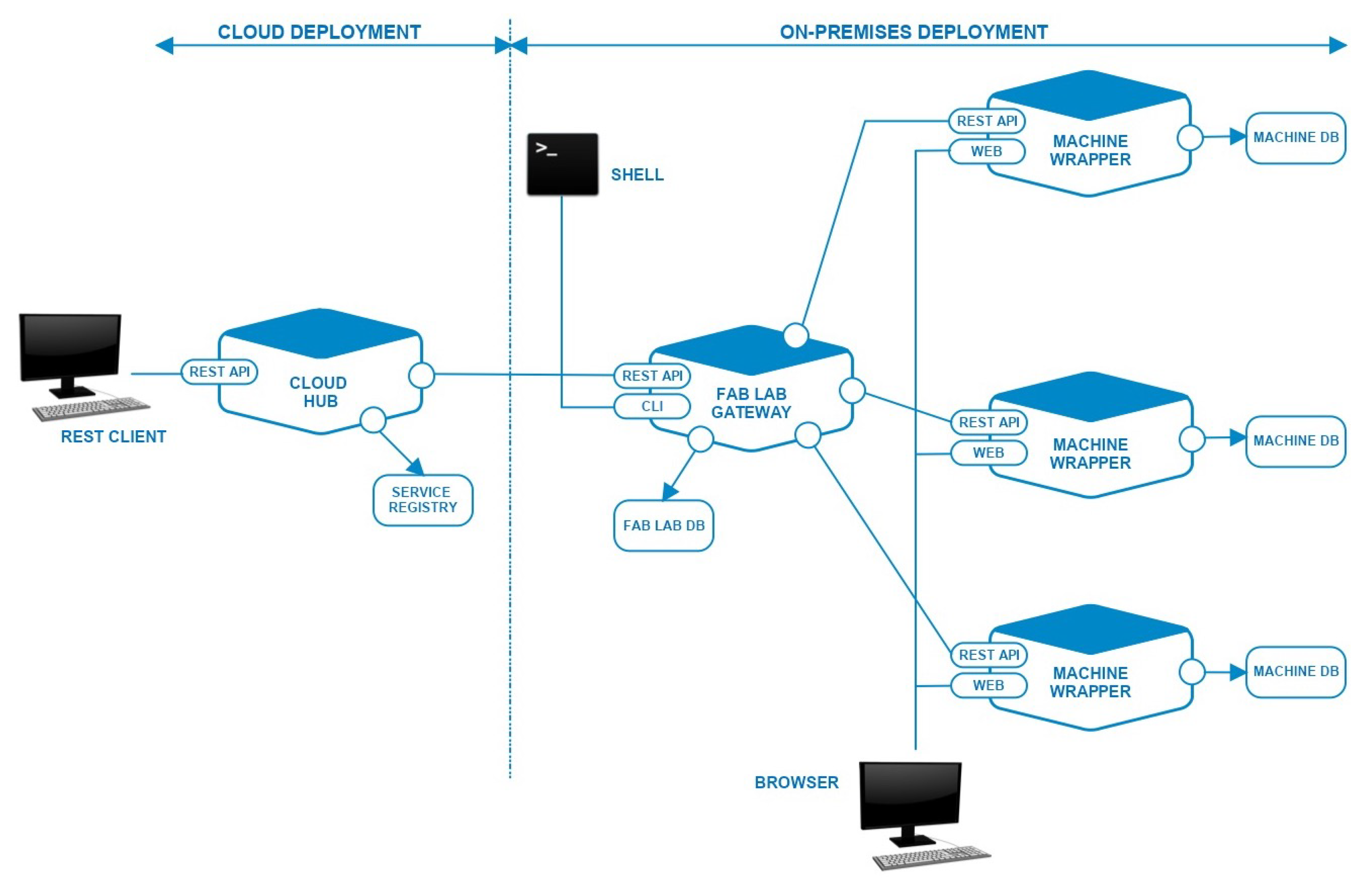
As mentioned before, the NEWTON Fab Lab platform has been designed as a set of loosely coupled microservices deployed both on premises and on the cloud as depicted in
Figure 1.
All the microservices that form the Fab Lab infrastructure communicate and interact through a set of REST APIs. Each microservice is relatively small and hence is easier to understand, develop, test and maintain.
Digital fabrication machines have no network connectivity; thus, in order to make them available over the internet as web services, we added an extra hardware and software layer (the machine wrapper) to provide each machine with external connectivity and communication protocols to interact with the Fab Lab gateway.
Both the Fab Lab gateway and the machine wrapper implementation rely on inexpensive off-the-shelf microcontrollers. The only restriction that applies to hardware choice is the capability to run a unix-like operating system and Node.js (
https://nodejs.org/) support. In fact, lately Node.js has become a de facto industrial standard for the development of real-time distributed embedded system and IoT applications [
12,
13,
14].
In the case of the NEWTON platform, Fab Lab gateway and machine wrappers have been implemented using Raspberry Pi embedded computers, for this reason we will refer to them also as Pi-Gateway and Pi-Wrapper, respectively.
In the following subsections we will describe in depth all the principal hardware and software components that form the NEWTON Fab Lab platform.
2.1. Cloud Infrastructure
As stated earlier, the NEWTON Fab Lab platform implements a spoke-hub architecture in which the hub node, located on cloud premises, acts as a router forwarding the fabrication requests to the selected Fab Lab.
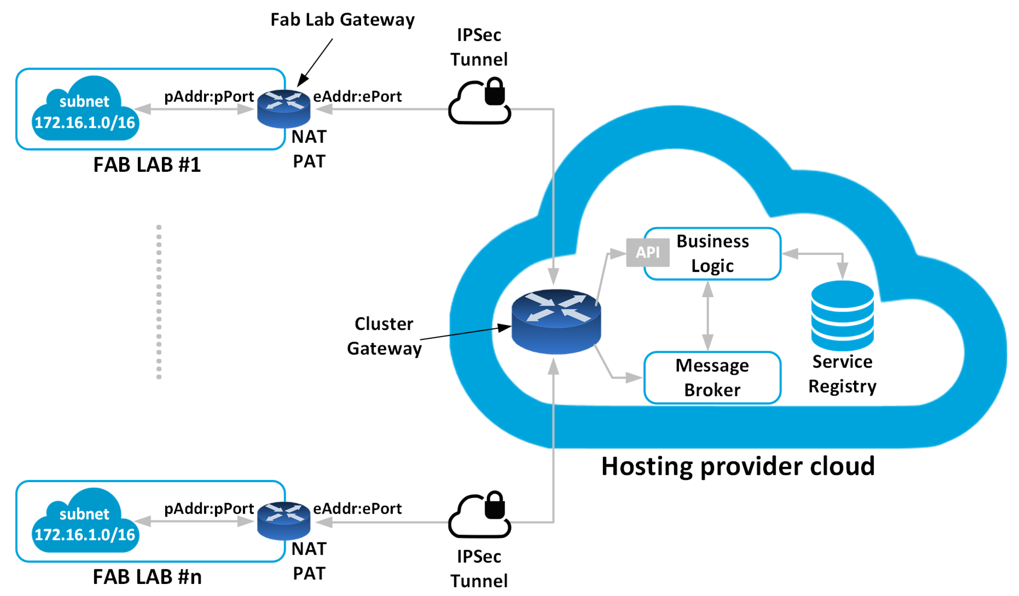
Figure 2 shows the simplified Fab Lab network architecture.
The NEWTON Fab Labs employ a two-tier architecture composed of a hub and a network of distributed Fab Labs. Each Fab Lab interacts with the hub and other labs via a Fab Lab Gateway. While some novel Internet of Things architectural paradigm exists, in which some data processing is performed at the edge of the network by the devices themselves [
15], we have preferred a standard approach with all the data to be processed directly in the cloud. This is because the amount of data to be processed (i.e., the Fab Lab status) is not large enough to justify an extra middleware layer between the Fab Labs and the Cloud hub.
Each Fab Lab is exposed as services to the Internet through REST APIs that provide Create, Read, Update and Delete (CRUD) methods to manipulate the underlying data model as well as communication primitives to publish and subscribe to services over the Web. The Service Oriented Architecture (SOA) guarantees the inter-operability of the different system components, regardless of the implementation technology and allows easy system scalability. The service registry is held on cloud hosting premises and keeps the status of all the interconnected Fab Labs.
Spoke and hub nodes form a Virtual Private Network (VPN) in which the Fab lab gateway and the virtual machine instances on cloud premises communicate securely over the internet using private IP addresses though an IPSec (IP Secure) tunnel.
IPsec is a suite of protocols for managing secure encrypted communications at the IP Packet Layer. IPsec also provides methods for the manual and automatic negotiation of security associations (SAs) and key distribution. A security association is a unidirectional agreement between the VPN participants regarding the methods and parameters to use in securing a communication channel. Bidirectional communications require one SA for each direction. Through the SA, an IPsec tunnel can provide the following security functions:
Data privacy (through encryption)
Content integrity (through data authentication)
Sender authentication and—if using certificates—non repudiation (through data origin authentication)
The router/gateway maps the inbound traffic into a private address pAddr:pPort by means of a Network Address Table (NAT) and a Port Address Table (PAT). Similarly, the router performs the same task on the outbound traffic by forwarding it to the default gateway or by redirecting the requests for a private address to the private network. The message flow between the cloud application and the networked Fab Labs is managed by a cloud-deployed message broker that implement a publish/subscribe protocol.
2.2. Infrastructure Architecture and Modelling Challenges
Figure 3 depicts the simplified cloud infrastructure diagram of the NEWTON Fab Labs. For the sake of simplicity, the infrastructure necessary to connect the Cloud Hub to the Fab Lab network is not shown on the diagram. Analyzing the diagram of
Figure 3 leads to the conclusion that deploying a redundant implementation of the NEWTON Fab Labs cloud hub requires up to six levels of AWS services. This, in turn entails several challenges tied to infrastructure and application set-up, administration, and behaviour predictability. On one hand, the promise of scalability, redundancy and on-demand service deployment makes a cloud implementation a very appealing solution. On the other hand, all these advantages come at the price of several issues that can make cloud application development and management a challenging task.
More specifically, the issues with cloud deployment are related to the following impact factors:
Performance. Performance can become an issue in cloud development when it comes to disk IO. In a cloud infrastructure, the network and the underlying storage are shared among several customers. If, for example, another customer performs many IO operations, an application may experience slowdowns and its latency becomes unpredictable. Moreover, also the network is shared among customers, so one can experience bottlenecks there too.
Transparency. Transparency and simplicity are key factors when debugging either an application or an infrastructure. Unfortunately, cloud services are, in many cases very opaque and tend to hide underlying hardware and network problems. Cloud infrastructure is a shared service, and, for this reason, cloud users may experience issues that do not occur in dedicated infrastructure:
Impact of other users on your workload. In a cloud infrastructure, you share the underlying hardware resources with other customers. This includes CPU, RAM, disk and network. Cloud software attempt to isolate the resources allocated to each customer; unfortunately, the isolation is not perfect, and, in some cases, a single user can saturate a local compute node.
Service outage due to hardware errors. The software wrappers that expose the underlying infrastructure as a service may hide hardware failures that can only be confirmed by migrating an instance to another physical node. While cloud makes this migration straightforward, underlying physical failures can complicate the debugging process due to the lack of transparency.
AWS offers some solutions such as dedicated instances and dedicated hosts to improve the isolation from the infrastructure of other AWS customers and the latency of your cloud infrastructure; however, these services incur extra costs that it is not always worth assuming.
Complexity and scalability.
Figure 3 gives an idea of the complexity of the cloud architecture that has been deployed to ensure NEWTON Fab Labs connectivity. This entails the interaction of up to six different AWS service layers that require expertise for set-up and configuration. Moreover, Elastic Load Balancing and scalability are not straightforward in AWS and require the deployment and configuration of additional services (namely,
CloudWatch and
CloudFormation) that incur extra costs and complexity.
2.3. Global Infrastructure Deployment
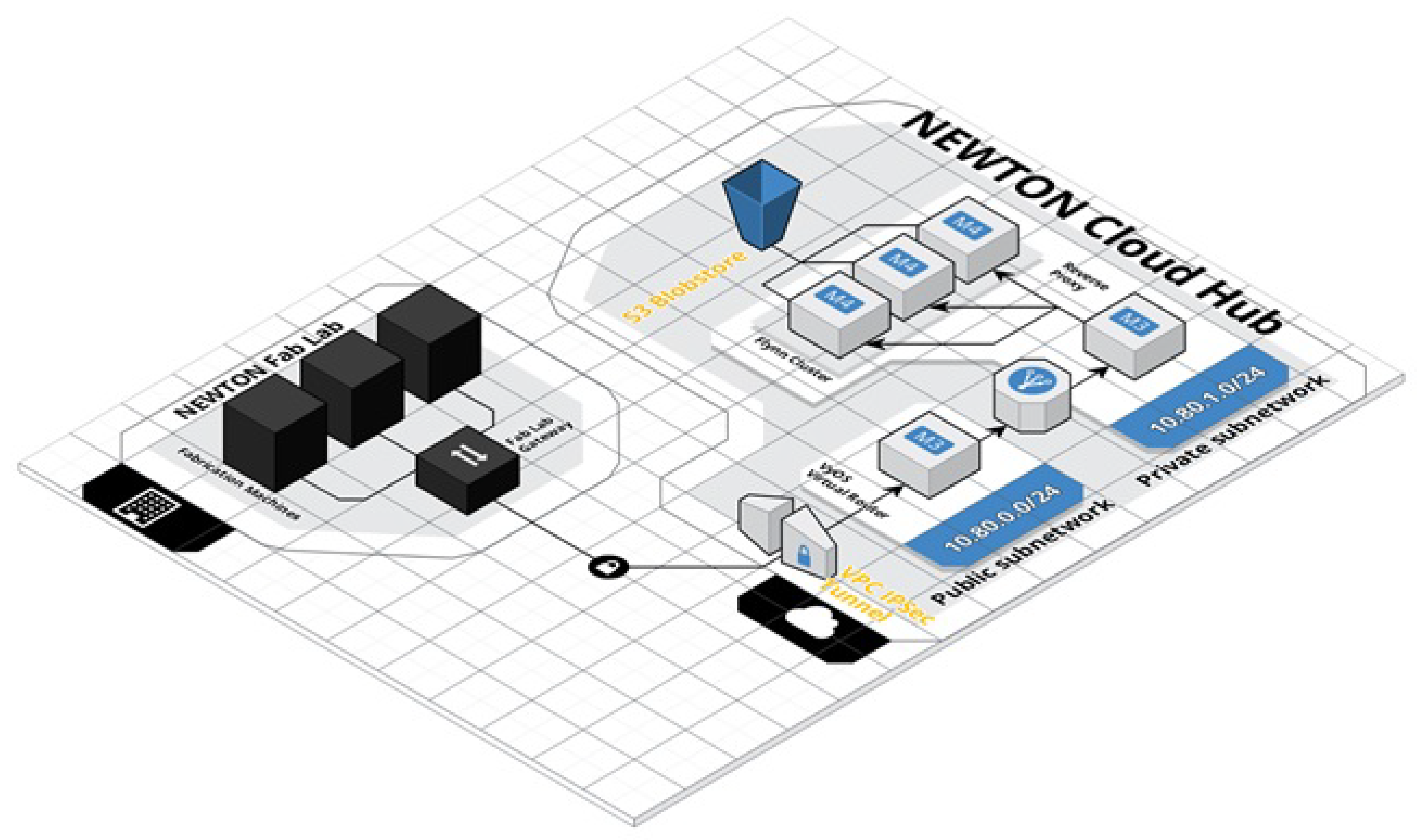
Each Data Center of the NEWTON Fab Lab Network is connected to a Fab Lab through an IPSec tunnel as depicted in
Figure 4.
On the cloud end, the IPSec tunnel is managed by a VyOS (
https://vyos.io) that acts as the bridge between the public and the virtual cloud subnetworks forwarding all the incoming packets to a reverse proxy/load balancer that eventually delivers the incoming request to the cloud hub application. Both VyOS and the reverse proxy run on dedicated m3.medium EC2 instances.
The cloud hub application and all the related services are deployed on a PaaS infrastructure implemented by a Flynn (
https://flynn.io) cluster formed by three m4.large EC2 instances. All the applications run in Docker containers. Docker images are stored using AWS S3 cloud storage.
Thus, with this architecture, the latency of a fabrication request can be split into four parts:
The latency of the POST request from the client to the spoke or hub (depending on the region in which the requesting client is located).
The latency of the request to the service registry (this delay may vary depending if the request has been performed from the hub or from a spoke node).
The latency of the POST request from the spoke or hub to the selected Fab Lab.
The latency of the POST request from the spoke or hub to the client.
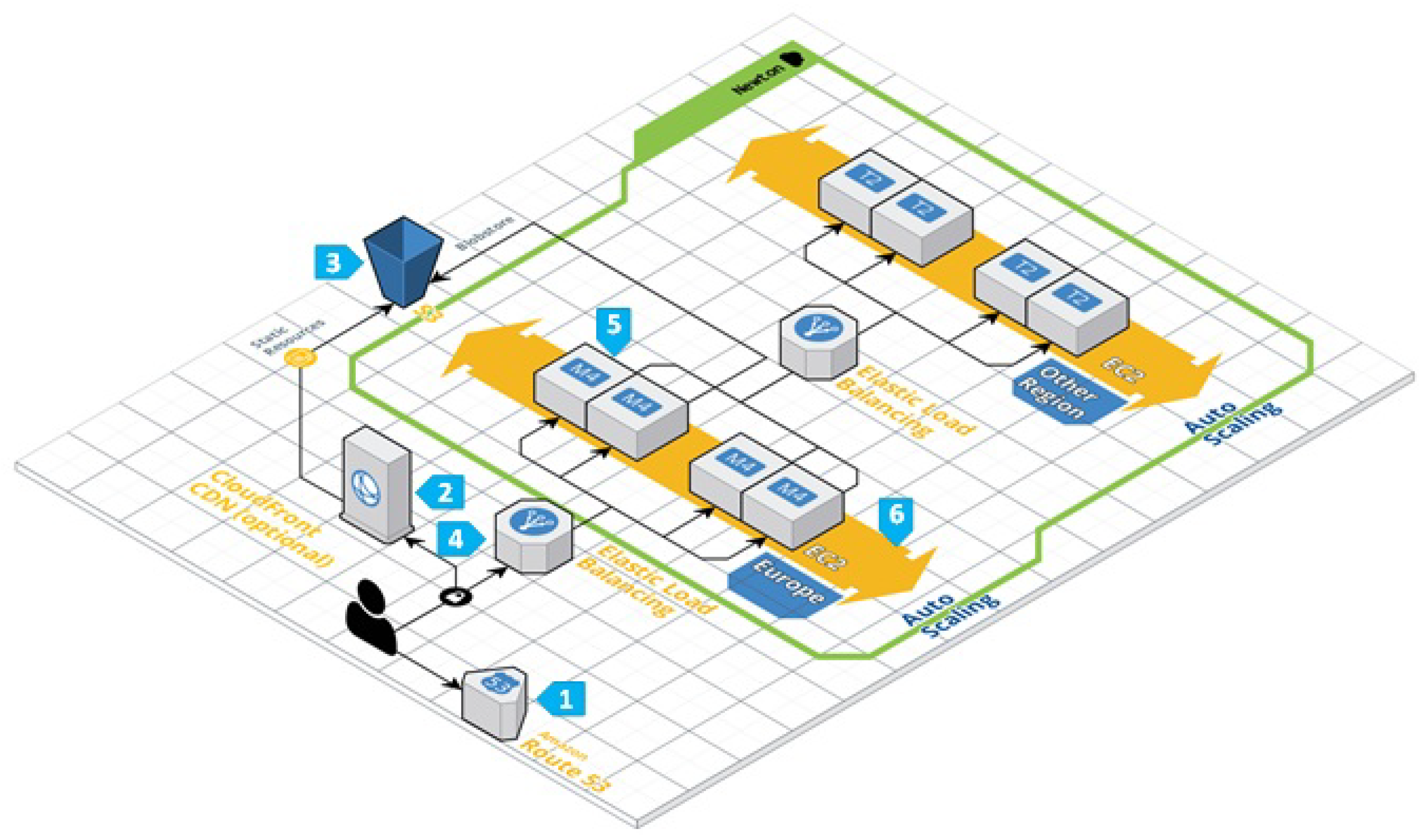
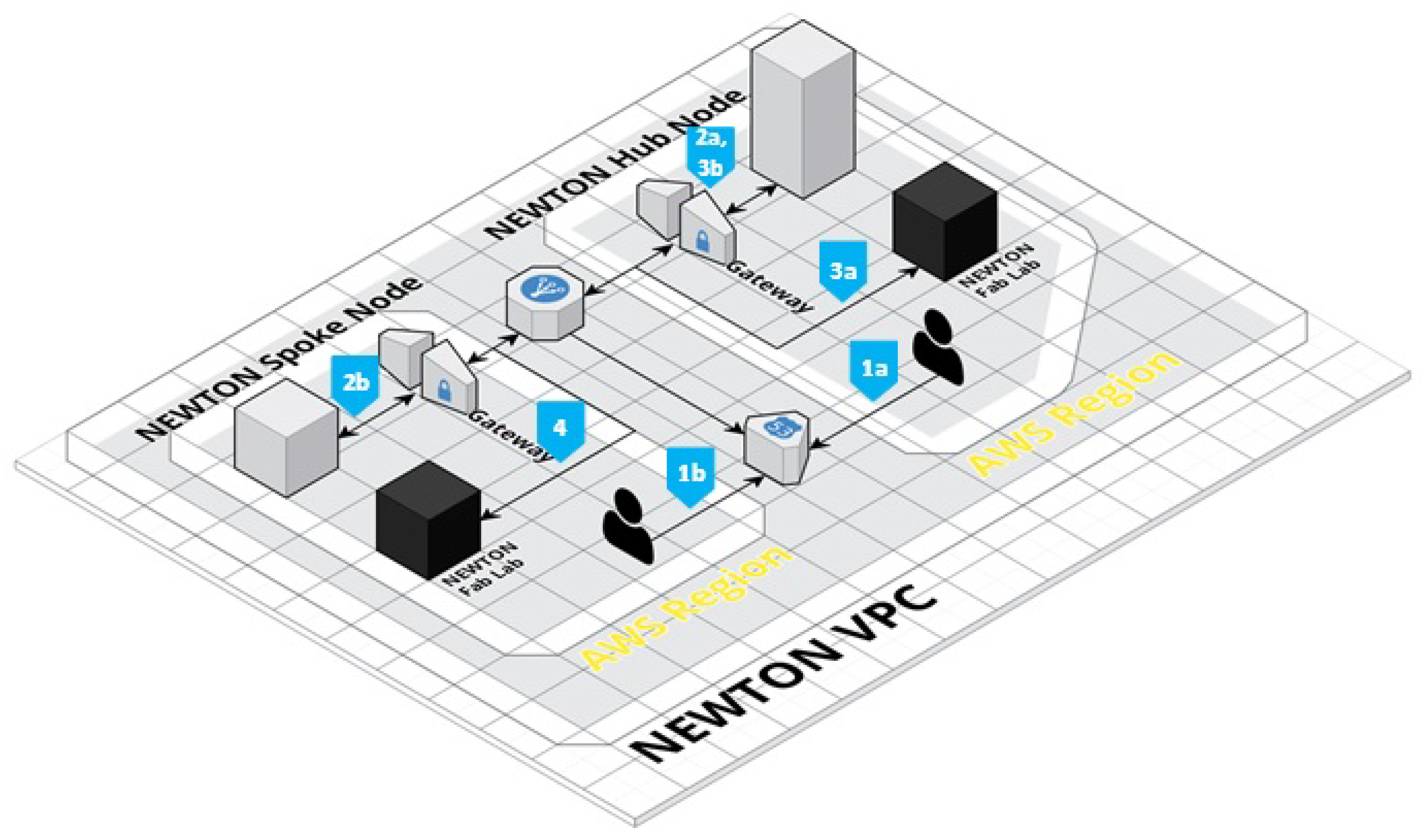
This scenario is depicted in
Figure 5 that shows how the fabrication requests are routed within the NEWTON Amazon Web Services (VPC). NEWTON VPC comprises several AWS-supported regions where hub and spoke nodes infrastructure is deployed.
2.4. Some Remarks on Production Deployment
NEWTON Fab Lab network infrastructure under test is distributed over four Data Centers located in different AWS regions (eu-central-1, us-east-1, sa-east-1, and ap-southeast-1). The network implements a spoke-hub architecture whose central hub is located in the eu-central-1 region (Frankfurt). The hub runs the Fab Lab monitoring application and the registry server that keeps track of the status of all the interconnected Fab Labs.
The spokes run light clients that connect to the central hub to inquiry the registry server and then forward the fabrication job to the closest Fab Lab in their region. This approach limits the heavy traffic (i.e., the images with the design to be processed by Fab Labs) only within the AWS region where the fabrication request is generated.
In our measurements we set-up the Data Centers network using isolated VPCs (Virtual Private Clouds) communicating through public IP addresses. While this approach is not a concern in a test environment, it is not advisable in a production set-up. AWS offers the possibility to create out-of-the-box secure peer connections among different Data Centers forming a VPN (Virtual Private Network) in which the interconnected Data Centers communicate using private addresses.
The requests are routed by the AWS Route 53 service to the NEWTON data center (either the hub or a spoke) that falls in the same AWS-supported region of the requesting client (steps 1a and 1b of
Figure 5). If the request is forwarded to a spoke node, the spoke queries the registry server located in the hub to get the location of the NEWTON Fab Lab that is geographically closer to the requesting client (step 2b). The hub returns to the spoke the requested information (step 3b) and finally, the spoke forwards to the selected Fab Lab the fabrication request and the design files (step 4).
If the incoming requests comes from a client within the same Hub node region, the request and the design files are forwarded to the Hub (step 2a) and it is the Hub business logic that queries the registry server to get Fab Lab information and then forward the request and the design files to that Fab Lab (step 3a). With such an approach, we limit the heavy traffic among data centers in different AWS regions since the design files are always kept in the VPC node closer to the requesting client.
2.5. Communication Protocol
A fabrication job is routed to a networked Fab Lab by the Cloud Hub message broker; however, the message broker on the cloud side has not direct visibility of the Fab Lab network infrastructure. Its main task is to connect a client to the Fab Lab infrastructure or to perform inter-Fab Labs message routing. The networked machines in a Fab Lab can be accessed through the Fab Lab Gateway only. The gateway main task is routing the outbound traffic to the networked equipment and managing intra-Fab Lab communications.
The communication between the cloud infrastructure and a networked Fab Lab is performed in the following for stages:
link establishment;
topic subscription;
communication;
disconnection.
Once the TCP (Transfer Control Protocol) links between the machine and the Fab Lab Gateway on one side, and the Fab Lab Gateway and the Cloud hub broker on the other side, have been established, both the Gateway and the Hub subscribe to topics they are interested in. The topic string is generated using the unique name and connection ID sent by the server that initiates the communications to the destination server during the link establishment. Both the link establishment and the subscription phases are terminated by an ACK message (Init ACK for the link establishment and Subscription ACK for the subscription phase).
In other words, the Fab Lab Gateway and the Cloud Hub implement, as mentioned before, a double broker architecture: The former collects all the incoming messages from the Fab Lab machines whereas the latter collects all the incoming messages from the networked Fab Lab Gateways. The double broker architecture allows the implementation of Fab Lab access and security policies and of custom message filters mechanisms. Once the subscription phase has terminated, the end nodes start exchanging messages. Each published message can be acknowledged by an optional Publication ACK message. The use of a Publication ACK is mandatory in those cases when it is necessary to guarantee the delivery of a message and to implement retransmission mechanisms to increase the QoS of protocol.
3. Simulation Model and Data Analysis
The simulation model is of paramount importance to analyze the performance of the NEWTON Fab Lab platform under different load conditions in order to determine the factors to consider when scaling the platform infrastructure. Scaling is a necessary action that must be performed in order to ensure the desired quality of service (QoS) as the system load increases. The number of concurrent users and the number of submitted jobs per user determine the system load.
Scaling can be either vertical (i.e., by increasing the computing power of each node in terms of CPU, RAM etc.) or horizontal (i.e., by increasing the number of nodes that form the platform). NEWTON Fab Lab platform has been designed to scale horizontally by leveraging the autoscaling service provided by the Amazon Web Services (AWS) cloud infrastructure.
The modelling process goes through two steps:
first, we define a set of metrics and then choose only the most relevant ones; namely, those metrics relative to the technological and workload factors that have the greatest impact on system performance;
then we then design a set of experiments to stress the system performance with different resource allocations and workloads.
3.1. Cloud Deployment
NEWTON Fab Lab platform is a distributed hardware/software platform formed by several interconnected Fab Labs exposed to the internet as web services through a Fab Lab Gateway. Inter Fab Lab communication is managed through a centralized cloud hub that keeps in a service registry the state information of all the interconnected Fab labs. Moreover, the cloud hub also exposes some APIs to submit and manage fabrication batches to the NEWTON Fab Lab platform.
The capacity of the platform to scale (i.e., the capacity to manage a high number of interconnected Fab Labs and users) tightly depends on the scaling capacity and efficiency of the cloud infrastructure. For this reason, we will target only the scalability issues related to the cloud infrastructure and not those of an individual Fab Lab. NEWTON Fab Lab platform is formed by a set of distributed nodes in different Data Centers, each node is a virtual machine characterized by:
Several nodes can be interconnected to form a grid of load-balanced containerized services and applications. The minimum cluster requirements for a deployment on AWS (Amazon Web Services) cloud infrastructure are depicted in
Table 1. More specifically,
Table 1 depicts the minimum hardware requirements necessary to deploy a Flynn cluster in production.
An AWS m4.large instance has two virtual CPUs 8 GB memory and runs an Ubuntu 16.05 (Xenial) Linux distribution. NEWTON Fab Lab cloud hub is hosted on an AWS Data Center in Frankfurt and comprises a set of three load balanced m4.large EC2 (Elastic Cloud Computing) instances with 600 GB disk each. The cloud hub hosts a PaaS (Platform as a Serivice) infrastructure. that allows the deployment and orchestration of containerized application and services. The deployed application and services communicate with the remote clients through the internet and with the networked Fab Labs with dedicated IPSec tunnels. The traffic between the client and the cloud application and between the cloud application and the networked Fab Labs is variable and may vary between few hundred bytes (in the case of a simple API call) and some MBytes (when a design image is submitted for fabrication).
3.2. Available Services
The NEWTON Fab Lab cloud hub runs the following services:
Platform orchestration and management services (Docker container orchestration, platform dashboard, logging system, GitHub connector, databases, etc.)
Fab Lab related services (registry server, fab lab APIs)
3.3. Service Containerization and Scaling
All the services running on the allocated virtual machines are deployed in Docker containers orchestrated by a PaaS (Platform As a Service).
The PaaS infrastructure is deployed on top of Flynn (
https://flynn.io). Flynn can be considered as a grid of Docker containers, rather than a traditional cluster. Each host will run containerized services and applications that can be deployed and scaled individually.
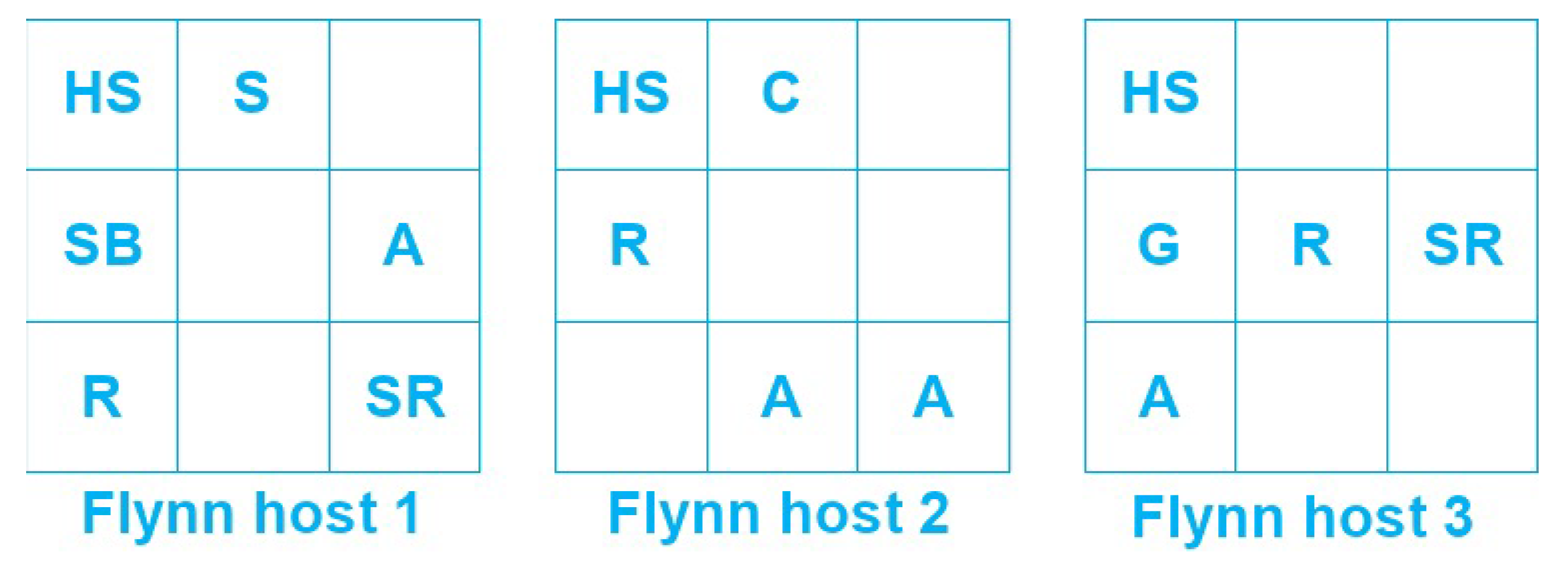
Figure 6 shows a simplified diagram depicting a Flynn grid deployment across a cluster of three hosts.
Flynn architecture is split into two layers. Layer 0 provides basic services such as host management, service discovery and scheduling, whereas layer 1 implements the PaaS business logic (GitHub interface, Slug Builder, Slug Runner, etc.). Referring to
Figure 6, the layer 0 services are:
The Host Service (HS) that implements the interface between Flynn services and Docker. The Host Service is the only one that must run across all the Flynn hosts
The Scheduler (S). The scheduler distributes the containers among the instances given the current state of the grid and the resource allocation in each node.
The layer 1 services are:
The GitHub frontend (G). This module accepts Git connections through SSH and Git pushes, then deploys them in the Flynn grid.
The Controller (C) exposes APIs to control the whole infrastructure.
The Router (R) is a TCP/HTTP router/load balancer that distributes the incoming requests through the instances deployed in the Flynn grid. In order to implement a high-availability there must be several instances of this module across all the Flynn hosts.
The Slug Builder (SB) is a module that builds a “slug” starting from a Git push received by the Flynn Git front-end (G). A slug is a compressed and pre-packaged copy of an application optimized for distribution to the Flynn PaaS.
The Slug Runner (SR) is a module that allocates and instantiates several Docker containers (depending on the scaling parameters) to deploy and execute the code contained in a slug.
The Application (A) is a module that implements the application code (for example, the Cloud Hub and the Service Registry in our specific case).
While this solution provides seamless scaling and monitoring of all the services running on the cloud infrastructure as well as GitHub integration that allows the deployment of an application from a GitHub repository, it also has some drawbacks. The Docker engine is tightly integrated into the PaaS infrastructure and cannot be accessed through Docker commands but only through the PaaS. This means that a user has no control on the container structure and the allocated resources, that are seamlessly managed by the PaaS infrastructure. This, in turn, makes hard to know exactly the hardware resources that are allocated to a container by the PaaS. Consequently, the only way we have to estimate the kernel memory allocated to a container is by using the free –m Linux command. Considering that a m2.large instance has 8 GByte RAM, that Ubuntu 16.05 requires between 1 and 2 GByte memory in order to operate efficiently, and that the free –m command leads to an estimation of 20 MByte of kernel memory per container, the estimated memory allocation for our containerized infrastructure is that reported in
Table 2.
3.4. Test Infrastructure Set-up
To test the bandwidth among the hub region eu-central-1 (Frankfurt) and spoke regions us-east-1 (N. Virginia), ap-southeast-1 (Singapore) and sa-east-1 (Sao Paulo) we set up the following test infrastructure:
One t2.micro test instance in us-east-1 region,
One t2.micro test instance in ap-southeast-1 region,
One t2.micro test instance in sa-east-1 region.
To test the bandwidth among the instances in the central hub and the test instances in the spoke regions we follow AWS recommendations and use iPerf3 (
https://iperf.fr) network benchmarking tool.
The virtual machines must allow inbound traffic on port 22 (SSH), TCP traffic on the iPerf3 server (in our test configuration we run iPerf3 servers on port 80) and, optionally, allow ICMP traffic.
Measurements have been performed ten times at random intervals for all the spoke regions and within the hub region. At each iteration, we measure the average bandwidth, the median, the variance, the fastest and the slowest connection bandwidth for both up and downlink connections. The results are summarized int
Section 4.
3.5. Performance Key Factors
So far, we have defined the system features and architecture and identified the services that run on the system under study. In order to build a simulation performance model and to define the experiments we want to carry out with it, we must consider application scalability within a cluster, cluster scalability within a Data Centre, and platform scalability considering the impact of multiple Data Centres distributed on a wide geographical area.
Application scalability is affected by the number of containers allocated to it; cluster scalability is affected by the number of virtual machines allocated to a cluster. Finally, platform scalability across multiple Data Centers if affected by the geographical origin of the service request. The data attached to a fabrication request can be either a .gcode file (namely, a simple text file with machine commands) or a .png file (i.e., an image file with the shape to be fabricated). However, in both cases the data interchanged during a fabrication request can be considered constant. For the sake of simplicity, we assume that an image of 5 MB size (i.e., a typical image size for a slightly complex design) is attached to each fabrication request. The key factors to be evaluated in the study must also reflect the features offered by the Cloud Infrastructure Provider (Amazon AWS in our case). More specifically, we want to develop a model that takes into account the Autoscaling and Elastic Load Balancing features offered by AWS infrastructure. The autoscaling is the capability of dynamically scaling up or down the computing infrastructure according to the value of a given performance metric. Thus, the key study factor will be the metric that will trigger infrastructure scaling (either up or down). In our case, scaling will be triggered by the system workload, i.e., by the number of incoming requests. Moreover, the cloud infrastructure must ensure that incoming requests are evenly distributed among Data Centers while ensuring maximum geographic coverage. This, in turn, means that the number of Data Centers must be constant and encompass all the AWS supported regions. To summarize, we will keep constant the following parameters:
Characteristics of the virtual machines.
Size of the transferred data.
Number of Data Centres allocated to the global infrastructure.
We will not consider network reliability and packet retransmission due to their extremely low impact on overall system performances. Today’s network infrastructure is very fast and reliable and the number of retransmissions due to noise and packet losses is extremely low and close to 0%. In addition, we will consider data transfer with a fixed size. Thus, the only key parameters in our experiments will be the:
We will stress system performance varying these parameters under different load conditions (i.e., varying the number of connected users as well as their geographic origin) while keeping constants all the other parameters.
3.6. Evaluation Technique
NEWTON Fab Lab platform is a complex distributed infrastructure that relies on many subsystems deployed both on cloud and on Fab Lab premises in order to allow Fab Lab communications and integration with third-party applications and infrastructure. During the developments described in [
11] we have deployed a minimum infrastructure and stressed it in real operating scenarios through several test pilots described in [
8,
9,
10]. We also performed several load tests under different simulated load conditions to measure the APIs response times and have a more accurate idea of the overall system performance. However, these measurements are just a starting point since have been obtained for a particular deployment. In the future, the number of interconnected Fab Labs and consumer applications is supposed too scale up which, in turn will imply the allocation of new cloud resource to manage the new use-case scenarios. For this reason a simulation model of the Fab Lab infrastructure is necessary in order to estimate how many resources (i.e., virtual machines and docker containers) it is necessary to allocate in order to ensure the target quality of service; namely, to ensure that system response times under all the assumable load conditions falls below a given limit established
a priori by the platform administrator. In order to evaluate NEWTON Fab Lab platform performance, we proceed in two steps:
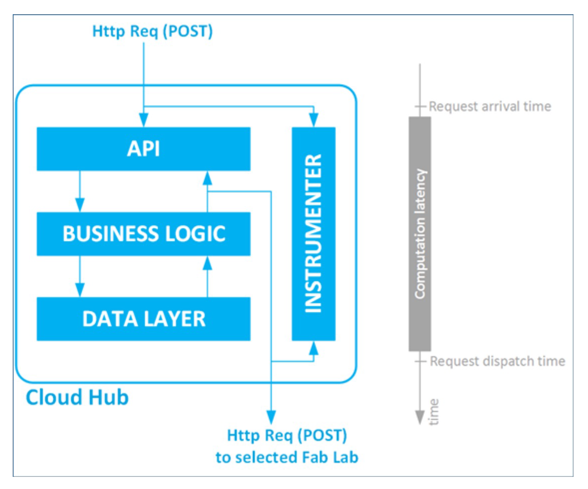
We stress the real cluster deployment using a fake client to simulate user behaviour issuing a fabrication request 10 times at random intervals comprised between 1 and 30 s. The cloud hub application has been instrumented as depicted in
Figure 7 to measure the elapsed time between the arrival time of a fabrication request and the dispatch time of that request to the selected Fab Lab. We perform the measurements under different load conditions generated by
n concurrent users (where
n is a power of two included in between 1 and 64) for a variable number
c of Docker containers (where
c is a power of 2 with
) allocated to the Cloud Hub application; then, we use the measured data to build a simple consistent analytic model of the cluster performance based on linear regression.
We use the predictive model built at the previous step to define a mathematical model of a Data Center; then use this model within CloudSim cloud simulator to evaluate platform scaling and reliability under different load conditions. The CloudSim software model we have developed mimics Amazon AWS Autoscaling and Elastic Load Balancing (ELB) features across several availability zones; thus, the incoming requests are dynamically routed to the Data Center of the global infrastructure that is closer to the issuer of the request. Furthermore, the resources (i.e., the number of virtual machines) available in each Data Center are dynamically allocated (either scaled up or down) depending on the number of incoming requests.
3.7. Cloud Hub Modelling
Table 3,
Table 4,
Table 5 and
Table 6 summarize the statistical distributions of the measured system latencies for several application set-ups. For each set-up, the mean, median, minimum and maximum value as well as the standard deviation are reported. The 50% of the incoming requests are served in between the minimum and the median time; whereas the remaining 50% of the requests are served in between the median and the maximum time. However, the mean response time is very close to the median and standard deviation very high, which clearly denotes, as expected, a non-normal tail distribution of the measured data. In addition, the measured data seems loosely correlated to the number of requests and the number of containers allocated to the application, which makes very difficult to make reliable predictions of the Cloud Hub application latency. Lognormal and Pareto distributions are those that better model server response time [
16]; in fact, the measured data matches with very good accuracy a Pareto distribution. Observing the tables, we note that the minimum and median delay values decrease as expected (with some outliers) as the number of allocated containers scales up; however, this is not the case for the maximum values. As highlighted by Downey [
16], this is a typical behaviour of internet applications. In our specific case, this high variability is due to the performance impact factors of the cloud infrastructure that add an unpredictable latency to cloud-deployed applications as outlined in
Section 2.2. We have performed our measurements at random times explicitly to trigger this variable behaviour and the effect of the other Amazon AWS customers application load on the performance of our infrastructure. However, recall that the impact of the maximum delay on the overall performance is minimum; since, in a tail distribution the probability of high delay is very low.
We choose to model the server response time with a simple Pareto (type I) probability density function:
where
is the shape parameter and
is the scale parameter of the distribution. An estimation
of the scale parameter can be computed as:
where
represents the value that can be assumed by the random variable
X. In our specific case, the random variable
X represents the server latency and the measurement
can be considered as a function of the number of requests
r and the number of containers
n allocated to the cloud application; namely:
A simple estimation
of the minimum latency measurement
for a given number
r of incoming requests and number
n of containers can be obtained using a multiple linear regression on the measured data set reported in
Table 3,
Table 4,
Table 5 and
Table 6, leading to:
with
and
.
For practical reasons, we have limited the evaluation space to and respectively. Consider that with this set up we perform 1270 requests to our cloud infrastructure at random times comprised within 0 and 30 s; this means that, in the worst case, a measurement can take almost 11 hours. With this approach, we trade simplicity for accuracy since, as outlined before, cloud customers share hardware and network resources, which makes the latency of the cloud infrastructure hardly predictable. In fact, the parameter for the simple prediction model is 0.45. The coefficient of determination is the ratio between the explained variation and the total variation of a dependent variable; in other words, it is a statistical measure of how close the observed data is fitted to the regression plane . Thus, means that our simple predictive model only covers the 45% of the observed values. However, the parameter does not indicate whether a regression model is adequate or not. You can have a low coefficient of determination for a good model, or a high coefficient of determination for a model that does not fit the data.
An estimation
of the shape factor
can be computed as:
where
represent the geometric mean of the measured values
.
However,
is a function of the number
r of incoming requests and number
n of containers; thus, also the shape factor estimation
is a function of those parameters. This leads to:
In this case too, the estimation
can be derived from a multiple linear regression on the measured data set reported in
Table 3,
Table 4,
Table 5 and
Table 6, leading to:
with
and
.
Additionally in this case the coefficient of determination is low (, which implies on an 18.2% coverage of the measured values). We use the estimations of the scale parameter and of the shape parameter to generate the cloud servers’ latency for different values of r and n in our simulations.
Given a uniform random variable
, a latency
with a Pareto distribution can be generated as:
Recall, that the proposed scheme does not predict the latency of the cloud-deployed servers; this would make no sense, since, as stated before in a cloud environment several customers share the same network and infrastructure which makes very hard to predict the server behaviour in a given instant. What we do instead, is using the measured data to predict the shape of the Pareto distribution that models the performance of our cloud infrastructure under different load conditions and number of allocated containers. We then use this prediction to generate, in our simulator, a random latency with that Pareto distribution starting from a uniform random variable
U using Equation (
8).
3.8. Delay Model
In order to build a realistic simulation model we need to estimate communication latency and bandwidth among the nodes that form the Fab Lab network as well as the maximum concurrency level that each node can support. This goal is accomplished through the following steps:
We estimate the network latency from client to Data center j and Fab Lab to Data Center j in the same AWS region. To do this, we use the real measurements provided by RIPE Atlas network. RIPE Atlas is a public network located in the last mile and formed by more than 16.000 measurement probes capable of measuring connectivity between internet endpoints on demand.
We estimate the network uplink and downlink bandwidth between client and Data Center
j (
and
respectively) and Fab Lab and Data Center
j (
and
respectively) in the same AWS region. To do this, we use the Clouharmony speedtest service (
https://cloudharmony.com/speedtest). However, this service allows measuring the desired parameters only between the client browser and the target Data Center. This means, that we are able to track performance only within Europe and must make the simplifying assumption that the network performances within the same AWS region are approximately the same using the measurements performed in Europe as the reference values.
We measure the Data center i to Data center j network latency using ping and traceroute. Traceroute is even better than ping since it allows testing the response time of each network segment along the path. Therefore, this tool can not only measure but also locate the latency across the routers that form the packets path.
We measure the Data center i to Data center j uplink and downlink bandwith ( and respectively) using iPerf3 tool.
The delay
D of the system response after a fabrication (POST) request has been issued is computed as follows:
where
j denotes a Data center located in a spoke node, whereas
k denotes the Data center located in the hub node. The delay
D of a response is hence the packet round-trip time necessary to follow the path the goes from the client to the spoke node, from the spoke to the hub node and then to the spoke again, from the spoke to the selected fab lab and then to the spoke again, and finally to the client.
Observe that the data transfer time
between nodes
i and
j in Equation (
9) is computed as:
where
and
represent, respectively, the number of bytes transmitted and the measured bandwidth between nodes
i and
j.
3.9. Concurrency Level
We use Apache Benchmark (
https://httpd.apache.org/docs/2.4/programs/ab.html) to estimate the maximum concurrency level that can be effectively borne by a node of the NEWTON cloud infrastructure. This allows us to estimate the maximum number of concurrent requests that can be served by the cloud infrastructure and to configure suitably the simulator that models NEWTON Fab Lab infrastructure.
The Cloud Hub APIs provide a root (‘/’) endpoint that supports both HTTP and HTTPS protocols and returns a response with a 200 status code and a body with an empty JSON (JavaScript Object Notation) object. We use this endpoint to ping the Cloud Hub sever; however, we can also use the same endpoint to perform simple load tests on our infrastructure. Nonetheless, you have to keep in mind that the result obtained in this way are optimistic since the authentication server and the underlying data base are not stressed. While Apache Benchmark tool generates very detailed reports, we are only interested in detecting which is the maximum number of concurrent requests that breaks our server leading to a timeout error. In order to do this, we stress our server during a prolonged period with an increasing number of concurrent requests until it breaks.
Table 7 summarizes the percentiles measured when a minimum cloud deployment (with only one container allocated to the cloud hub application) is stressed by 20,000 requests with concurrency levels 10, 50 and 100 respectively.
Observing the percentiles of the measurements, we note that in all the scenarios under test the response delays exhibit a tail distribution. In addition, increasing the concurrency level of the incoming requests leads to larger tail delays, being 100 the maximum concurrency level that can be supported by the cloud configuration under test. However, the measurements carried out are qualitative and are only useful to set-up our simulation model with reasonable values. In fact, the measurements performed have been carried out just for a short period of time, thus they do not take into account the delay variability of the cloud infrastructure as pointed out previously. Moreover, the measured times refer to the response latency for a simple API endpoint that returns a 200-OK response; consequently, they do not take into account the extra latency to access to the underlying data base to retrieve the Fab Lab information. For all the aforementioned reasons, it seems reasonable to assume that, in a real deployment, the Fab Lab infrastructure can support without problems up to 50 concurrent accesses and manage approximately 1000 requests per second (by scaling up the number of containers allocated to the cloud application).
3.10. Simulator Architecture
We have built a simulator on top of CloudSim [
17] in order to estimate the Fab Lab Network performance in several operating scenarios. We use the mathematical model developed in
Section 3.7 to estimate the latency of the cloud infrastructure and the delay model described in
Section 3.8 to estimate latency and bandwidth for Data-center-to-Data-center and Data-center-to-Fab-lab communication channels.
The simulation software has been built according to the the following hypothesis:
The CPU load of each instance of the cluster must not exceed the 50%.
The requests are evenly distributed among the cluster instances.
The incoming requests are evenly distributed within a given instance among blocks of 8 Docker containers, being 64 the container scaling threshold (This design choice is due to the fact that our prediction functions are defined for requests and containers. In addition, consider that Flynn does not natively support the container autoscaling feature implemented by our simulator. In order to enable container autoscaling you should use other container orchestration platforms such as DC/OS or Rancher instead of Flynn, provided you may afford higher deployment costs.).
The cluster minimum configuration can manage up to 50 concurrent accesses.
The pseudo-code snippet depicted in Listing 1 describes the block allocation and latency estimation process implemented by our simulator:
Listing 1.
Algorithm for estimation of cluster delays.
Listing 1.
Algorithm for estimation of cluster delays.
cluster_latencies = []
for (each instance in cluster) {
if (total_requests mod 64 != 0) {
allocate total_requests/64 +1 container blocks
} else {
allocate total_requests/64 container blocks
}
allocated_requests = total_requests/allocated_blocks
for (all the allocated blocks) {
compute Pareto scale param as (allocated_requests,8)
compute Pareto shape param as (allocated_requests,8)
cluster_latencies.push(compute_block_latency,())
}
} |
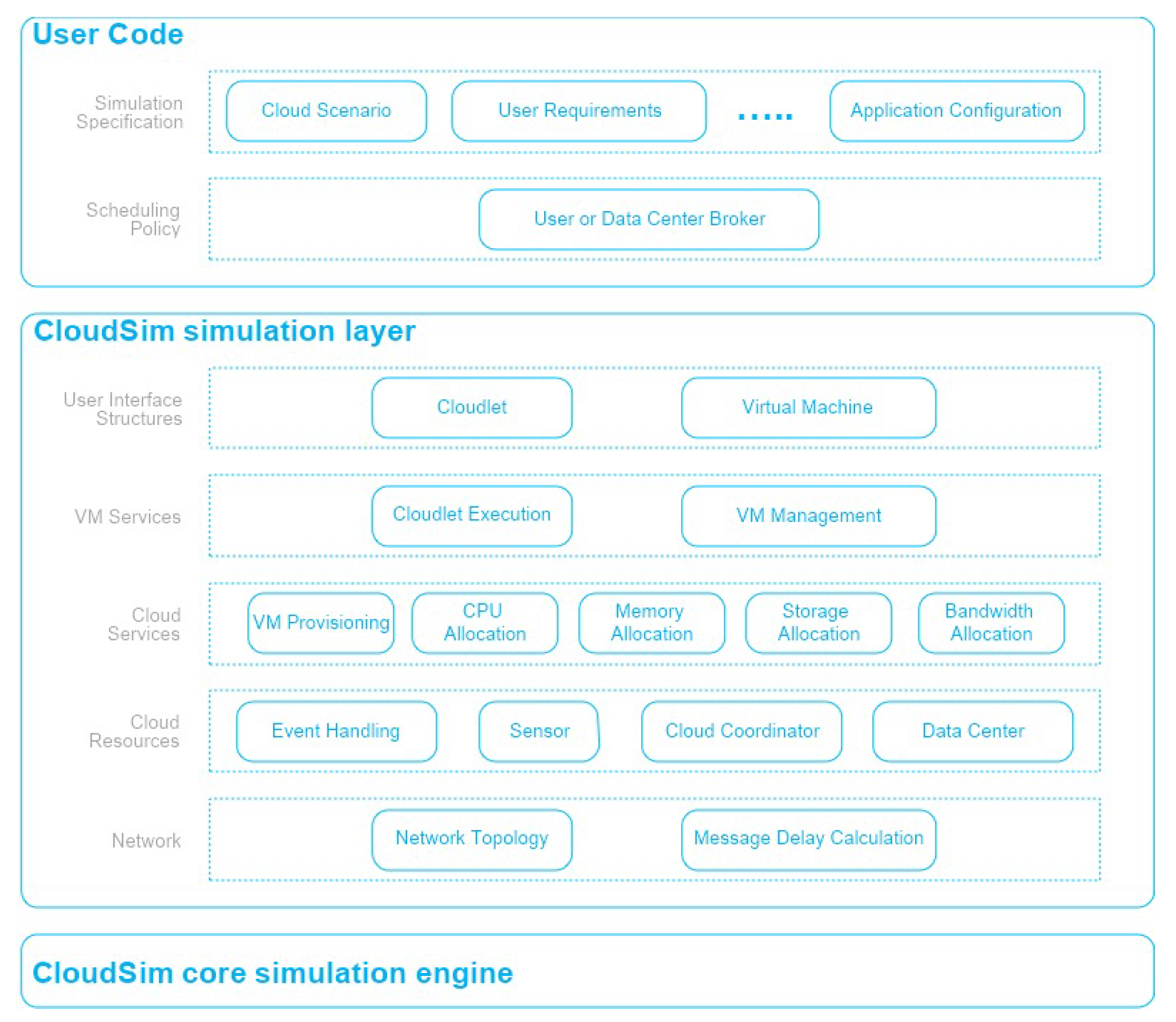
CloudSim simulator has a multi-layer architecture depicted in
Figure 8. The simulation layer provides classes and methods for simulation and modelling of virtualized cloud architectures. This includes dedicated management interfaces for Virtual Machines, memory, storage and bandwidth.
This layer also provides support for modelling Data center operation, such as Virtual machine host provisioning, application life cycle management, and system state dynamic monitoring. In addition, the simulation layer also exposes those functionalities that, like in our specific case, a Cloud application developer can extend to perform complex workload profiling and application performance study. CloudSim can be easily customized by implementing an extra software layer on top of the simulation layer. The User Code layer exposes basic entities for hosts (number of machines, their specification, and so on), applications (number of tasks and their requirements), virtual machines, number of users and their application types, and broker scheduling policies.
The User Code layer can be designed and configured in order to perform the following activities:
Generate a mix of workload request distributions, applications and configurations.
Model Cloud resources availability scenarios and perform robust tests based on custom configurations.
Implement custom application provisioning techniques for cloud infrastructure.
IaaS (Infrastructure as a Service) cloud infrastructure can be simulated by extending the Center class. The Data Center class is used by CloudSim to manage the host entities. Each host entity is assigned to one or more virtual machine according to the policies established by the Cloud Service Provider. More specifically, a virtual machine policy refers to all those operation and control policies related to a virtual machine life cycle within a Data Center. This includes virtual machine provisioning, creation, migration and destruction. In other words, a Data Center can manage several hosts that in turn manage several virtual machines during their whole life cycles. A Host is a CloudSim class that models a physical server (either single or multi core). Each host is characterized by its processing performance (expressed in millions of instructions per second or MIPS), as well as its memory and storage capability. A Host is also characterized by a provisioning policy to decide how many processor cores must be allocated to a given virtual machine. The allocation policy takes into account several hardware characteristics such as the number of available CPU cores, the CPU share and the amount of memory that is assigned to a given virtual machine. The core allocation operation is managed by a Scheduler component that implements by default either space-shared or time-shared allocation policies. The Scheduler class can be extended in the user program in order to implement custom CPU core allocation policies.
We have extended CloudSim to model and evaluate the performance under different load conditions of the NEWTON Fab Lab cloud infrastructure. More precisely, we modified the following CloudSim classes and configuration files:
Main class. We have defined the loops that run the tests and the simulation variables. In each iteration we call the runExperiment method. This method properly initializes all the CloudSim internal variables and classes. We do this through the following steps:
First, we initialize the CloudSim package.
Second, we create a set of four Data Centers: Datacenter_NorthAmerica, Datacenter_SouthAmerica, Datacenter_Europe, and Datacenter_Asia.
Third, we create a broker for each of the four Data centers. A broker is the CloudSim entity in charge of distributing virtual machines and cloudlets within the hosts of a Data center. A cloudlet is a representation of a task in CloudSim.
Fourth, we create a pool of virtual machines for each Data center and assign it to the Data center broker. The pool size varies dynamically between three and five depending on the number of incoming requests and mimics the AWS autoscaling function.
Fifth, we create a pool of four cloudlets (i.e., the CloudSim task) to manage the incoming requests and assign a cloudlet to each Data center broker. The cloudlets implement the pseudocode described in Listing 1.
Sixth, we define the cloud infrastructure topology that models the NEWTON Fab Labs and assign the CloudSim entities to each node of the networked Data centers.
CloudletScheduler. This class controls the distribution of the requests (managed by the cloudlets) in every virtual machine and estimate the time in which these jobs are accomplished. We calculate the execution times using the delay model described in
Section 3.8. To do that, we had to modify two methods of this class: updateVMProcessing and getEstimatedFinishTime. The former calculates the fraction of a job that is performed at a given clock tick, whereas the latter estimates the time remaining to complete this job.
DatacenterBroker. This class distributes the virtual machines among the hosts of a Data Center. This class has been suitably modified in order to deploy all the virtual machines managed by a given broker in its corresponding Data center.
Topology.brite. This is the file where the network topology is defined. In our specific case, the network has eight nodes (four Data centers and four brokers) and the edges that connect the nodes (six edges in our case: Three to connect the Data centers and three to connect the brokers). This file also specifies the distance between nodes and the bandwidth and delay that must be associated to each edge.
3.11. Design of the Experiments
Experiments have been designed to analyze the behaviour of the NEWTON Fab Lab infrastructure with the following users’ distribution: 250, 500, 1000, 1250, and 1500. Each user can issue from one to five requests; moreover, for each load configuration, the number of containers allocated to the application will scale as multiples of 8 from 8 to 128 (for a total of 16 possible configurations). These choices are basically driven by the need to reduce the number of iterations and hence the overall simulation time. Finally, the simulated infrastructure must cover requests from four AWS availability zones (Europe, North and Central America, South America and Asia-Pacific) in order to ensure a globally optimal service to all the world regions.
Table 8 summarizes the experiments’ configurations. The variable simulation parameters are the number of users, the number of requests per user, and the number of containers allocated to each instance of the cluster. All the other parameters are fixed. This means that for each possible user configuration 80 experiments must be performed (i.e., the number of requests per user times the number of possible container configurations). For the sake of simplicity, we also assume a uniform user distribution among different AWS regions.
Threshold is set to 1024 requests, i.e., the request count per target of each Elastic Load Balancing (ELB) target group must be kept as close as 1024 for the autoscaling group. More specifically, assume that you have configured an autoscaling group with a minimum of three instances (i.e., the minimum PaaS cluster configuration) and a maximum of six instances within an ELB group of a given AWS region. Setting a threshold of 1024 means that each instance of your cluster should receive approximately 1024 requests. If the overall number of incoming requests is larger, the number of instances should be scaled up to match the target threshold as close as possible. For example, if the cluster has three instances and the number of incoming requests is, say 3800, the system should scale up by one instance (i.e., from three to four), so that each instance handles 3800 / 4 = 950 requests. Finally, note that with the simulation set up depicted in
Table 8, the maximum number of incoming requests from a given region does not exceed 5000; thus, with a threshold of 1024 it makes no sense to have more than five virtual machines in the autoscaling group.
4. Results
Prior to running all the experiments, we have to make sure that the mathematical model we have developed for the cloud application behaves as expected. To do this we simply check that the simulated latency of the NEWTON cloud infrastructure matches a Pareto distribution. After running all the simulations whose set-up is detailed in
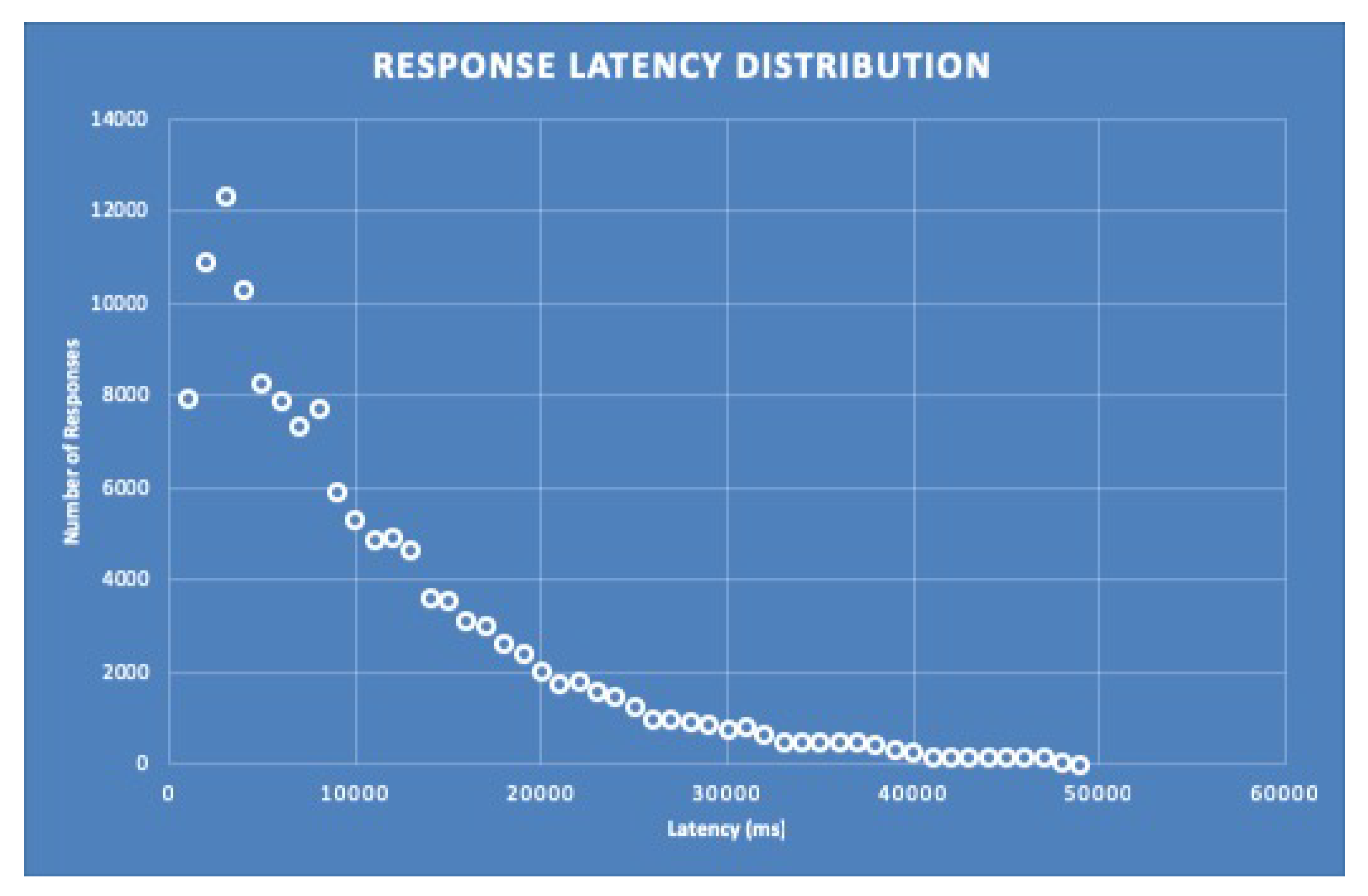
Table 8 we obtain the Pareto-like distribution of the response latency depicted in
Figure 9.
Recall that, as detailed in
Table 8, our simulation scenario assumes fabrication requests with a 5 MB attachment (since this is the typical image file size of a design submitted for fabrication). In addition, we have also assumed that the users (and hence the service requests) are evenly distributed among all the Data centers that form the NEWTON Fab Lab cloud infrastructure.
Table 9 represents the percentiles for the distribution in
Figure 9.
The figure shows the simulation results for the set-up described in
Section 3.11, the configurations reported in
Table 8 and a deployment over 4 AWS regions and represents a simple histogram that groups the system responses with the same delay. In addition,
Figure 9 also demonstrates that the simulator behaves as expected since it matches with very good approximation a Pareto distribution.
The experimental results depicted in
Figure 9 are represented in tabular form in
Table 9.
Observe that 50% of the requests are served within 8.000 ms and 99% of the requests within 38,000 ms, being 49,000 ms the worst case simulated delay. These are indeed excellent results considering that:
As highlighted earlier in this paper, cloud infrastructure is shared among many customers, leading to very variable delays.
The simulated latency also includes the transmission time of the design file (assumed to be 5 MB) attached to a request (that must go from the client to the spoke or hub node of NEWTON infrastructure and finally to the target Fab Lab).
In the worst-case scenario the communication delay depends on the following path: Client–spoke–hub–spoke–Fab Lab–spoke–client. Thus, the latency of a response can be very high due to the communication overhead introduced by each node in the communication path.
Observing the simulation results we can easily infer that the cloud system infrastructure behaves as expected since:
The response delay increases with the number of requests.
The Europe Data center is the one that exhibits the longest delays because it is the hub of our infrastructure and must always process all the incoming requests.
The Data center latency exhibits a high variability, which reflects the performance fluctuations of the cloud infrastructure due to resource and network sharing with other customers as outlined previously.
The response latency exhibits a Pareto-like distribution, which is typical of internet networked systems.
5. Discussion
FaaS Fab Lab deployment has been performed as part of the NEWTON platform. The platform is now in production phase and includes the Cloud Hub (deployed on an Amazon AWS EC2 cluster) and the on-premises interface infrastructure (implemented with inexpensive Raspberry Pi III boards) that has been deployed and is presently under test at CEU Madrid, Spain. This deployment has helped gaining significant insights on several design and implementation aspects and trade-offs that include hardware design and interfacing, system monitoring and cloud deployment, data security as well as service deployment and orchestration in a multi-cloud environment. Several architectural aspects and implementations have been evaluated and tested so far, with particular emphasis on:
system replicability and scalability;
system costs and maintainability;
service availability and auto-discovery in multi-cloud environments;
API architecture and design;
functional and load tests design.
The next step is setting-up the system staging environment that involves networking and interfacing to the cloud hub the Fab Labs at CEU Madrid and Vrije University of Bruxelles, Belgium. This will enable testing the system in a distributed, yet still controlled environment.
FaaS enhances existing Fab Lab capabilities by providing the digital fabrication equipment with the possibility to communicate over the Internet in order to remotely control fabrication activities. Using this approach, the fabrication facilities are exposed to the Internet as software services, which may be consumed by third-party applications.
As described in [
11], FaaS practical deployment strongly relies on IoT and Cloud architectural and software paradigms and requires design and development of specific hardware and software interfaces that allow pervasive connectivity. More specifically, a standard fabrication machine is enhanced by wrapping it with software interfaces running on an external inexpensive microcontroller that acts as the machine ”master”. These interfaces provide a software abstraction layer that enable communication through lightweight machine-to-machine protocols, machine status monitor through current sensors that allow to detect the machine status (either busy, idle or off-line) by measuring the current consumption and machine virtualization through REST APIs. A Fab Lab gateway provides an access point to the machines of a Fab Lab and implements security and rate limiting policies to ensure a fair access to the fabrication resources.
The hardware interface design was not difficult and has been accomplished by using standard and inexpensive off-the-shelf components. Conversely, firmware and software development was highly challenging and has involved solving several complex problems related to equipment monitoring and real time communications. A minimum cloud deployment on one AWS region and with just one container allocated to the application was load tested for different workloads and the results are reported in
Table 10.
Table 10 depicts the APIs response time when the system is loaded by 50, 100 and 150 concurrent users, respectively. Observe that the distribution of the measured delays has “tail” behaviour with a large variability between the minimum (namely, 137 ms) and the maximum (namely, 9141 ms) measured value. The outputs of our simulator, reported in
Section 4, exactly match this “tail” behaviour. As highlighted before, this large variability of the response times is due to the fact that many cloud customers are sharing the same hardware and network infrastructure, which makes a cloud application very sensitive to other users’ workloads. Despite the intrinsic shortcomings of the cloud infrastructure, the measured response times are excellent. Our simulator allows the estimation of system performance at a larger scale, increasing considerably the number of concurrent users and considering a more complex deployment over several AWS regions. Simulation results are summarized in in
Section 4: The response times exhibit Pareto distribution and a high variability ranging from few hundred ms to 49,000 ms (however, 99% of the requests are served within 38,000 ms) in the case of 1500 concurrent users.
This paper describes FaaS deployment in the context of NEWTON next generation Fab Labs; however, the proposed solution is general, hardware-independent and targets all those scenarios which involve collaborative fabrications. We foresee that this capability will have a huge impact not only on education, but also on industry helping to develop new business models in which fab-less companies may schedule medium or large-scale fabrication batches hiring third-party remote fabrication services.
NEWTON has been the opportunity for the whole research team to gain particular insight on the impact of the technology on the way we teach and learn. On one hand we had to investigate new teaching techniques and contents to make STEM subject education more appealing for younger generations, on the other, we had to select those technologies that were more suitable to deliver those contents to a wide audience. We think that Fab Labs are a powerful tool to develop informal teaching activities in which the learning process is based on prototyping and experimentation; however, a Fab Lab is expensive and its deployment costs cannot be afforded by all the institutions, especially the primary and secondary schools that are targeted by the NEWTON project. In this context, cloud and IoT technologies have been proven to be very effective to implement resource sharing and remote access to distributed fabrication equipment. NEWTON has entailed several challenging tasks for us both as engineers and as educators due to the the broad and interdisciplinary nature of the project. However, the whole process from design to development and deployment in production has been productive and enriching and has allowed us to get a better understanding on several cutting-edge technologies (cloud infrastructure architecture and design patterns, IoT technologies, distributed and real time programming, simulation, etc.) and how to integrate them into a working platform that has been battle-tested in several pilot tests. However, the technology developed within NEWTON project it is not an end in itself, but serves a well defined purpose: To foster passion for STEM education through younger generation through the development of innovative technology-enhanced teaching techniques. Under this point of view, the results obtained so far are very encouraging. The test pilots we carried out [
8,
9,
10] showed a high degree of satisfaction among the surveyed students which encourages us to follow this path in our future research.
6. Conclusions
In this work we have introduced the concept of Fabrication as a Service (FaaS) in the context of NEWTON Fab Labs. While, as stated earlier, this concept is broad and general and has many potential applications in several different areas, we have analyzed its impact in education by implementing a resource sharing mechanism that enables remote access and monitoring of expensive digital fabrication equipment. The impact of this technology on the learning outcomes and students’ satisfaction has been assessed through many test pilots whose results have been reported in [
8,
9,
10]. The proposed architecture relies on a complex distributed containerized infrastructure of loosely coupled microservices running both on the cloud an on the Fab Lab premises. The design, deployment and testing of this infrastructure has been thoroughly described in [
11]. More specifically, [
11] targets several important aspects of the platform design including: The design of the fabrication machine hardware wrappers and interfacing, the architecture of the software wrappers and of the cloud-deployed services, the implementation of the security policies and of the communication protocols and the load test of the platform under several load conditions. The tests performed in [
11] helped us to gain more insight on platform behaviour and performance; however, they where carried out only for the deployment that is presently in production and don’t provide information on system performance as it scales over a wider geographical area to interconnect a larger number of Fab Labs. To overcome this limitation we have used the measured data to build a simulation model that allows to estimate system performance under a wide number of configuration and loads. A platform simulator tool is of paramount importance not only to evaluate system performance in a variety of possible scenarios, but also to make the correct design decisions, to detect possible bottlenecks and to allocate the suitable number of cloud resources to cope with users’ demand and target Quality of Service (QoS). In this work we have presented the algorithms we have used to build a simulator of the NEWTON Fab Lab platform. More specifically we have: Introduced the architecture of the hardware and software infrastructure of the NEWTON Fab Lab platform, discussed the modelling challenges and issues of cloud infrastructure, built a simple mathematical model based on multiple linear regression on the measured data, described the simulator architecture and defined a set of experiments to estimate system performance over a wide cloud deployment covering several Amazon AWS regions. The behaviour of the simulated outputs matches exactly the behaviour of the real system; however, our simulator allows the possibility to analyze and evaluate the performance of complex deployments under a broad range of system loads, detecting possible system bottlenecks and architectural flaws.
Cloud, containerization and IoT technologies are enabling a wide range of new applications and business models. FaaS strongly relies on those technologies to implement a novel distributed Fab Labs architecture in which the underlying hardware is wrapped by a software service accessible through APIs. Distributed systems have been around for decades; however, the main driver for the transition from monolithic to loosely coupled distributed architectures has been the widespread and rapid acceptance of the new containerization technologies. Container technologies have allowed the development and rapid deployment of new stacked distributed design patterns [
18,
19] in which the underlying IT infrastructure is clearly decoupled from the application. More specifically, quoting Brendan Burns’ words [
20]:
“From the beginning of the container revolution two things have become clear: First, the decoupling of the layers in the technology stack are producing a clean, principled layering of concepts with clear contracts, ownership and responsibility. Second, the introduction of these layers has enabled developers to focus their attention exclusively on the thing that matters to them — the application.”
In the specific case of the NEWTON Fab Lab platform presented in this paper, containerization and cloud technologies have enabled the possibility to deploy a set of loosely coupled microservices that allow seamless communication and interaction of digital fabrication services. On the other hand, IoT technologies provide the possibility to wrap the underlying digital fabrication hardware with a software abstraction layer transforming a conventional machine into a smart object with the capability to interact with other objects of the NEWTON infrastructure through a cloud hub and machine-to-machine communication protocols.


