Unbalanced Web Phishing Classification through Deep Reinforcement Learning

Abstract

Web phishing is a form of cybercrime aimed at tricking people into visiting malicious URLs to exfiltrate sensitive data. Since the structure of a malicious URL evolves over time, phishing detection mechanisms that can adapt to such variations are paramount. Furthermore, web phishing detection is an unbalanced classification task, as legitimate URLs outnumber malicious ones in real-life cases. Deep learning (DL) has emerged as a promising technique to minimize concept drift to enhance web phishing detection. Deep reinforcement learning (DRL) combines DL with reinforcement learning (RL); that is, a sequential decision-making paradigm in which the problem to be addressed is expressed as a Markov decision process (MDP). Recent studies have proposed an ad hoc MDP formulation to tackle unbalanced classification tasks called the imbalanced classification Markov decision process (ICMDP). In this paper, we exploit the ICMDP to present a double deep Q-Network (DDQN)-based classifier to address the unbalanced web phishing classification problem. The proposed algorithm is evaluated on a Mendeley web phishing dataset, from which three different data imbalance scenarios are generated. Despite a significant training time, it results in better geometric mean, index of balanced accuracy, F1 score, and area under the ROC curve than other DL-based classifiers combined with data-level sampling techniques in all test cases.

1. Introduction

Despite the proliferation of alternative communication tools, such as electronic messages, mobile applications, and social media channels, email remains a popular communication method. As business-critical email volumes grow, the need for automated malicious email recognition tools, such as phishing email detectors and filters, increases. The aim of phishing is to fool users by posing as other subjects to steal confidential data. The concept drift identifies non-predictable and frequent time-dependent evolution of some streams of data, resulting in the absence of stationary data models [1]. This is a common scenario for web data [2], such as phishing URLs, since these are often ephemeral. Therefore, the detection techniques that are now effective may no longer be suitable in the future. machine learning (ML) has proven to be beneficial in addressing the phishing URL classification problem, since an ML-based system is able to generalize, minimizing concept drift, as observed in [3]. As a subfield of ML, deep learning (DL) involves algorithms inspired by the structure and functions of the human brain, the so-called deep neural network (DNNs). deep reinforcement learning (DRL) belongs to the DL field, since DNNs are used as estimators of the functions involved in complex reinforcement learning (RL) problems [4]. In the RL paradigm, an agent interacts with an environment in discrete time steps so that t denotes a single step, following a trial-and-error strategy. Such interactions assume that the task to be addressed can be modeled as a Markov decision process (MDP), described by the tuple $\langle S,A,\Phi ,f_R,\zeta \rangle$, where: S represents the observation space; A is the action space; $\Phi$ is a state-transition function $\Phi :S\times A\times S\to [0,1]$, which describes the probability of observing a state $s_t$, taking action $a_t$ and producing a new state $s_{t+1}$; $f_R$ is the so-called reward function, defined in each t as $R_t$ = $f_R(s_t,a_t)$; $0\le \zeta <1$ is the discount factor, which balances the contribution of immediate and future rewards. During the training phase, the agent learns a policy $\pi$, allowing it to select the next action according to a probability function ${\mathcal{P}}_e$, i.e., $\pi :S\to A$. The goal of all RL agents is to find an optimal policy ${\pi }^{*}$ that maximizes the expected cumulative discounted reward, i.e., long-term rewards [5]. The deep Q-network (DQN) [6] is a classical DRL algorithm that addresses the RL problem by employing two DNNs and a replay buffer to make learning more stable in the case of a large $S\times A$ space. However, it suffers from overestimation [7], which causes maximization bias during learning. To reduce this phenomenon, the double deep Q-network (DDQN) was introduced in [8].

Recent studies focus on the application of DRL algorithms, such as DQN or DDQN, to detect sophisticated cyberthreats, emphasizing the promising results obtained [9,10,11]. This motivated Quang Do et al. [12] to include a DRL framework in their systematic literature review on the use of DL for web phishing detection. However, the list of algorithms belonging to this field appears to be limited only to the contribution proposed in [13], which is a DQN-based classifier. The benchmark analysis proposed in [9] shows that DDQN can perform better than DQN over different cyberthreat detection tasks. Furthermore, the web phishing classification problem is unbalanced, since in real-life cases, the number of legitimate URLs is far greater than the malicious ones [14]. The adoption of data-level approaches represents one of the main strategies for handling data imbalance [15]. These employ undersampling or oversampling algorithms to adjust the sample distribution within different classes. However, an undersampling technique could remove relevant instances from the majority class if it is randomly performed [16]. On the other hand, oversampling techniques increase data complexity, requiring a longer training time [17] for a DL algorithm, which increases with the effective model complexity, since it is influenced by data complexity [18]. According to [12], a long training time is a current limitation of DL models when applied to web phishing detection problems; therefore, the usage of techniques that result in increased training time must be avoided. Several data sampling algorithms have been employed to deal with class imbalance in web phishing classification [19,20]. In some cases, hybrid techniques, which combine both under- and oversampling methods, have been explored to handle unbalanced classes in web phishing datasets [21]. However, although mitigated, the aforementioned disadvantages remain.

This paper presents a DDQN-based classifier to address the web phishing detection task without using prior data-level balancing techniques. The proposed contribution is a cost-sensitive approach that takes advantage of the MDP formulation presented in [22], called the imbalanced classification Markov decision process (ICMDP). In this formulation, the reward function embeds the data balancing ratio, defined as the ratio between the number of malicious and legitimate URLs. In such a way, the learner can distinguish the sample distribution within classes according to the absolute reward value in response to a classification action. In particular, the (in)correct classification will be (less) more rewarded, with an absolute value that will be higher for minority and lower for majority class recognition, respectively.

The contribution provided by this paper is three-fold:

• It extends the current state-of-the-art in DRL algorithms that addresses the web phishing detection task.
• It extends the algorithm proposed in [13] since:
  • The ICMDP formulation is used to tackle class skew in web phishing detection;
  • DQN is replaced with DDQN.
• It shows a benchmark between the proposed DDQN-based classifier and some state-of-the-art DL algorithms combined with data-level sampling techniques, in which metric scores suitable for unbalanced classification problems and algorithm timing performance are evaluated.

The remainder of this paper is organized as follows. Section 2 provides some DRL theoretical framework and a literature review on: (i) the use of DRL for intrusion-detection purposes; (ii) the approaches for dealing with the unbalanced web phishing classification task. Section 3 describes the proposed DRL-based classifier. Section 4 shows the experimental settings, that is, the description of the methods and materials used in this paper. Section 5 illustrates the experimental results and their critical evaluations. Lastly, conclusions with the main findings and insights are reported in Section 6.

2. Background and Related Work

2.1. Reinforcement Learning

Reinforcement learning (RL) agents are generally trained in episodes, each consisting of a certain number of steps. Given an episode, the sequence of states, actions, and rewards builds the trajectory or rollout of $\pi$. Let k be the index assigned to an episode; the cumulative discounted reward is defined as $C_R={\sum }_{k=0}^{\infty }{\zeta }^k{R}_{t+k+1}$. Then, the objective function to be optimized can be indicated as $Q(s_t,a_t)={\mathbb{E}}_{\pi }\left[C_R\right|s_t=s,a_t=a]$, and the maximization problem, which the agent tries to solve, aims at finding $Q^{*}(s_t,a_t)={max}_{\pi }Q(s_t,a_t)$ for all $s\in S$ and $a\in A$ [5].

Q-Learning

One of the most popular RL algorithms, belonging to the class of tabular ones, is Q-learning [23]. It is based on a lookup table (Q-table) that stores the expected rewards (Q-values) for actions with respect to each state in the environment. The Q-value update function for state-action pairs, as expressed in [23], is the following:

$$Q(s_t,a_t)\leftarrow Q(s_t,a_t)(1-\alpha )+\alpha [R_{t+1}+\zeta \underset{a\in A}{max}Q(s_{t+1},a)]$$

(1)

where $0<\alpha \le 1$ represents the learning rate, which determines how the new value influences the older one. However, in some applications, billions of possible unique states and several available actions are required. In such a context, the Q-table requires a large amount of memory to be stored. Therefore, Q-learning becomes unreliable in practice [4]. To solve such a problem, DNNs have been adopted to approximate the function occurring in RL problems, thus providing the opportunity to introduce deep reinforcement learning (DRL).

2.2. Deep Reinforcement Learning

2.2.1. Deep Q-Network

Whenever the $S\times A$ space is very large, it will be impractical to evaluate Q-values in closed form, hence function approximations are used. For example, the deep Q-network (DQN) [6] employs a DNN such that $Q^{*}(s_t,a_t)\approx Q(s_t,a_t,\theta )$, where $\theta$ represents a vector containing DNN parameters. This network, called Q-network, takes the current state and action as inputs and estimates the Q-value. Furthermore, Mnih et al. [6] proposed two original contributions: (1) the target network $\widehat{Q}$ and (2) the experience replay. $\widehat{Q}$-network is used for the target value estimation:

$$y_t^{DQN}=R_{t+1}+\zeta \underset{a\in A}{max}\widehat{Q}(s_{t+1},a,{\theta }^{-})$$

(2)

where ${\theta }^{-}$ represents the $\widehat{Q}$-network parameters. This calculation is not dependent on the Q-function estimation, since $\widehat{Q}$-network shares Q-network model size, but in every $\tau$ step, the operation ${\theta }^{-}\leftarrow \theta$ is performed. Experience replay uses a first-in first-out (FIFO) queue, called replay buffer $\mathcal{B}$, to store an experience tuple $e_t=\langle s_t,a_t,s_{t+1},f_R(s_t,a_t),{\sigma }_t\rangle$ for each t, where the binary indicator ${\sigma }_t$ determines whether $s_t$ is a terminal state. In such a way, during the training phase, to reduce correlations due to the sequencing of observations, a mini-batch b of experience tuples is selected according to the probability function ${\mathcal{P}}_s$ from $\mathcal{B}$. Therefore, b is used to update $\theta$, using a gradient descent algorithm to minimize a differentiable loss function, which in the case of DQN has the form:

$${\mathcal{L}}^{DQN}\left(\theta \right)=\mathbb{E}\left[{(y_t^{DQN}-Q(s_t,a_t,\theta ))}^2\right]$$

(3)

In (2), the max operator selects and evaluates actions using the same values. Thus, it is more likely that these values will be overestimated, i.e., will be chosen every time the action that results in the highest Q-value for a particular state. This phenomenon, known as overestimation, affects DQN [7] and introduces a maximization bias in learning, causing a slowdown in convergence. To reduce such a bias, H. van Haselt et al. [8] introduced the double deep Q-network (DDQN).

2.2.2. Double Deep Q-Network

The double deep Q-network (DDQN) separates action selection and action evaluation processes according to the theoretical basis behind the original DQN algorithm [24]. Rather than using the update function expressed by Equation (1), the DDQN strategy is based on the update functions shown in [23]:

$$Q^{\left(1\right)}(s_t,a_t)\leftarrow Q^{\left(1\right)}(s_t,a_t)(1-\alpha )+\alpha [R_{t+1}+\zeta \underset{a\in A}{max}{Q}^{\left(2\right)}(s_{t+1},a)]$$

(4)

$$Q^{\left(2\right)}(s_t,a_t)\leftarrow Q^{\left(2\right)}(s_t,a_t)(1-\alpha )+\alpha [R_{t+1}+\zeta \underset{a\in A}{max}{Q}^{\left(1\right)}(s_{t+1},a)]$$

(5)

A Q-function ($Q^{\left(1\right)}$) changes its value according to the value of another Q-function ($Q^{\left(2\right)}$), and both value functions determine the action. DDQN does not add any new network compared to DQN, since the $\widehat{Q}$-network is a natural candidate to approximate the second Q-function [5]. In this case, the target value is calculated as follows:

$$y_t^{DDQN}=R_{t+1}+\zeta \widehat{Q}(s_{t+1},\underset{a\in A}{arg\; max}Q(s_{t+1},a,\theta ),{\theta }^{-})$$

(6)

Therefore, the Q-network selects the action $a_t$ that results in the maximum Q-value of the next state, and the target network computes the estimated Q-value according to the action $a_t$ previously selected. The usage of $\mathcal{B}$ introduced in DQN is still valid. As a consequence, during the learning process, a mini-batch $b\in \mathcal{B}$ is used for updating the main network parameters, minimizing a differentiable loss function, which in the case of DDQN has the form:

$${\mathcal{L}}^{DDQN}\left(\theta \right)=\mathbb{E}\left[{(y_t^{DDQN}-Q(s_t,a_t,\theta ))}^2\right]$$

(7)

The $y_t^{DDQN}$ steps, which are different from those of $y_t^{DQN}$, can be summarized as follows: Q-network uses the next state $s_{t+1}$ to calculate $Q(s_{t+1},a)$ for each possible action in A that can occur in $s_{t+1}$. Thus, the action selection process is implemented by the operation ${arg\; max}_{a\in A}$ applied in $Q(s_{t+1},a)$, which selects the best action $a^{*}$ resulting in the highest Q-value. Finally, the action evaluation process is performed using the $Q(s_{t+1},a^{*})$ value (evaluated by using the $\widehat{Q}$-network) that belongs to the action $a^{*}$ (selected by using the Q-network) to compute $y_t^{DDQN}$. Note that target value formulas such as (2) and (6), in the case of a terminal state, i.e., ${\sigma }_t=1$, assume a value equal to the current reward $R_t$.

2.3. Deep Reinforcement Learning for Intrusion Detection

According to [25], current and future research directions should converge toward the exploration of DRL techniques for intrusion-detection purposes. T.T. Nguyen et al. [10] evaluated the increased usage of DRL to solve complex cybersecurity problems in different application fields such as cyberphysical systems security, game theory for attacking purposes, and intrusion-detection systems. In [11], a review of the applications of DL-based algorithms in the cybersecurity domain is provided, listing several DRL-based algorithms used for different cybersecurity purposes, such as intrusion and/or malware detection/prevention. An extended review of several DRL algorithm applications in the cybersecurity field is provided in [26], focusing on DRL applications for Internet of things (IoT) and modern networks protection; adversarial attacks on existing ML classifier generation; network intrusion detection and prevention as a binary classification task.

In this regard, the usage of DRL for intrusion-detection purposes is analyzed in [9]. In particular, it takes into account four DRL algorithms, such as DQN, DDQN, policy gradient (PG), and actor critic, and compares them with several ML algorithms on NSL-KDD and AWID datasets. The obtained classification scores show that DDQN outperforms the other DRL-based algorithms. In addition, the resulting scores are comparable to those achieved by support vector machine (SVM) in NSL-KDD and shallow learning algorithms in AWID.

In [27], Y. Liu et al. proposed a deep deterministic policy gradient (DDPG) algorithm for denial of service (DoS) and distributed denial of service (DDoS) flooding attack mitigation on software-defined networks (SDNs). The proposed DDPG has been compared with common router-throttling methods in a simulated environment, resulting in a better mitigation effect against DDoS attack.

In [28], the authors address the network intrusion-detection problem through a multi-agent collaborative reinforcement learning framework, called Major-Minor-RL. It is based on a DDQN agent combined with several minor agents that support the decision-making process of the major agent using a different observation space. This framework has been evaluated on the NSL-KDD dataset, resulting in very promising classification performances compared to those achieved by traditional ML and DL algorithms.

In [29], the network intrusion-detection task is tackled using a semi-supervised version of the DDQN algorithm. In particular, DDQN is combined with two unsupervised learning algorithms, i.e., autoencoder (AE) and K-means. The method, called SSDDQN, has been evaluated on the NSL-KDD and AWID datasets, resulting in good classification metric scores.

In [30], the authors present a DQN-based intrusion-detection system, where the agent is rewarded positively or negatively for correctly predicting intrusions. Such an approach has been evaluated using the UNSW-NB15 and NSL-KDD datasets. A preliminary analysis was performed to correctly tune the agent hyperparameters; then, the optimized DQN was compared with several ML and DL algorithms, achieving better classification performances. The same datasets are used by Y.F. Hsu in [31], where a DQN-based intrusion-detection system is proposed in combination with peculiar pre-processing and feature selection strategies. The DNNs used in DQN are tuned according to the results provided by the Adadelta optimizer. This approach has been compared with different ML algorithms such as SVM, multi-layer perceptron (MLP), and random forest (RF). The results obtained show that DQN achieves better accuracy and precision scores than other classifiers.

In [32], a DQN-based classifier has been evaluated on the NSL-KDD dataset, obtaining better true positive rate results than baseline classifiers, such as RF, MLP, and SVM. As a consequence, the DQN-based solution results in a better dependability property.

Caminero G. et al. [33] used DQN both as an environment and as an agent classifier to propose the so-called adversarial environment RL (AE-RL). The first agent selects the sample, i.e., the observation that will be used during the next training step, while the second one classifies the current observation. AE-RL has been tested on NSL-KDD and AWID datasets, outperforming the compared classifiers.

In [34], the DQN is combined with a convolutional neural network (CNN) to realize a novel network intrusion-detection framework at the packet level. One of two different kinds of CNN is used as a feature learning layer to transform network packets into images; then, the output is passed to the DQN classifier that estimates Q-values to compare with an anomaly threshold. The combination between CNN and DQN outperforms RF, SVM, Adaboost, CNN, and the combination between CNN and PG, among the tests performed using the CICDDoS2019 dataset.

Alavizadeh H. et al. [35] use a DQN-based classifier for network intrusion-detection purposes, using hyperparameters optimally tuned to enhance agent learning capabilities. In this way, the agent can effectively classify anomaly packets within NSL-KDD, achieving a better accuracy score than the self-organizing map (SOM), SVM, Naïve Bayes SVM, RF, and bidirectional long short-term memory (BiLSTM) classifiers.

To the best of our knowledge, the only implementation of a DRL-based classifier for web phishing detection is the one proposed by M. Chatterjee and A.S. Namin [13]. In particular, a DQN-based classifier is used, such that the agent is encouraged to recognize malicious URLs by the effect of a greater reward as a consequence of a correct classification. Otherwise, a null reward is received by the agent. The DQN-based web phishing detector has been evaluated using the Ebbu2017 Phishing dataset, achieving promising classification metric scores. However, in [13], the data imbalance has not been taken into account since the agent is rewarded independently of the class to which the observed sample belongs. Furthermore, according to [9], a DDQN has to be explored for network intrusion-detection scopes, such as the one addressed in our work.

2.4. Handle Class Imbalance in Web Phishing Classification

Several cybersecurity problems suffer from class imbalance. In [36], the authors analyzed different sampling algorithms to tackle class imbalance in cybersecurity datasets. Bootstrap aggregation (BAGGING), synthetic minority oversampling technique (SMOTE), random undersampling (RUS), and class balancer were analyzed. These were combined with several ML classifiers and address the class imbalance present in the UNSW-NB15 dataset. The synthetic minority oversampling technique (SMOTE) results in better average performances than other sampling techniques.

The investigation proposed in [37] extends the analysis using other techniques such as adaptive synthetic (ADASYN), Tomek-Link (T-Link), and T-Link with ADASYN combined with DL models, such as MLP, CNN, and a combination between a CNN and a particular type of recurrent neural network (RNN), that is, a BiLSTM. Furthermore, the evaluation of sampling techniques is extended, considering the combination between random undersampling (RUS) and random oversampling (ROS). This analysis is performed using the NSL-KDD dataset. The results show that the proposed CNN, combined with the aforementioned data-level sampling techniques, performs better in binary classification tasks, while in multiclass problems, MLP achieves better performances than other DL models.

Web phishing classification is one of the main cybersecurity problems suffering from data imbalance [14]. Several ML classifiers, such as decision tree (C5.0), SVM and naïve Bayes have been evaluated in different imbalance data scenarios in [38]. Each of them is obtained by varying the imbalance factor, defined as the ratio between the number of samples within the minority class with respect to the number of samples within the majority class. The proposed investigation regards the evaluation of the area under receiving operating characteristic (AUC) for different imbalance ratio values. The results show that the compared classifiers achieved higher AUC when the imbalance ratio is equal to $0.25$ for C.50 and naïve Bayes.

In [20], three different data-level techniques are used, i.e., RUS, ROS, and SMOTE, combined with several ML algorithms, to conduct an extended comparison on unbalanced web phishing classification. The evaluated classifiers are: (i) logistic regression, (ii) SVM, (iii) decision tree, (iv) RF, and (v) stochastic gradient descent (SGD). The benchmark performed on the Kaggle website dataset shows that RF outperforms the other classifiers when combined with ROS.

In [39], the unbalanced dataset is divided into phishing and legitimate categories. Then, the training dataset is obtained using 90% of the phishing samples and the same quantity of legitimate samples. In particular, the number of samples within the majority class is reduced using the RUS technique. The remaining data are used as a test set for evaluating RF, SVM, logistic regression, naïve Bayes, and Adaboost. Among the classifiers compared, RF achieved the best accuracy and detection rate values.

In [40], a semi-automated feature generation for phishing classification (SAF${}_E$-PC), which is a classifier based on ensemble learning capable of handling the unbalanced nature of web phishing, is proposed. In particular, the classifier used is a RUS-Boost algorithm, which is preferred to a SMOTE-Boost, since the adoption of SMOTE results in a higher number of training samples and, consequently, in a higher training time. Furthermore, SMOTE is more computationally expansive than RUS, which handles data imbalance randomly.

In [19], the authors address the web phishing classification task employing Salp Swarm and Emperor Penguin metaheuristic optimization algorithms to tune a DNN classifier. This approach has been evaluated using the Mendeley web phishing dataset, which is initially processed to reduce the number of features, and the data imbalance level through principal component analysis (PCA) and SMOTE, respectively. Performance evaluation focuses on reducing training time with respect to a neural network that does not employ any hyperparameter optimization. The classification performance has been evaluated using the accuracy metric, which is the same for all approaches compared.

In [41], the SMOTE technique is used to adjust the distribution of data within the UCI web phishing dataset, resulting in an overall improvement in classification performance for SVM, RF, and XGBoost.

S. Priya et al. [42] combined ADASYN with an Adadelta optimizer-based DNN to present a DL-based algorithm for handling the concept drift due to data imbalances in web phishing classification tasks. The algorithm has been evaluated on three different datasets, showing better performance as a web phishing classifier than several ML models, such as K-nearest neighbor (K-NN), naïve Bayes, etc.

In [21], SMOTE as an oversampler and one-sided selection (OSS) as an undersampler and their combination as a hybrid technique are employed to handle data imbalances in web phishing classification. The dataset used is the UCI Websites, and the algorithms evaluated are SVM, MLP, decision tree (C4.5), and K-NN. MLP combined with OSS-SMOTE achieves the best accuracy and geometric mean scores.

In [43], SMOTE is applied to address the UCI dataset class skew. Then, several classifiers were evaluated using both balanced and unbalanced dataset versions. As a result of the SMOTE application, a marginal improvement was observed for some algorithms.

In [44], a cost-sensitive variant of XGBoost is presented to address the unbalanced classification problem of malicious URLs. This is realized by introducing a cost-sensitive factor into the classifier loss function to weight misclassification cases. Such an approach has been compared with the classical XGBoost and with the XGBoost combined with SMOTE, resulting in better problem-specific metric scores. A novel approach to detect malicious URLs, mitigating the concept drift, is presented in [45]. In this case, the class imbalance is tackled using the RUS technique.

In [46], the problem of class imbalance is addressed through a two-module framework. The so-called combining module is delegated to tackle the class skew as it embeds a cost-sensitive DNN metaclassifier. This framework has been compared with CART and ensemble learning methods, resulting in a better F1 score for different class imbalance ratio values.

In [47], a novel malicious URLs detector, based on a combination of a deep AE (DAE) and a CNN, is presented. First, the DAE defines the URL template, considering only legitimate URLs to cope with the class imbalance. According to such a template, an abnormal score is defined, and then, the CNN uses it to improve the phishing URLs detection rate. This approach has been evaluated using three different datasets with different values of balancing ratio, resulting in promising classification scores.

In [48], the imbalance data problem is addressed using a generative adversarial network (GAN) to synthesize new samples for the minority class. Furthermore, a CNN is combined with a multi-head self-attention mechanism to realize the malicious URLs classifier. In several tests performed, GAN results in better classification metrics compared to those obtained using the SMOTE technique. A GAN is also used in [49] to adjust the distribution of unbalanced malicious URLs. Furthermore, since GAN can create many synthetic samples of the minority class, the K-means algorithm is used to select the most representative.

Naim O. et al. [50] address the identification of malicious websites at page-level design. Therefore, starting from a URL, it is classified as malicious or legitimate according to the features of the website to which it points. Two classification algorithms have been evaluated for such a purpose, i.e., DNN and ensemble learning. The class imbalance is addressed by employing the RUS technique. This strategy has been preferred to the use of data augmentation of samples within the minority class, since the latter results in an active manipulation of the original data distribution. Such an operation alters the accurate representation of a real-life scenario.

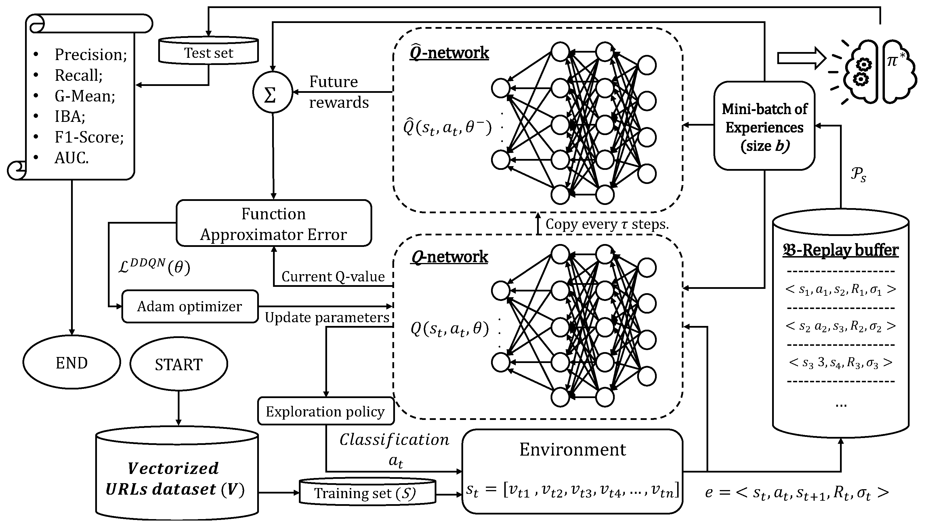
3. Combining ICMDP with DDQN for Unbalanced Web Phishing Classification

To address the problem of detecting phishing websites, this paper proposes a DRL-based classifier. The employed paradigm requires that each URL must be pre-processed to transform the categorical data into a numerical vector. Therefore, given a collection of URLs $\mathcal{U}$, it must be represented as a matrix $V\in {\mathbb{R}}^{\left|\mathcal{U}\right|\times n}$. In particular, a function $f_T:\mathcal{U}\to V$ transforms each $u\in \mathcal{U}$ into an integer vector $v\in V$, composed of n features extracted from the original URL. As a result, the vectorized collection V can be used as an experience by ML algorithms to perform classification tasks.

3.1. ICMDP Environment Setting

To model the RL environment, each element of the MDP tuple is set according to the ICMDP formulation [22] as follows:

• The observation space S is given by the training set, i.e., $S\subset V$. As a consequence, each training sample represents an observation $s_t$ on a given t. In our model, positive samples are the phishing URLs and represent the minority class denoted with $S_P$. On the other hand, the negative class comprises legitimate URLs representing the majority class $S_N$. Hence, $S=S_P\cup S_N$.
• The action space A consists of the set of predictable class labels. In particular, $A=\{0,1\}$, where 0 and 1 are the negative and positive sample labels, respectively. Therefore, $\pi :S\to A$ guides the agent classification actions according to ${\mathcal{P}}_e$.
• The reward function $f_R$ gives feedback on the quality of classification actions performed by the agent during its learning phase. In particular, the agent is positively rewarded if it correctly classifies a sample belonging to $S_P$, i.e., if the action performed results in a true positive (TP). On the contrary, the agent is negatively rewarded if the classification action performed on a sample belonging to $S_N$ results in a false positive (FP). The classification actions related to samples belonging to the majority classes are rewarded based on the actual balancing ratio $\rho =\frac{|S_P|}{|S_N|}\in [0,1]$. In particular, $-\rho$ corresponds to a misclassification of a sample belonging to $S_P$, i.e., a false negative (FN); otherwise, $\rho$ is assigned to a correct classification of a sample belonging to $S_N$, i.e., a true negative (TN). Since $R_t$ of the minority class is higher (in absolute value) than that of the majority class, the agent will be more sensitive in classifying samples belonging to $S_P$. Finally, $R_t$ can be expressed as:

  $$R_t=f_R(s_t,a_t,l_t)=\left\{\begin{array}{cc}\hfill 1,\hfill & \hfill a_t=l_t\mathrm{and}{s}_t\in S_P\hfill \\ \hfill \rho ,\hfill & \hfill a_t=l_t\mathrm{and}{s}_t\in S_N\hfill \\ \hfill -1,\hfill & \hfill a_t\ne l_t\mathrm{and}{s}_t\in S_P\hfill \\ \hfill -\rho ,\hfill & \hfill a_t\ne l_t\mathrm{and}{s}_t\in S_N\hfill \end{array}\right.$$

  (8)

  where $l_t\in \{0,1\}$ refers to the true value of the class to which the observed sample $s_t$ belongs. Furthermore, $\rho =1\iff |S_P|=|S_N|$, and under such a hypothesis, the reward changes in a formulation as well as in the same expression used in [13].
• Following the definition of S, the states-transition probability function $\Phi$ is deterministic, since the agent moves from $s_t$ to $s_{t+1}$ according to the order in which the samples appear in S.

Hence, for each t, the agent analyzes a training sample $s_t$ and then predicts the class to which it belongs. Given $R_t$ in (8), the $C_R$ is maximized if the agent correctly classifies the samples. Finally, a generic training episode ends when one of these two events occurs:

• All the samples within S are classified.
• The agent classification action results in a FP.

Therefore, a training episode has length $\mathcal{N}$, which is $1\le \mathcal{N}\le \left|S\right|$.

3.2. Reward-Sensitive DDQN Training Phase

According to [9], the adoption of a DDQN is proposed in this paper to avoid the overestimation problem that occurs by using a DQN. Thus, the goal of the agent is to achieve an optimal classification policy, say ${\pi }^{*}$, such that:

$${\pi }^{*}\left(a\right|s)=\left\{\begin{array}{cc}\hfill 1,\hfill & \hfill \mathrm{if}a=\underset{a}{arg\; max}{Q}^{*}(s,a)\hfill \\ \hfill 0,\hfill & \hfill \mathrm{otherwise}\hfill \end{array}\right.$$

(9)

As discussed in Section 2.2, this is achieved by optimizing (7), i.e., updating the Q-network parameters by computing the partial derivative as follows:

$$\frac{\partial {\mathcal{L}}^{DDQN}\left({\theta }_k\right)}{\partial {\theta }_k}=-2\times \sum _{e\in \mathcal{B}}(y^{DDQN}-Q(s,a,{\theta }_k))\times \frac{\partial Q(s,a,{\theta }_k)}{\partial {\theta }_k}$$

(10)

It is essential to observe how $R_t$ formulation (8) influences the learning process, as shown in [22]. Therefore, the $y^{DDQN}$ defined in (6) changes as follows:

$$\left\{\begin{array}{cc}\hfill y_P^T=1+(1-{\sigma }_t)\zeta \widehat{Q}(s_{t+1},{arg\; max}_{a\in A}Q(s_{t+1},a)),\hfill & \hfill \mathrm{target}\mathrm{for}\mathrm{TP}\hfill \\ \hfill y_N^T=\rho +(1-{\sigma }_t)\zeta \widehat{Q}(s_{t+1},{arg\; max}_{a\in A}Q(s_{t+1},a)),\hfill & \hfill \mathrm{target}\mathrm{for}\mathrm{TN}\hfill \\ \hfill y_P^F=-1+(1-{\sigma }_t)\zeta \widehat{Q}(s_{t+1},{arg\; max}_{a\in A}Q(s_{t+1},a)),\hfill & \hfill \mathrm{target}\mathrm{for}\mathrm{FP}\hfill \\ \hfill y_N^F=-\rho +(1-{\sigma }_t)\zeta \widehat{Q}(s_{t+1},{arg\; max}_{a\in A}Q(s_{t+1},a)),\hfill & \hfill \mathrm{target}\mathrm{for}\mathrm{FN}\hfill \end{array}\right.$$

(11)

To simplify the notation, an indicator function $I(a_t,l_t)$ is introduced, grouping all target expressions in (11) per class. Furthermore, derivative (10) can be expressed as the sum of the derivatives of the loss functions associated with samples belonging to minority and majority classes, respectively. Therefore, the resulting equation is composed of three terms, namely $T_1$, $T_2$, and $T_3$:

$$\frac{\partial {\mathcal{L}}^{DDQN}\left({\theta }_k\right)}{\partial {\theta }_k}=-2\times (T_1+T_2+T_3)$$

(12)

where:

$$T_1=\sum _{m=1}^{\left|S\right|}((1-{\sigma }_m)\zeta \widehat{Q}(s_{m+1},\underset{a\in A}{arg\; max}Q(s_{m+1},a,{\theta }_{k-1}))-Q(s_m,a_m,{\theta }_k))\times \frac{\partial Q(s_m,a_m,{\theta }_k)}{\partial {\theta }_k}$$

(13)

$$T_2=\sum _{p=1}^{|S_P|}{(-1)}^{1-I(a_p=l_p)}\times \frac{\partial Q(s_p,a_p,{\theta }_k)}{\partial {\theta }_k}$$

(14)

$$T_3=\rho \times \sum _{n=1}^{|S_N|}{(-1)}^{1-I(a_n=l_n)}\times \frac{\partial Q(s_n,a_n,{\theta }_k)}{\partial {\theta }_k}$$

(15)

Here, $T_2=T_3\iff \rho =1$. In the case of an unbalanced problem, $T_3$ does not dominate $T_2$ due to the $\rho$ effect. Thus, introducing $\rho$ into $R_t$ results in minimizing the impact of $T_3$ on ${\mathcal{L}}^{DDQN}\left(\theta \right)$ in the case that samples from the majority class outnumber those of the minority. As a result, the bias due to class skew is avoided.

4. Experimental Setup

This section reports the methods and materials used during the algorithm performance evaluation. First, the selected dataset and metrics are described. Then, the implementation details of the proposed DDQN-based classifier and the benchmark algorithms are discussed.

4.1. Web Phishing Dataset Description

In this paper, the Mendeley dataset [51,52] is used. According to [53], it represents a state-of-the-art dataset for the web phishing detection problem. In addition, it has been selected since it consists of nearly twice as many samples from the majority class as from the minority class. In

Table 1. Mendeley main characteristics.

No. Phishing URLs	No. Legitimate URLs	No. Features
30,647	58,000	111

, the Mendeley dataset main characteristics are reported.

The selected dataset is a collection of vectorized URLs and consists of a set of numerical features, allowing for the implementation of a cross-language model. Furthermore, some lexical features are independent of any particular web application with a very long lifetime, in contrast to malicious URLs that are often ephemeral. In detail, Mendeley features are based on the decomposition of the original URL into four parts: (i) domain, (ii) directory, (iii) file, and (iv) parameters. For each URL segment, a series of numerical or boolean features are taken into account. In particular, some of them are (a) the domain length, (b) the length of URL query, (c) the number of characters in the form of special characters or letters found in the URL, (d) a boolean value to check the existence of HTTPS, etc. Furthermore, there are some statistical features that determine whether the URL is indexed in search engines such as Whois or Google, or that rank the popularity and importance of the web page on the Internet.

In this work, the dataset has been split into training and test sets using a holdout strategy. In particular, $75\%$ is considered training data, and the remaining $25\%$ represents the test data. Then, the samples within $S_P$ are randomly removed to generate two new test cases; thus, three different data imbalance scenarios are obtained as shown in

Table 2. Different test cases for different $\rho$ values.

$|{\mathit{S}}_{\mathit{P}}|$	$|{\mathit{S}}_{\mathit{N}}|$	$\mathit{\rho }$
23,012	43,473	$0.529$
13,012	↑ *	$0.299$
6506	↑	$0.149$

* The symbol ↑ assigns to the current cell the same value of the above one.

.

4.2. Metrics Used to Evaluate Classification Performance

For evaluation purposes, we select some conventional classification metrics, such as precision, recall (or true positive rate) (TPR), F1 score, defined in Equations (16)–(18), and area under the receiver operating characteristic curve (AUC).

$$\mathrm{Precision}=\frac{\mathrm{TP}}{\mathrm{TP}+\mathrm{FP}}$$

(16)

$$\mathrm{TPR}=\frac{\mathrm{TP}}{\mathrm{TP}+\mathrm{FN}}$$

(17)

$$\mathrm{F}1\mathrm{Score}=2\times \frac{\mathrm{TPR}\times \mathrm{Precision}}{\mathrm{TPR}+\mathrm{Precision}}$$

(18)

According to [54], a high AUC value results in a model robust against class imbalance. Furthermore, the F1 score can work well when data are unbalanced since it represents the harmonic mean of precision and TPR. However, since the positive class is the minority one, the class skew can influence both Equations (16) and (17). As a consequence, to better analyze the unbalanced scenario, the evaluation has been extended by considering the following problem-specific metrics.

• Geometric mean: In binary classification problems, the geometric mean (G-Mean) is calculated as the square root of the product between the TPR and the true negative rate (TNR), where $\mathrm{TNR}=\frac{\mathrm{TN}}{\mathrm{TN}+\mathrm{FP}}$. It measures the balance between classification performances in both minority and majority classes in terms of TPR and TNR, respectively. A very high value of TPR (TNR) can be due to a biased classification that cannot handle data imbalance. This scenario will not result in an acceptable G-Mean value.

  $$\mathrm{G}-\mathrm{Mean}=\sqrt{\mathrm{TPR}\times \mathrm{TNR}}$$

  (19)
• Index of balanced accuracy: Introduced in [55], it measures the degree of balance between two scores. This is achieved using the so-called dominance ${\rm Y}$, which is computed as the difference between TPR and TNR. Since $\mathrm{TPR},\mathrm{TNR}\in [0,1]\to {\rm Y}\in [-1,1]$. As a consequence, both rates are balanced if ${\rm Y}$ is close to 0. The correlation of the G-Mean (for simplicity, the authors suggest the use of ${\mathrm{G}-\mathrm{Mean}}^2$) and the ${\rm Y}$ results in a curve, namely balanced accuracy graph (BAG). The index of balanced accuracy (IBA) is defined as the area of the rectangle obtained considering the following series of points in the BAG: $\left\{\right(-1,0),(-1,\mathrm{g}),(\mathrm{a},\mathrm{g}),(\mathrm{a},0\left)\right\}$, where the point $(\mathrm{a},\mathrm{g})$ represents the trade-off between ${\mathrm{G}-\mathrm{Mean}}^2$ and ${\rm Y}$. The highest $IBA$ value corresponds to $(\mathrm{a},\mathrm{g})=(0,1)$. The weighting factor $0\le \gamma \le 1$ is introduced to make the influence of ${\rm Y}$ more stable. In our experiments $\gamma =0.1$, according to the default value of the Imbalanced-learn library [56].

  $$\mathrm{IBA}=(1+\gamma \times {\rm Y})\times {\left(\mathrm{G}-\mathrm{Mean}\right)}^2$$

  (20)

4.3. DDQN-Based Classifier Implementation Details and Hyperparameter Settings

To implement the model, we take advantage of the source code provided in [57], containing a Python 3.8 implementation of a custom environment for the binary classification of unbalanced datasets and a DDQN agent. Figure 1 shows the implementation workflow providing the main function blocks. Furthermore, the following main libraries have been used: (i) Pandas [58] and Numpy [59] to process input data; (ii) OpenAI Gym [60] to implement the ICMDP environment; (iii) Tensorflow [61] to develop the DDQN Agent; (iv) Scikit-learn [62] and Imbalanced-learn [56] to compute metrics.

According to one of the hyperparameter configurations suggested in the original implementation, the discount rate is set to $\zeta =0.1$. The update $\widehat{Q}$-network parameters (${\theta }^{-}\leftarrow \theta$) period $\tau$ consists of 800 steps. From the model size perspective, two hidden layers for each involved DNN (Q and $\widehat{Q}$) are used, with 256 neurons each. Each node is activated by a rectified linear unit (RELU) function. The agent exploration is performed according to the well-known decayed-$ϵ$-greedy, with a decaying period set to ${10}^4$ and ${ϵ}_{min}=0.5$. Furthermore, ${\mathcal{P}}_s$ is given by a random uniform strategy to sample b from $\mathcal{B}$, where for each episode $\left|\mathcal{B}\right|=2\times {10}^3$. The hyperparameters adopted to update the Q-network parameters by minimizing ${\mathcal{L}}^{DDQN}\left(\theta \right)$ are reported in

Table 3. DDQN-based classifier hyperparameter configuration for loss optimization.

No. Training Episodes	Optimizer	$\mathit{\alpha }$ *	b **
${10}^5$	Adam	$2.5\times {10}^{-4}$	128

* $\alpha$ represents the learning rate. ** b represents the size of the mini-batch sampled from the replay buffer $\mathcal{B}$.

.

4.4. Deep Learning Classifiers and Data Sampling Techniques Selected for Benchmark

This section describes each algorithm compared with the DDQN-based classifier. Since the proposed model extends the systematic review on DL for web phishing detection proposed in [12], several DL classifiers for benchmark purposes are selected according to the literature review discussed in Section 2.4. Moreover, these are combined with several data-level sampling techniques.

4.4.1. Deep Learning Classifiers

As shown in the literature, the following DL algorithms have been combined with data-level sampling techniques to address unbalanced classification tasks, such as web phishing detection. Note that to perform a preliminary comparison, the hyperparameters of the selected DL classifiers are set to obtain a reasonable trade-off between short training time and a good G-Mean score. The G-Mean trend, during the training phase, is monitored, since it influences IBA and achieves a score very close to AUC.

• Deep neural network (DNN): This is a conventional feed-forward neural network having two hidden layers with 256 nodes, with each node having a RELU activation function. The data are then forwarded to the classification layer, which has a unique node with a sigmoid activation function.
• Convolutional neural network (CNN): This model combines convolutional and pooling layers. The first aims at detecting local conjunctions between features, while the second tries to merge semantically similar features into a single one. Therefore, the convolutional layer extracts the relevant features, and the pooling layer reduces their dimensions. Finally, a fully connected layer is used to perform the classification. Datasets that present one-dimensional data, i.e., vector structure, can be processed using a one-dimensional CNN (CONV1D) [63] layer. In particular, the model employs a CONV1D layer with 128 filters, 3 as the kernel size, and a hyperbolic tangent activation function. The data are then forwarded through a flatten layer to a classification node that has a sigmoid activation function.
• Long short-term memory: This is a model belonging to the class of RNN. Unlike a classical feed-forward neural network, an RNN can create cycles. The architecture of long short-term memory (LSTM) introduced in [64] consists of three gates in its hidden layers, namely an input gate, an output gate, and a forget gate. These entities form the so-called cell, which controls the information flow necessary for prediction purposes. The LSTM used in our experiments has 128 units (size of hidden cells) connected to a final layer, which is a classification layer having a sigmoid activation function.
• Bidirectional long short-term memory (BiLSTM): This differs from the above mentioned for the adoption of a bidirectional layer, which can improve prediction accuracy by pulling future data in addition to the previous data captured as input [65].

Finally,

Table 4. Configuration of benchmark algorithm hyperparameters for loss optimization.

Algorithm	No. Training Epochs	Optimizer	$\mathit{\alpha }$ *	Batch Size
DNN	100	Adam	${10}^{-4}$	512
CNN	40	↑ **	↑	256
LSTM	20	↑	$5\times {10}^{-4}$	128
BiLSTM	↑	↑	↑	↑

* $\alpha$ represents the learning rate. ** The symbol ↑ assigns to the current cell the same value of the above one.

shows the hyperparameters involved for loss optimization purposes.

For the sake of clarity, DL models can achieve optimal performance through optimal hyperparameter tuning, as can be seen in [14]. Since this work is focused on a preliminary comparison, rigorous hyperparameter optimization for both the DDQN-based classifier and all the compared algorithms is out-of-scope.

4.4.2. Data Sampling Techniques

The selected data-level balancing strategies are:

• Oversampling:

  –

  Random oversampling (ROS): This technique is the simplest since it randomly duplicates samples within $S_P$ to obtain $|S_P|=|S_N|$.

  –

  Synthetic minority oversampling technique (SMOTE) [66]: This balancing technique initially finds the K-NNs for each sample x within $S_P$ by computing the Euclidean distance between it and all other samples in $S_P$. Then, according to the actual $\rho$ value, a sampling rate $\lambda$ is established, and for each sample in $S_P$, $\lambda$ elements are randomly selected from its K-NNs, to build a new set $S_{P_{{\lambda }_1}}$, such that $|S_{P_{{\lambda }_1}}|=\lambda$. Finally, a new synthetic sample is created for each sample $x_j\in S_{P_{{\lambda }_1}}$, with $j=1,...,\lambda$, using the following formula: $x_{NEW}=x+f_{RAND}(0,1)\times |x-x_j|$, where the function $f_{RAND}(0,1)$ randomly selects a number between 0 and 1.

  –

  Adaptive synthetic (ADASYN) [67]: This strategy initially computes $\rho$ and the number of synthetic data to be generated, which is given by $G=|S_N-S_P|\times \beta$, where $\beta \in [0,1]$ indicates the $\rho$ value to achieve after applying the balancing algorithm. In our experiment, $\beta =1$ is considered. For each sample within $S_P$, the algorithm finds the K-NNs based on the Euclidean distance calculated according to the feature space and computes the coefficient $r_i=\frac{{\Delta }_i}{K}$, where ${\Delta }_i$ defines the dominance of the majority class in each specific neighborhood, since it is equal to the number of samples belonging to the majority class within the nearest K. Since $r_i\in [0,1]$, such a value is normalized using the sum of all coefficients ($\widehat{r_i}=\frac{r_i}{{\sum }_i{r}_i}$), resulting in the density distribution ${\sum }_i\widehat{r_i}=1$. Finally, the number of total synthetic samples generated for each neighborhood is calculated as $G_i=\widehat{r_i}\times G$.

• Undersampling:

  –

  Random undersampling (RUS): This technique randomly selects the samples to be removed from $S_N$ until $|S_N|=|S_P|$ is obtained.

  –

  Tomek-Links (T-Link) [68]: This technique is applied considering the following strategy. Let $x,y$ be two samples, respectively, in $S_P$ and $S_N$. The Euclidean distance ${\delta }_{xy}$ in the feature space is then computed. This ${\delta }_{xy}$ value represents a T-Link if, for any sample z, one of the following inequality ${\delta }_{xy}<{\delta }_{xz}$, ${\delta }_{xy}<{\delta }_{yz}$, holds. In such a case, y will be removed.

  –

  One-sided selection (OSS) [69]: This technique first employs T-Link; thus, the condensed closest-neighbor rule is applied to remove the consistent subsets. A subset $C\subset D$ is consistent if using a K-NN ${|}_{K=1}$, C correctly classifies D.

• Hybrid:

  –

  OSS with SMOTE [21];

  –

  T-Link with RUS [68];

  –

  ROS with RUS [70,71]: To balance the actions of both sampling techniques, the first is applied until $\rho \leftarrow \frac{1-\rho }{2}+\rho$.

4.5. Hardware Settings Used in the Experimental Phase

Each test was run using a refurbished Dell R620 Ubuntu-OS virtual machine from our laboratory with the following hardware settings: Intel Xeon(R) E5-2620 v3 CPU @ 2.40 GHz, 16 GB RAM. Both LSTM and BiLSTM require at least 24 GB RAM.

5. Performance Evaluation

This section highlights the performance achieved by the DDQN-based classifier and all benchmark algorithms. In particular, the training and testing times are shown in Figure 2 and Figure 3, respectively. The results obtained for all test cases listed in Table 2 are reported in

Table 5. Classification metric scores achieved by algorithms on the Mendeley dataset for $\rho =0.529$.

DL Classifier	Data-Level Sampling	Precision	Recall	G-Mean	IBA	F1 Score	AUC
DNN	None	0.917	0.795	0.874	0.752	0.852	0.878
	ADASYN	0.930	0.802	0.881	0.763	0.861	0.885
	ROS	0.784	0.960	0.907	0.832	0.863	0.909
	SMOTE	0.831	0.947	0.924	0.858	0.886	0.924
	RUS	0.926	0.608	0.770	0.571	0.734	0.791
	T-Link with RUS	0.868	0.887	0.908	0.821	0.877	0.908
	ROS with RUS	0.747	0.973	0.895	0.814	0.845	0.898
	OSS with SMOTE	0.864	0.914	0.919	0.844	0.888	0.919
CNN	None	0.725	0.977 *	0.886	0.799	0.832	0.890
	ADASYN	0.724	0.977	0.888	0.803	0.832	0.892
	ROS	0.723	0.974	0.885	0.797	0.830	0.889
	SMOTE	0.727	0.976	0.886	0.799	0.834	0.890
	RUS	0.724	0.973	0.883	0.794	0.830	0.888
	T-Link with RUS	0.733	0.976	0.889	0.803	0.838	0.893
	ROS with RUS	0.728	0.977	0.888	0.803	0.834	0.892
	OSS with SMOTE	0.723	0.974	0.885	0.797	0.830	0.889
LSTM	None	0.728	0.974	0.887	0.801	0.833	0.891
	ADASYN	0.730	0.972	0.887	0.800	0.834	0.891
	ROS	0.723	0.976	0.886	0.799	0.831	0.890
	SMOTE	0.732	0.976	0.889	0.804	0.837	0.894
	RUS	0.984	0.016	0.129	0.015	0.032	0.508
	T-Link with RUS	0.730	0.974	0.888	0.801	0.835	0.891
	ROS with RUS	0.721	0.973	0.885	0.796	0.828	0.889
	OSS with SMOTE	0.733	0.977	0.891	0.807	0.838	0.894
BiLSTM	None	0.732	0.975	0.886	0.799	0.836	0.890
	ADASYN	0.730	0.975	0.888	0.802	0.835	0.892
	ROS	0.725	0.974	0.885	0.797	0.831	0.889
	SMOTE	0.727	0.972	0.887	0.800	0.832	0.891
	RUS	0.733	0.974	0.888	0.802	0.837	0.892
	T-Link and RUS	0.725	0.976	0.887	0.800	0.832	0.891
	ROS with RUS	0.731	0.974	0.889	0.804	0.835	0.893
	OSS with SMOTE	0.731	0.976	0.888	0.803	0.836	0.892
Proposed	None	0.875	0.951	0.939	0.884	0.911	0.939

* The underline and bold highlights the best score per metric.

,

Table 6. Classification metric scores achieved by algorithms on the Mendeley dataset for $\rho =0.299$.

DL Classifier	Data-Level Sampling	Precision	Recall	G-Mean	IBA	F1 Score	AUC
DNN	None	0.959	0.505	0.707	0.475	0.662	0.747
	ADASYN	0.786	0.965	0.911	0.840	0.867	0.913
	ROS	0.883	0.903	0.919	0.843	0.893	0.919
	SMOTE	0.744	0.972	0.893	0.810	0.843	0.896
	RUS	0.741	0.966	0.891	0.805	0.839	0.894
	T-Link with RUS	0.928	0.632	0.784	0.594	0.752	0.803
	ROS with RUS	0.912	0.822	0.887	0.776	0.865	0.889
	OSS with SMOTE	0.948	0.576	0.753	0.544	0.717	0.780
CNN	None	0.733	0.978	0.889	0.804	0.838	0.893
	ADASYN	0.730	0.975	0.888	0.802	0.835	0.892
	ROS	0.728	0.977	0.889	0.803	0.835	0.893
	SMOTE	0.723	0.979	0.886	0.799	0.832	0.890
	RUS	0.728	0.974	0.887	0.800	0.833	0.891
	T-Link with RUS	0.724	0.978	0.888	0.802	0.834	0.892
	ROS with RUS	0.728	0.973	0.887	0.800	0.833	0.891
	OSS with SMOTE	0.731	0.975	0.887	0.800	0.836	0.891
LSTM	None	0.729	0.978	0.890	0.806	0.835	0.894
	ADASYN	0.721	0.975	0.884	0.796	0.829	0.889
	ROS	0.730	0.976	0.887	0.801	0.835	0.891
	SMOTE	0.724	0.973	0.883	0.793	0.830	0.887
	RUS	0.340	0.988	0.011	0.001	0.505	0.494
	T-Link with RUS	0.348	0.999 *	0.049	0.002	0.516	0.501
	ROS with RUS	0.990	0.016	0.128	0.014	0.032	0.508
	OSS with SMOTE	0.724	0.975	0.886	0.799	0.831	0.890
BiLSTM	None	0.696	0.801	0.795	0.619	0.745	0.802
	ADASYN	0.732	0.976	0.886	0.800	0.837	0.891
	ROS	0.724	0.975	0.884	0.796	0.831	0.888
	SMOTE	0.732	0.976	0.888	0.802	0.837	0.892
	RUS	0.717	0.975	0.883	0.794	0.827	0.888
	T-Link with RUS	0.347	0.999	0.001	0.001	0.515	0.500
	ROS with RUS	0.726	0.972	0.886	0.798	0.831	0.890
	OSS with SMOTE	0.726	0.975	0.886	0.800	0.832	0.890
Proposed	None	0.867	0.945	0.934	0.875	0.904	0.934

* The underline and bold highlights the best score per metric.

and

Table 7. Classification metric scores achieved by algorithms on the Mendeley dataset for $\rho =0.149$.

DL Classifier	Data-Level Sampling	Precision	Recall	G-Mean	IBA	F1 Score	AUC
DNN	None	0.951	0.631	0.787	0.599	0.759	0.807
	ADASYN	0.699	0.977	0.873	0.777	0.815	0.878
	ROS	0.666	0.983 *	0.854	0.747	0.794	0.862
	SMOTE	0.923	0.822	0.890	0.781	0.870	0.892
	RUS	0.816	0.929	0.908	0.829	0.869	0.908
	T-Link with RUS	0.869	0.673	0.798	0.620	0.759	0.809
	ROS with RUS	0.942	0.599	0.766	0.565	0.733	0.790
	OSS with SMOTE	0.894	0.745	0.843	0.696	0.813	0.849
CNN	None	0.896	0.291	0.535	0.266	0.439	0.636
	ADASYN	0.727	0.975	0.884	0.796	0.833	0.889
	ROS	0.727	0.976	0.886	0.799	0.834	0.890
	SMOTE	0.727	0.974	0.886	0.799	0.833	0.890
	RUS	0.729	0.978	0.889	0.804	0.836	0.893
	T-Link with RUS	0.728	0.974	0.887	0.800	0.833	0.891
	ROS with RUS	0.722	0.975	0.885	0.798	0.829	0.890
	OSS with SMOTE	0.722	0.972	0.884	0.796	0.829	0.888
LSTM	None	0.901	0.290	0.534	0.265	0.439	0.636
	ADASYN	0.721	0.972	0.883	0.793	0.828	0.887
	ROS	0.731	0.977	0.889	0.803	0.836	0.892
	SMOTE	0.723	0.976	0.886	0.789	0.830	0.890
	RUS	0.961	0.016	0.126	0.014	0.031	0.507
	T-Link with RUS	0.727	0.977	0.888	0.802	0.833	0.892
	ROS with RUS	0.729	0.977	0.886	0.800	0.835	0.891
	OSS with SMOTE	0.738	0.976	0.890	0.805	0.841	0.894
BiLSTM	None	0.904	0.315	0.556	0.289	0.467	0.648
	ADASYN	0.730	0.974	0.887	0.801	0.834	0.891
	ROS	0.725	0.976	0.887	0.801	0.832	0.891
	SMOTE	0.729	0.974	0.885	0.797	0.834	0.889
	RUS	0.983	0.016	0.126	0.014	0.031	0.507
	T-Link with RUS	0.852	0.016	0.128	0.014	0.032	0.507
	ROS with RUS	0.727	0.976	0.890	0.805	0.834	0.893
	OSS with SMOTE	0.726	0.976	0.887	0.801	0.833	0.891
Proposed	None	0.871	0.926	0.927	0.859	0.898	0.928

* The underline and bold highlights the best score per metric.

and are summarized in Figure 4. Based on these results, the effectiveness of the proposed classifier is highlighted through the discussion of Figure 5, Figure 6 and Figure 7.

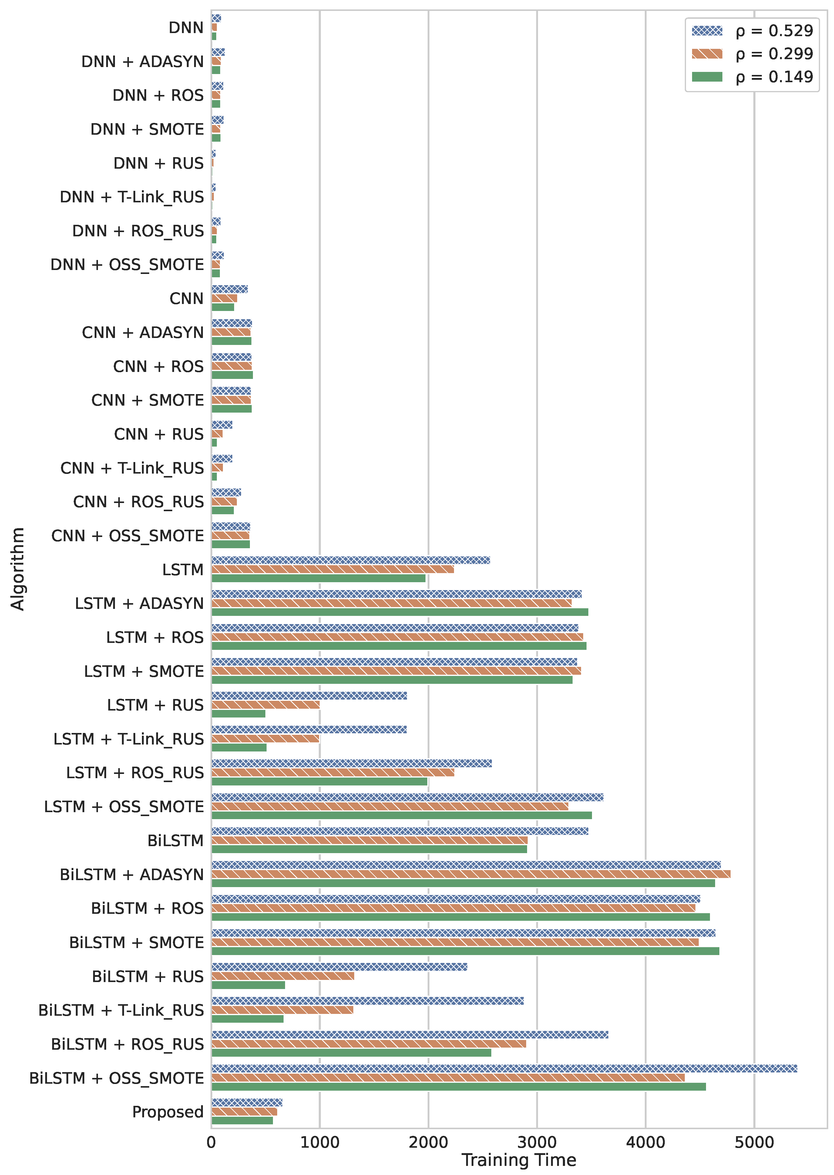
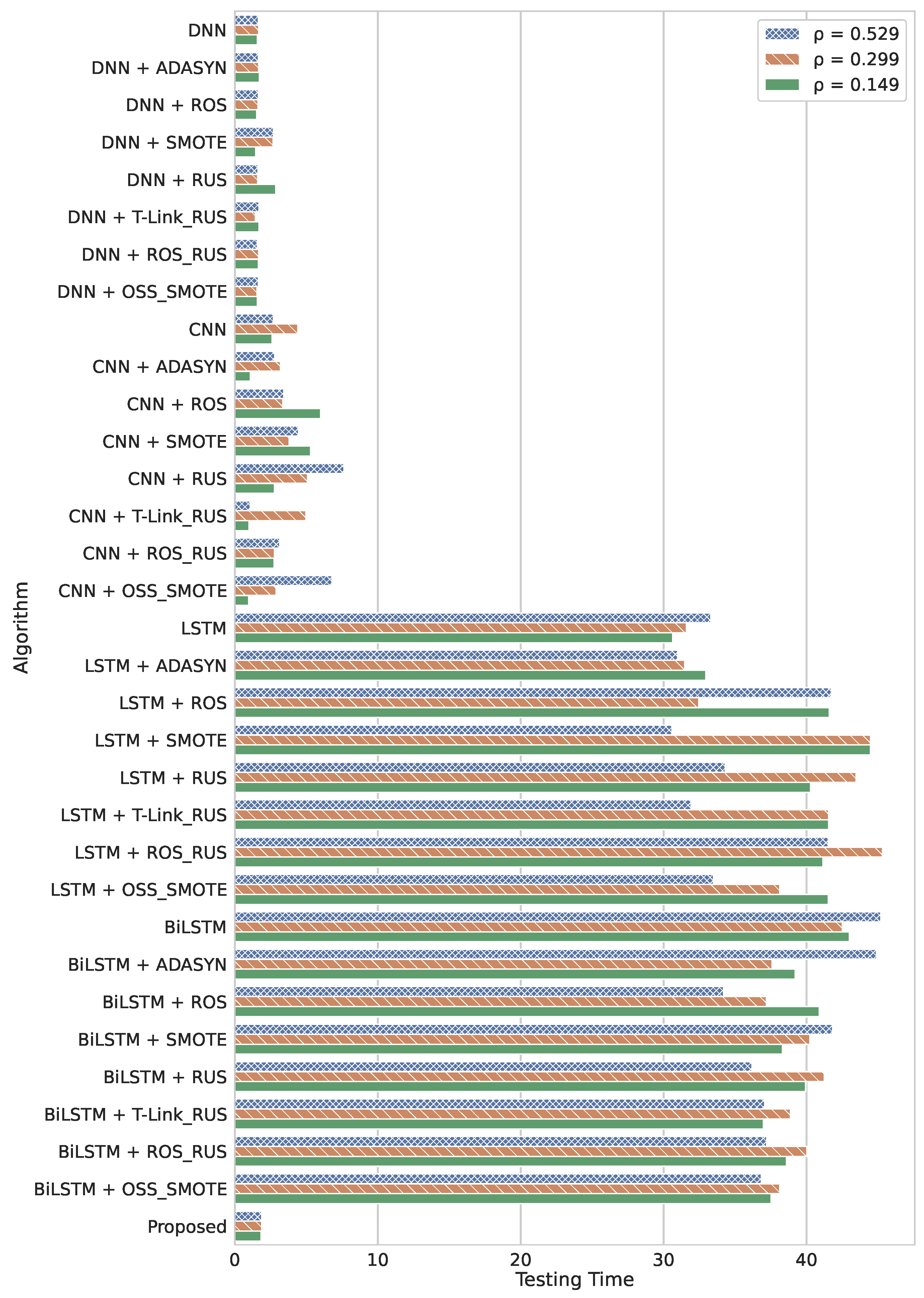
5.1. Timing Performance

5.1.1. Training Time

Since our algorithm represents a state-of-the-art extension in DL solutions for web phishing detection, it is essential to perform a training time analysis according to [12], as this metric represents the bottleneck of several DL classifiers. Figure 2 shows the training time required by each algorithm compared with different $\rho$ values. Furthermore, the influence of the approach used to handle class skew on training time is pointed out, since such a choice affects $\left|S\right|$.

The use of data-level balancing techniques appears to have a significant effect on the required training time. As expected, it increases or decreases by adopting data oversampling or undersampling strategies, respectively. For LSTM and BiLSTM algorithms, the usage of oversampling techniques is very disadvantageous, as a significant increase in training time is found. Furthermore, it is inversely proportional to the actual $\rho$ value. Since training time is very high even in the absence of supporting techniques, oversampling is a very expansive approach. On the other hand, undersampling reduces the required training time proportionally to the actual $\rho$ value. Therefore, the training time of these algorithms is greatly influenced by the amount of data available during the training phase. This trend is expected, since the effective complexity of some DL models also increases with data complexity [18]. This trend is similar for CNN. However, combining CNN with data-balancing techniques is not as disadvantageous as for LSTM and BiLSTM, since the first algorithm requires considerably less training time. The algorithm that takes the shortest training time is DNN. The overall training time required by the combination of DNN with data-level oversampling techniques is the lowest; thus, this approach performs best when considering this aspect.

The training time required by the algorithm proposed in this paper is affected by data availability as it decreases with $\rho$. This trend is expected, as the number of steps in the generic training episode is at most equal to $\left|S\right|$. In general, the DDQN-based classifier training time performances are advantageous compared to those required by LSTM and BiLSTM, but disadvantageous compared to those required by CNN or DNN, even if these were trained on a larger number of samples. In detail, the DDQN-based classifier requires a training time that is about six times higher than DNN combined with oversampling techniques, i.e., despite being trained on a lower number of samples. However, the training time is affected by several factors, such as the choice of hyperparameters, as these affect the effective complexity of a generic DL model [18]. As a consequence, the results obtained in Figure 2 should also refer to the hyperparameter tuning discussed in Section 4.3 and Section 4.4.1.

5.1.2. Testing Time

To complete the timing performance analysis, Figure 3 reports the testing time required by each algorithm compared with different $\rho$ values. Note that the testing time is not affected by the data-level sampling procedure used, as the latter only updates $\left|S\right|$. This figure highlights the following main points: (i) the worst testing time is achieved by LSTM and BiLSTM, which in some cases is greater than 40 s; (ii) the testing time achieved by CNN can reach a maximum of 7.628 s; (iii) the best testing time is achieved by DNN and the proposed algorithm. Therefore, the proposed DDQN-based classifier can provide quicker feedback than widespread DL classifiers, such as CNN, LSTM and BiLSTM.

The overall timing performance analysis includes both training and testing time achieved by the compared algorithms. In this regard, DNN is the most advantageous. The testing time achieved by the proposed DDQN-based classifier makes it the second most advantageous classifier with CNN. Finally, LSTM and BiLSTM do not achieve acceptable results in both cases.

5.2. Classification Performance

The classification performances achieved by each algorithm for different $\rho$ values are reported in Table 5, Table 6 and Table 7. In particular, the best score per evaluated metric is highlighted. According to the problem addressed, it is paramount to focus the analysis on unbalanced classification metric scores, i.e., G-Mean, IBA, F1 score, and AUC, taking into account that each table identifies a different $\rho$ value, i.e., a different problem complexity, in terms of handling class skew. Note that the lower the $\rho$ value, the higher the complexity of the problem.

Table 5 reports the classification metric scores for $\rho =0.529$, identifying the lowest data imbalance. The main findings can be summarized as follows.

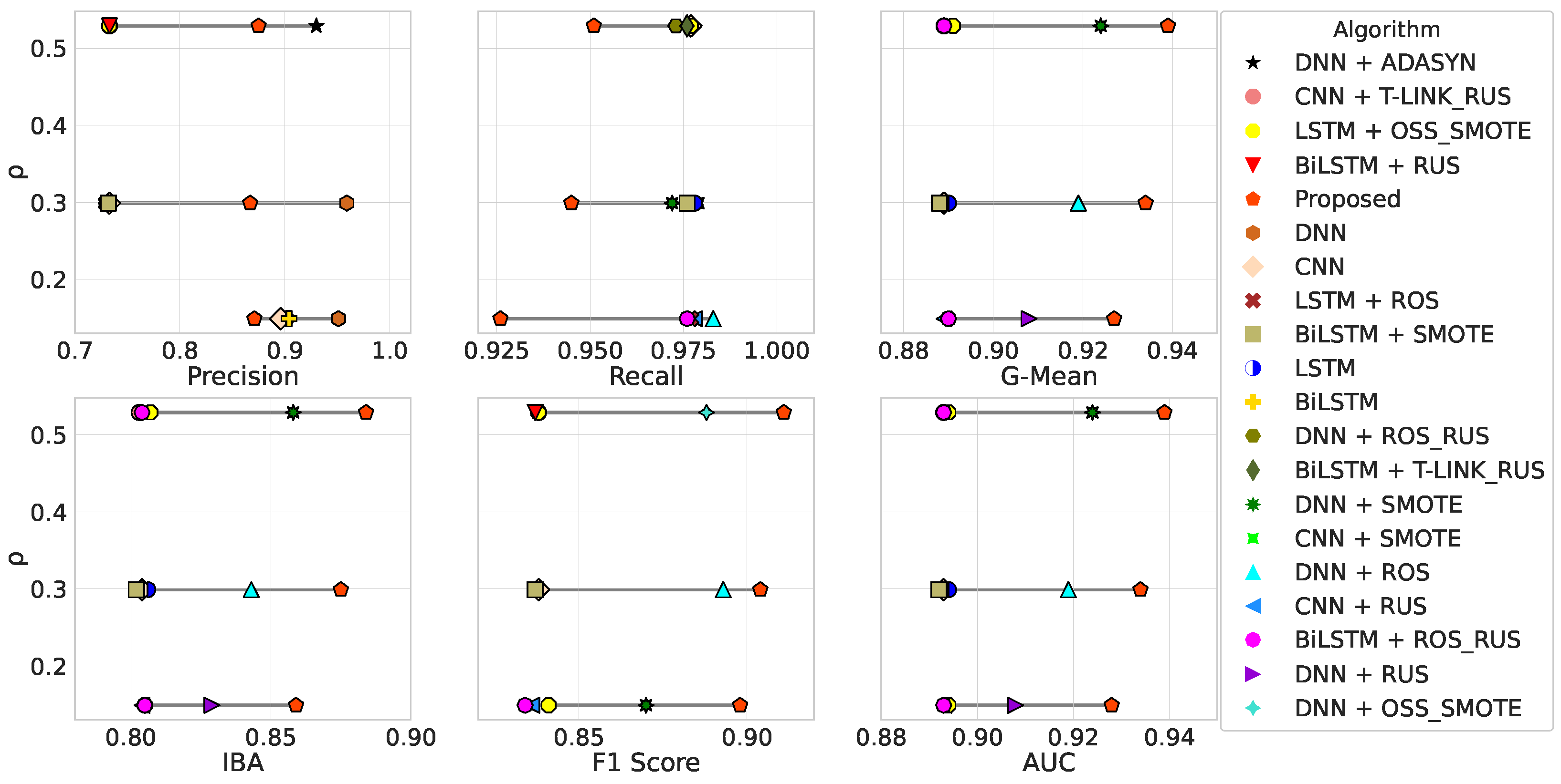
• The CNN, LSTM, and BiLSTM algorithms share the same overall trend in the results obtained. In particular, we can observe that these algorithms are able to minimize the FN (i.e., high recall) score, but they result in many FPs (i.e., low precision) in each case. As a consequence of the low precision value, the maximum F1 score does not reach $84\%$ for any of them. In some cases, CNN and LSTM achieve the best recall score (∼98%) among all algorithms compared. This results in G-Mean and AUC close to $89\%$ and IBA∼0.8. The highest precision score (∼98.5%) is obtained by the LSTM combined with RUS. However, in this case, other metrics show that LSTM becomes a random guessing classifier. Therefore, data imbalance affects the performance achieved by the minority class. Furthermore, the combination with data-level balancing techniques does not improve classification performance. G-Mean and AUC are influenced by a high recall value, while the low IBA reflects that these algorithms are not suitable in any case for dealing with the unbalanced classification problem.
• The DNN algorithm shows good performance, especially when combined with SMOTE or OSS-SMOTE. In these two cases, the high-recall-low-precision trend is less evident since a higher precision value is shown than that achieved by LSTM, BiLSTM and CNN trio. The good trade-off between precision and recall results in an F1 score close to $89\%$. Furthermore, the high recall score results in a high G-Mean (both in the range of $92\%$) and AUC. Finally, an IBA equal to ∼0.86 and ∼0.845 is reached, respectively. Moreover, DNN achieves the best recall score when combined with ROS. However, in this case, the precision score obtained (high value of FP) penalizes the overall unbalanced classification performances. DNN combined with ADASYN works similarly to DNN without prior data-level sampling techniques. Finally, RUS usage leads to worse overall performance unless used in hybrid approaches. For example, T-Link with RUS results in classification metrics very close to those achieved by OSS with SMOTE.
• The proposed DDQN-based classifier outperforms the compared algorithms in terms of G-Mean, IBA, F1 score, and AUC. The highest value of F1 score ($91.1\%$) denotes the best trade-off between precision and recall, equal to $87.5\%$ and $95.1\%$, respectively. The TNR equal to $92.7\%$ results in a very high G-Mean value (∼94%) due to the TPR-TNR balance and the dominance ${\rm Y}$ very close to 0. As a consequence of high ${\rm Y}$, a very high IBA value (∼0.885) is obtained. Finally, the AUC is very close to $0.94$.

For all test cases, Table 6 shows the classification metric scores for the mean unbalanced scenario ($\rho =0.299$). A summary of the main findings is given below.

• The results obtained using CNN, LSTM and BiLSTM show the same low-precision-high-recall of Table 5. In this case, LSTM achieves the best precision score ($99\%$) when combined with ROS-RUS hybrid technique, while the highest recall value ($99\%$) is obtained by LSTM and BiLSTM combined with T-Link-RUS. However, these results are misleading, since other classification metric scores are very poor and denote random guessing classifications performed by all three algorithms. In this case, an F1 score that does not reach $84.5\%$ is obtained, and again G-Mean and AUC are positively influenced by the high recall. Finally, IBA the trend is worse than those achieved by the same algorithms as evaluated in the previous test ($\rho =0.529$).
• DNN does not result in acceptable scores if not combined with data-level sampling techniques. Despite achieving a high precision, the recall score is very low, denoting several FNs. Therefore, in such an experiment, DNN requires using data-level sampling techniques. Performances improve significantly when DNN is combined with ROS, resulting in an F1 score close to $90\%$, a G-Mean∼92%, and an AUC∼0.92. The IBA score is in the range of $0.845$, which is similar to the one achieved by combining DNN with ADASYN. However, the latter is disadvantageous due to a high FP (i.e., low precision score). On the other hand, the usage of ROS and RUS techniques increased FN, while SMOTE and RUS led DNN to results comparable to the low-precision-high-recall trend of CNN, LSTM and BiLSTM. Finally, combining OSS-SMOTE with DNN does not improve performances better than the case in which no data-level balancing technique is adopted.
• In this case, the proposed DDQN-based classifier achieves better G-Mean, IBA, F1 score, and AUC scores than other benchmark algorithms. The F1 score is ∼90.5% due to the trade-off between precision ($86.7\%$) and recall ($94.5\%$). Both TPR and TNR achieved high results ($92.3\%$). Therefore, the high G-Mean score ($93.4\%$) denotes the balance between TPR and TNR. Furthermore, IBA is equal to $0.875$ due to superb dominance ${\rm Y}$, which is equal to $0.022$. Finally, the achieved AUC is $0.934$. The overall performances are very similar to those obtained for the experiment reported in Table 5 i.e., $\rho =0.529$.

Table 7 shows the classification metric test scores obtained using each algorithm for the highest unbalanced scenario (i.e., $\rho =0.149$).

• CNN, LSTM, and BiLSTM confirm the low-precision-high-recall trend already observed in both the above-discussed tests. In this case, BiLSTM achieves the best precision ($98.3\%$) when combined with RUS. However, other classification metric scores reveal that it is a random guess classifier. None of these algorithms achieve a G-Mean equal to $90\%$ and an IBA greater than $0.8$. The maximum F1 score ($83.6\%$) is achieved by combining CNN with RUS and LSTM with ROS, respectively.
• DNN shows good performance in handling class imbalances when combined with SMOTE or RUS. In the first case, a low number of FPs is highlighted by a high precision score ($92.3\%$), which combined with a recall equal to $82.2\%$ results in an F1 score equal to $87\%$. DNN with RUS outperforms DNN with SMOTE in terms of G-Mean, IBA, and AUC due to a high recall (∼93%). Combining DNN with ROS results in the best recall score ($98.3\%$) achieved by all algorithms for this experiment. However, many FPs (precision ∼67%) affect the overall classifier performances. This trend is very similar to the one observed by using ADASYN instead of ROS as an oversampling technique. DNN combined with ROS-RUS or T-Link-RUS results in high FN. Finally, using OSS-SMOTE as a data-level sampling strategy achieves good performances, but a very low IBA value (∼0.7) is obtained.
• The proposed algorithm achieved better results in terms of G-Mean, IBA, F1 score, and AUC compared with other DL algorithms. Despite the limited availability of minority class samples, the proposed DDQN-based classifier is capable of balancing performance in both classes. It achieves ${\rm Y}=-0.002$ since recall = 92.6% and TNR = 92.8%. As a consequence, G-Mean is the average mean between these two values, i.e., $92.7\%$. The IBA of ∼0.86 follows. A very good precision value ($87\%$) positively influences the F1 score, which is close to $90\%$. Finally, AUC denotes good performance thanks to an overall score of $0.928$.

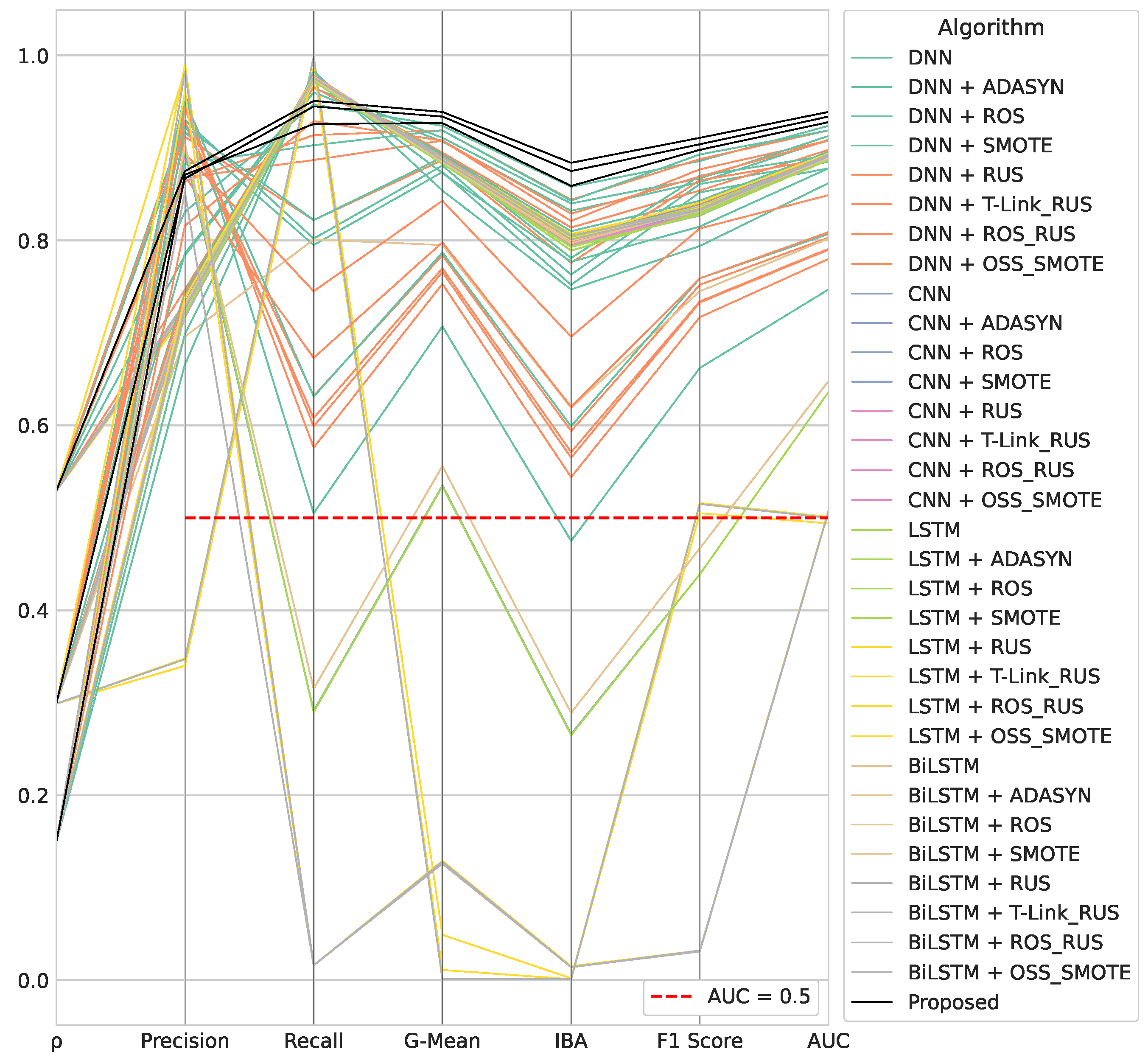
Effectiveness of the Proposed Unbalanced Classifier

The classification performances discussed thus far are summarized using the parallel coordinate plot shown in Figure 4.

Such a graph consists of seven lines. The first line defines the experiment, identified by the $\rho$ value. The remaining six lines represent the classification metric scores achieved by the algorithms tested. As can be seen, the proposed algorithm reached the highest scores for G-Mean, IBA, F1 score, and AUC lines. Furthermore, Figure 4 highlights that although the problem becomes more difficult, i.e., with a lower $\rho$ value, the proposed DDQN-based classifier achieves better problem-specific metric scores than those achieved by the other algorithms when tackling a simpler problem, i.e., with a higher $\rho$ value. This trend is recorded for none of the 32 algorithms compared, denoting the robustness of our algorithm, i.e., its ability to continue operating despite $|S_P|$ decreasing. In this regard, the original dataset is not manipulated by the proposed algorithm, i.e., no synthetic or duplicated data are added to $S_P$, and no data are removed from $S_N$. This is a relevant result that can be achieved using the proposed DDQN-based classifier, since each data manipulation is in contrast with the goal of accurately modeling real-life scenarios.

To better outline the effectiveness of the proposed classifier, we perform two analyses with the aim of pointing out:

• The algorithmic robustness of the best performers for each algorithmic framework, i.e., for each different DL classifier involved (Figure 5). In such an analysis, in the cases where two classifiers belonging to the same framework (same classifier and a different data-level sampling strategy) achieve the same metric score, and the algorithm that appears most frequently in the top performers is selected.
• The comparison between algorithms that outperform the proposed one in precision (Figure 6) and recall (Figure 7) scores, respectively.

Moreover, Figure 4 identifies all classifiers achieving an AUC value close to 0.5 so that the classifier cannot distinguish between malicious and legitimate URLs. Therefore, these are discarded since these cases represent random or constant class predictors. This filtering method helps to reduce the total number of algorithms compared to 24, since this condition is verified for: (i) LSTM combined with RUS for $\rho =0.529$; (ii) LSTM combined with RUS (T-Link-RUS, and ROS-RUS) and BiLSTM combined with T-Link-RUS for $\rho =0.299$; (iii) LSTM combined with RUS and BiLSTM combined with RUS (T-Link-RUS) for $\rho =0.149$.

Figure 5 shows the robustness analysis of the five top performers in each metric evaluated per different DL framework.

This figure highlights that the proposed algorithm is robust to variations in the number of samples within the minority class, i.e., $|S_P|$. This can be appreciated in the constant presence of the proposed DDQN-based classifier in the different metric rankings shown. This is not valid for other top performers that result in performance degradation as $\rho$ varies. Such an analysis can be summarized as follows:

• The DNN combined with ROS is the second-best performer in terms of problem-specific metrics achieved for $\rho =0.299$. However, in the other experiments, it achieves only the best recall score for $\rho =0.149$. DNN combined with RUS is the second-best performer in terms of G-Mean, IBA, and AUC only for $\rho =0.149$. In the same experiment, the same DL classifier achieves the second-best F1 score when combined with SMOTE. However, DNN combined with SMOTE shows an irregular trend, as it alternates good results for different experiments in different metrics. In particular, it achieves the second-best G-Mean, IBA, and AUC for $\rho =0.529$ and the fourth-best recall value for $\rho =0.299$. DNN combined with OSS-SMOTE achieves only the best F1 score score for $\rho =0.529$. DNN without data-level sampling techniques only obtains the best precision scores for $\rho =0.299$ and $\rho =0.149$, respectively. Similarly, DNN combined with ADASYN achieves only the best precision for $\rho =0.529$. Finally, DNN combined with ROS-RUS is the fourth-best performer in the recall ranking for $\rho =0.529$.
• The CNN without data-level sampling strategies is the fourth-best performer in terms of problem-specific metrics achieved for $\rho =0.299$. Furthermore, in the same experiment, it appears in the precision top performers, as well as for $\rho =0.149$. In the case of $\rho =0.529$, it achieves the best recall score. For the latter experiment, CNN combined with T-Link-RUS is ranked as the fourth-best performer in terms of G-Mean, IBA, F1 score, and AUC. The CNN combined with RUS performs similarly for $\rho =0.149$. Moreover, such an algorithm achieves the best recall for $\rho =0.149$. CNN combined with SMOTE achieves only the second-best recall score for $\rho =0.299$.
• The LSTM combined with OSS-SMOTE represents the top performer in each metric evaluated for the DL framework considered in the case of $\rho =0.529$. Furthermore, it achieves the best problem-specific metric scores (again according to the DL framework) for $\rho =0.149$. In the case of $\rho =0.299$, LSTM achieves the second-best recall score without using data-level sampling techniques. The same algorithm results in the best unbalanced classification metrics for its category in such an experiment.
• The BiLSTM achieves the third-best recall score when combined with T-Link-RUS for $\rho =0.529$. In the same experiment, the fourth-best precision and the fifth-best F1 score metrics are obtained by BiLSTM combined with RUS. A similar ranking level is recorded for BiLSTM combined with ROS-RUS for G-Mean, IBA, and AUC metrics. The latter algorithm appears in the same position also in the evaluation of problem-specific metrics for $\rho =0.149$. In the same experiment, it reaches the fourth-best recall score, while the second-best precision is obtained for the BiLSTM without the support of data-level sampling techniques. For $\rho =0.249$, BiLSTM combined with SMOTE is the best performer per category in all metrics evaluated.

Among all the algorithms selected for the benchmark, 20 out of 24 alternate as top performers in all experiments, hence the absence of an alternative robust algorithm to the proposed one is found. In this regard, the results obtained show that the only viable alternative, although with worse performance, is the LSTM combined with OSS-SMOTE. However, it does not appear among the top performers in the second experiment. On the other hand, the algorithm proposed in this paper fulfills the robustness property, resulting in the best problem-specific metrics regardless of $\rho$ value. Therefore, the proposed DDQN-based classifier can effectively continue to operate despite $|S_P|<<|S_N|$. This makes it an ideal algorithm to address the unbalanced web phishing classification problem. However, as shown in Figure 5, the proposed algorithm is clearly not the best performing in terms of precision and recall. Regarding the precision score, it is the second-best performer for $\rho =0.529$ and $\rho =0.299$, respectively. In the case of $\rho =0.149$, it performs worse than the four compared algorithms. On the other hand, it is placed at the fifth position of the recall ranking. To extend such an evaluation, the following analysis focuses on these two metrics, taking into account all the algorithms that outperform the proposed one in precision and recall, respectively. By means of Figure 6 and Figure 7, we want to highlight two main aspects:

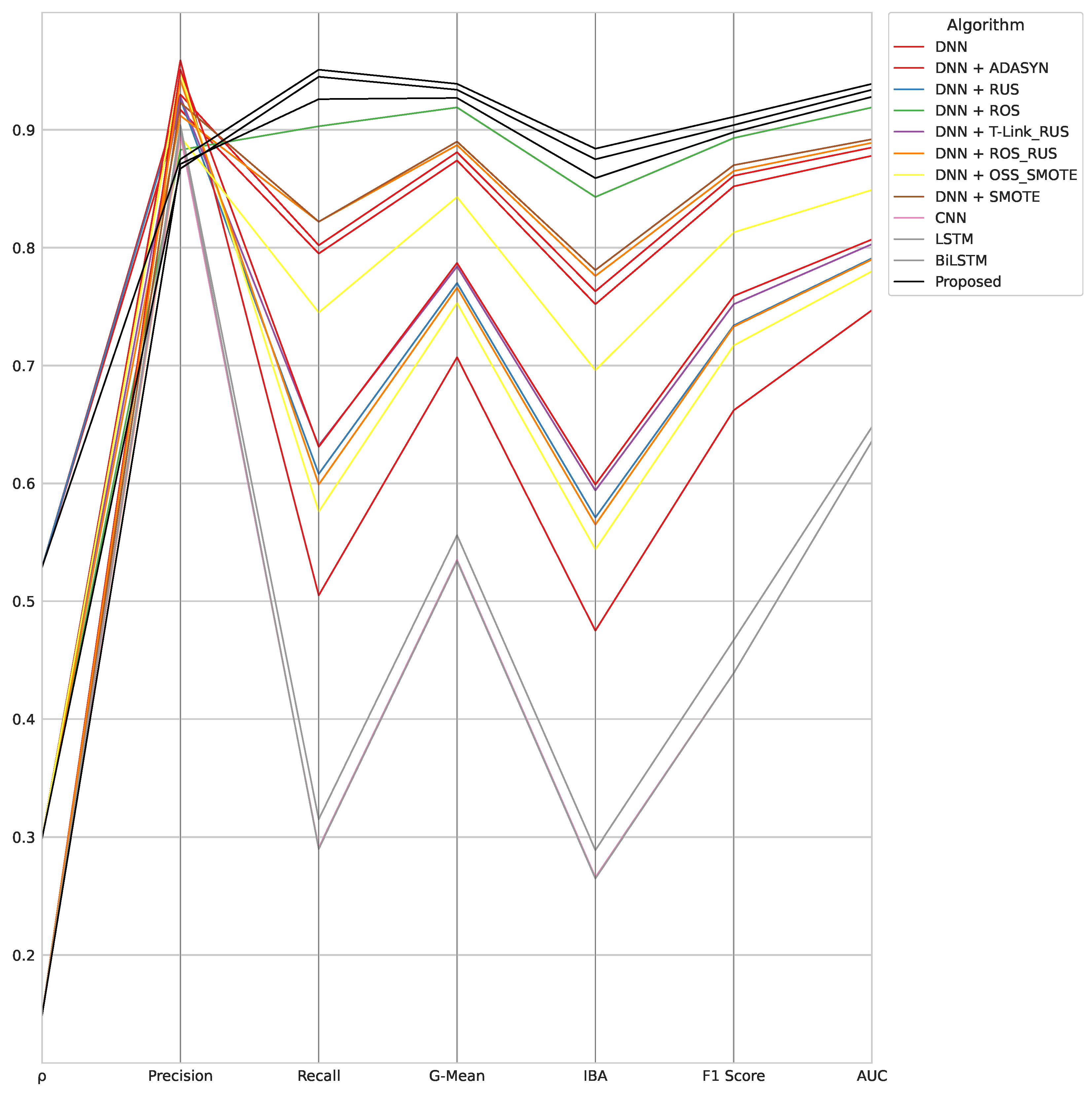
• A compared classifier may be better than the proposed DDQN-based in either precision or recall, but not in both.
• A classifier that identifies a large portion of malicious samples, avoiding FP (FN), i.e., achieving a high precision (recall), is not necessarily satisfactory for addressing the present research problem, which requires a balanced precision-recall trend.

Both Figure 6 and Figure 7 share the same structure as Figure 4, that is, a seven-line parallel coordinate plot, where the first line identifies the experiment, while the remaining lines define the score achieved by a single algorithm in each evaluated metric.

The following main findings can be derived by examining Figure 6:

• The algorithms that outperform the proposed one in precision are divided per experiment as follows:

  –

  DNN, DNN with ADASYN, and DNN with RUS for $\rho =0.529$;

  –

  DNN, DNN with ROS, DNN with T-Link-RUS, DNN with ROS-RUS, and DNN with SMOTE for $\rho =0.299$;

  –

  DNN, DNN with SMOTE, DNN with ROS-RUS, DNN with OSS-SMOTE, CNN, LSTM, BiLSTM for $\rho =0.149$.

  On the other hand, our algorithm scores better on the remaining metrics, including recall, regardless of $\rho$.
• Focusing on classifiers that achieve a higher precision score than the proposed one, a common triangular pattern can be observed in the middle part of the parallel coordinate plot, due to similar recall and IBA scores, and a higher G-Mean value. Therefore, given the triangle built by the trio of points <Recall, G-Mean, IBA>, the higher its height, the greater the influence of precision on the G-Mean, i.e., low FP (high precision, high TNR) and high FN (low recall). As a consequence, the classifier correctly predicts positive samples but is not able to distinguish them from negative ones in more cases. This is a serious issue in real-life applications because legitimate URLs outnumber malicious ones.

Similarly, the main findings derived from Figure 7 can be summarized as follows:

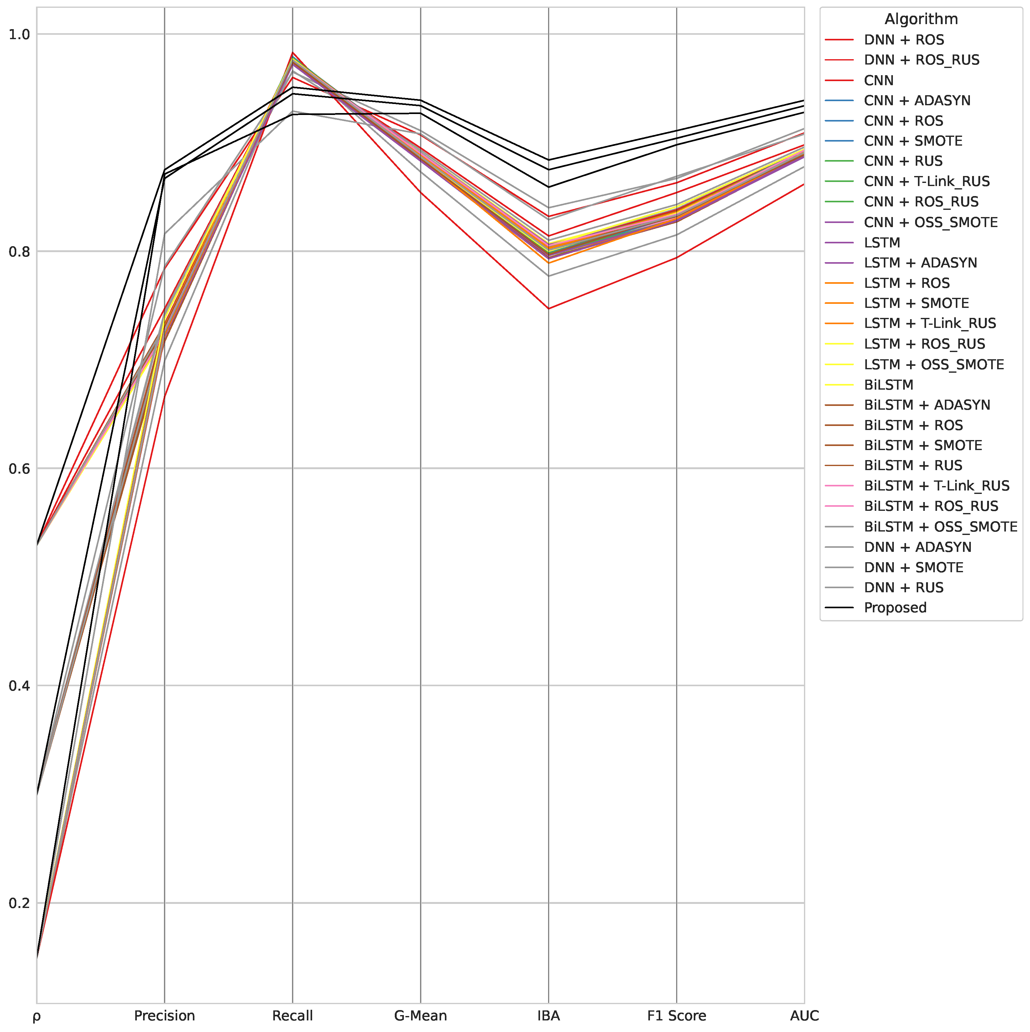
• The algorithms that outperform the proposed one in recall are divided per experiment as follows:

  –

  CNN combined with one of the selected data-level sampling techniques, LSTM with ADASYN, LSTM with ROS, LSTM with SMOTE, LSTM with OSS-SMOTE, and BiLSTM with ADASYN, BiLSTM with ROS, BiLSTM with SMOTE, BiLSTM with ROS-RUS and BiLSTM with OSS-SMOTE in all the experiments;

  –

  CNN, LSTM, and BiLSTM with RUS for $\rho =0.529$ and $\rho =0.299$;

  –

  DNN with ROS, LSTM with ROS-RUS, and LSTM with T-Link-RUS for $\rho =0.529$ and $\rho =0.149$;

  –

  DNN with ADASYN and DNN with RUS for $\rho =0.299$ and $\rho =0.149$;

  –

  DNN with ROS-RUS, BiLSTM, BiLSTM with T-Link-RUS for $\rho =0.529$;

  –

  DNN with SMOTE for $\rho =0.299$.

  On the other hand, our algorithm scores better on the remaining metrics, including precision, regardless of $\rho$.
• Focusing on classifiers that achieve a higher precision score than the proposed one, a triangle formed by the trio of points <Precision, Recall, IBA> having a high height (recall spike very far from precision and IBA) denotes the high influence of the recall on the G-Mean, i.e., low FN (high recall) and high FP (low precision). In these cases, the classifier correctly predicts positive samples but classifies the negative samples as positive in more cases. Such a result is undesired, as in real-life scenarios, navigating to legitimate URLs must be guaranteed.

As a final remark, the proposed algorithm is an effective web phishing unbalanced classifier that performs better than the compared best-precision and best-recall performers in five out of six metrics. Furthermore, the proposed DDQN-based classifier does not result in unbalanced precision–recall trends in the experiments performed; hence, it can classify samples of both despite the class skew, resulting in very promising problem-specific metric scores.

6. Conclusions

Web phishing detection is a critical cybersecurity problem targeting many users. In particular, it can be easily employed as a delivery and weaponization method to exploit human vulnerability, that is, the lack of adequate web phishing awareness training.

This paper extended the state-of-the-art in DL algorithms to address such a problem, taking advantage of the not yet explored DRL framework. In particular, it combined ICMDP to model an unbalanced classification problem, mirroring real-life cases, with a DDQN agent. The proposed DDQN-based classifier has been evaluated by considering three different values of the balancing ratio. The results obtained show its effectiveness in addressing the unbalanced web phishing classification. Despite a significant training time, the classification metrics obtained are very promising without employing prior data sampling techniques, which are not always able to support a classifier in dealing with class skew, as shown by the test results. In addition, the performances obtained are not significantly affected by the variation in the number of samples within the minority class. Therefore, the proposed algorithm represents a robust solution to tackle the unbalanced web phishing classification. Furthermore, a proper hyperparameter optimization procedure can lead to better timing performance. Although the DRL framework has not yet been investigated to address the web phishing detection problem, these results indicate that this field needs to be explored in depth by the scientific community. Among possible future works, the proposed DDQN-based classifier will be used to address other unbalanced classification problems in the cybersecurity domain and will be compared to state-of-the-art shallow learning classifiers combined with data-level sampling techniques.

References

1. Lu, J.; Liu, A.; Dong, F.; Gu, F.; Gama, J.; Zhang, G. Learning under Concept Drift: A Review. IEEE Trans. Knowl. Data Eng. 2019, 31, 2346–2363. [Google Scholar] [CrossRef] [Green Version]
2. Menon, A.G.; Gressel, G. Concept Drift Detection in Phishing Using Autoencoders. In Proceedings of the Machine Learning and Metaheuristics Algorithms, and Applications (SoMMA), Chennai, India, 14–17 October 2020; Thampi, S.M., Piramuthu, S., Li, K.C., Berretti, S., Wozniak, M., Singh, D., Eds.; Springer: Singapore, 2021; pp. 208–220. [Google Scholar] [CrossRef]
3. Raza, M.; Jayasinghe, N.D.; Muslam, M.M.A. A Comprehensive Review on Email Spam Classification using Machine Learning Algorithms. In Proceedings of the 2021 International Conference on Information Networking (ICOIN), Jeju, Republic of Korea, 13–16 January 2021; pp. 327–332. [Google Scholar] [CrossRef]
4. Arulkumaran, K.; Deisenroth, M.P.; Brundage, M.; Bharath, A.A. Deep Reinforcement Learning: A Brief Survey. IEEE Signal Process. Mag. 2017, 34, 26–38. [Google Scholar] [CrossRef] [Green Version]
5. Wang, X.; Wang, S.; Liang, X.; Zhao, D.; Huang, J.; Xu, X.; Dai, B.; Miao, Q. Deep Reinforcement Learning: A Survey. IEEE Trans. Neural Netw. Learn. Syst. 2022, in press. [Google Scholar] [CrossRef] [PubMed]
6. Mnih, V.; Kavukcuoglu, K.; Silver, D.; Graves, A.; Antonoglou, I.; Wierstra, D.; Riedmiller, M. Playing Atari with Deep Reinforcement Learning. arXiv 2013, arXiv:1312.5602. [Google Scholar] [CrossRef]
7. Stekolshchik, R. Some approaches used to overcome overestimation in Deep Reinforcement Learning algorithms. arXiv 2022, arXiv:2006.14167. [Google Scholar] [CrossRef]
8. van Hasselt, H.; Guez, A.; Silver, D. Deep Reinforcement Learning with Double Q-learning. arXiv 2015, arXiv:1509.06461. [Google Scholar] [CrossRef]
9. Lopez-Martin, M.; Carro, B.; Sanchez-Esguevillas, A. Application of deep reinforcement learning to intrusion detection for supervised problems. Expert Syst. Appl. 2020, 141, 112963. [Google Scholar] [CrossRef]
10. Nguyen, T.T.; Reddi, V.J. Deep Reinforcement Learning for Cyber Security. IEEE Trans. Neural Netw. Learn. Syst. 2021, in press. [Google Scholar] [CrossRef]
11. Sarker, I.H. Deep Cybersecurity: A Comprehensive Overview from Neural Network and Deep Learning Perspective. SN Comput. Sci. 2021, 2, 154. [Google Scholar] [CrossRef]
12. Do, N.Q.; Selamat, A.; Krejcar, O.; Herrera-Viedma, E.; Fujita, H. Deep Learning for Phishing Detection: Taxonomy, Current Challenges and Future Directions. IEEE Access 2022, 10, 36429–36463. [Google Scholar] [CrossRef]
13. Chatterjee, M.; Namin, A.S. Detecting Phishing Websites through Deep Reinforcement Learning. In Proceedings of the 2019 IEEE 43rd Annual Computer Software and Applications Conference (COMPSAC), Milwaukee, WI, USA, 15–19 July 2019; Volume 2, pp. 227–232. [Google Scholar] [CrossRef]
14. Do, N.Q.; Selamat, A.; Krejcar, O.; Yokoi, T.; Fujita, H. Phishing Webpage Classification via Deep Learning-Based Algorithms: An Empirical Study. Appl. Sci. 2021, 11, 9210. [Google Scholar] [CrossRef]
15. Thabtah, F.; Hammoud, S.; Kamalov, F.; Gonsalves, A. Data imbalance in classification: Experimental evaluation. Inf. Sci. 2020, 513, 429–441. [Google Scholar] [CrossRef]
16. Dablain, D.; Krawczyk, B.; Chawla, N.V. DeepSMOTE: Fusing Deep Learning and SMOTE for Imbalanced Data. IEEE Trans. Neural Netw. Learn. Syst. 2022, in press. [Google Scholar] [CrossRef] [PubMed]
17. Johnson, J.; Khoshgoftaar, T. Survey on deep learning with class imbalance. J. Big Data 2019, 6, 27. [Google Scholar] [CrossRef] [Green Version]
18. Hu, X.; Chu, L.; Pei, J.; Liu, W.; Bian, J. Model complexity of deep learning: A survey. Knowl. Inf. Syst. 2021, 63, 2585–2619. [Google Scholar] [CrossRef]
19. Siddhesh Vijay, J.; Kulkarni, K.; Arya, A. Metaheuristic Optimization of Neural Networks for Phishing Detection. In Proceedings of the 2022 3rd International Conference for Emerging Technology (INCET), Belgaum, India, 27–29 May 2022; pp. 1–5. [Google Scholar] [CrossRef]
20. Ul Hassan, I.; Ali, R.H.; Ul Abideen, Z.; Khan, T.A.; Kouatly, R. Significance of machine learning for detection of malicious websites on an unbalanced dataset. Digital 2022, 2, 501–519. [Google Scholar] [CrossRef]
21. Pristyanto, Y.; Dahlan, A. Hybrid Resampling for Imbalanced Class Handling on Web Phishing Classification Dataset. In Proceedings of the 2019 4th International Conference on Information Technology, Information Systems and Electrical Engineering (ICITISEE), Yogyakarta, Indonesia, 20–21 November 2019; pp. 401–406. [Google Scholar] [CrossRef]
22. Lin, E.; Chen, Q.; Qi, X. Deep Reinforcement Learning for Imbalanced Classification. Appl. Intell. 2020, 50, 2488–2502. [Google Scholar] [CrossRef] [Green Version]
23. Jang, B.; Kim, M.; Harerimana, G.; Kim, J.W. Q-Learning Algorithms: A Comprehensive Classification and Applications. IEEE Access 2019, 7, 133653–133667. [Google Scholar] [CrossRef]
24. Hasselt, H. Double Q-learning. In Proceedings of the Advances in Neural Information Processing Systems, Vancouver, BC, Canada, 6–11 December 2010; Lafferty, J., Williams, C., Shawe-Taylor, J., Zemel, R., Culotta, A., Eds.; Curran Associates, Inc.: La Jolla, CA, USA; Volume 2, pp. 2613–2621. [Google Scholar]
25. Mishra, P.; Varadharajan, V.; Tupakula, U.; Pilli, E.S. A Detailed Investigation and Analysis of Using Machine Learning Techniques for Intrusion Detection. IEEE Commun. Surv. Tutorials 2019, 21, 686–728. [Google Scholar] [CrossRef]
26. Sewak, M.; Sahay, S.K.; Rathore, H. Deep Reinforcement Learning in the Advanced Cybersecurity Threat Detection and Protection. Inf. Syst. Front. 2022, 25, 589–611. [Google Scholar] [CrossRef]
27. Liu, Y.; Dong, M.; Ota, K.; Li, J.; Wu, J. Deep Reinforcement Learning based Smart Mitigation of DDoS Flooding in Software-Defined Networks. In Proceedings of the 2018 IEEE 23rd International Workshop on Computer Aided Modeling and Design of Communication Links and Networks (CAMAD), Barcelona, Spain, 17–19 September 2018; pp. 1–6. [Google Scholar] [CrossRef]
28. Shi, G.; He, G. Collaborative Multi-agent Reinforcement Learning for Intrusion Detection. In Proceedings of the 2021 7th IEEE International Conference on Network Intelligence and Digital Content (IC-NIDC), Beijing, China, 17–19 November 2021; pp. 245–249. [Google Scholar] [CrossRef]
29. Dong, S.; Xia, Y.; Peng, T. Network Abnormal Traffic Detection Model Based on Semi-Supervised Deep Reinforcement Learning. IEEE Trans. Netw. Serv. Manag. 2021, 18, 4197–4212. [Google Scholar] [CrossRef]
30. Gülmez, H.; Angin, P. A Study on the Efficacy of Deep Reinforcement Learning for Intrusion Detection. Sak. Univ. J. Comput. Inf. Sci. 2020, 4, 834048. [Google Scholar] [CrossRef]
31. Hsu, Y.F.; Matsuoka, M. A Deep Reinforcement Learning Approach for Anomaly Network Intrusion Detection System. In Proceedings of the 2020 IEEE 9th International Conference on Cloud Networking (CloudNet), Virtual, 9–11 November 2020; pp. 1–6. [Google Scholar] [CrossRef]
32. Sujatha, V.; Prasanna, K.L.; Niharika, K.; Charishma, V.; Sai, K.B. Network Intrusion Detection using Deep Reinforcement Learning. In Proceedings of the 2023 7th International Conference on Computing Methodologies and Communication (ICCMC), Erode, India, 23–25 February 2023; pp. 1146–1150. [Google Scholar] [CrossRef]
33. Caminero, G.; Lopez-Martin, M.; Carro, B. Adversarial environment reinforcement learning algorithm for intrusion detection. Comput. Netw. 2019, 159, 96–109. [Google Scholar] [CrossRef]
34. Yang, B.; Arshad, M.H.; Zhao, Q. Packet-Level and Flow-Level Network Intrusion Detection Based on Reinforcement Learning and Adversarial Training. Algorithms 2022, 15, 453. [Google Scholar] [CrossRef]
35. Alavizadeh, H.; Alavizadeh, H.; Jang-Jaccard, J. Deep Q-Learning Based Reinforcement Learning Approach for Network Intrusion Detection. Computers 2022, 11, 41. [Google Scholar] [CrossRef]
36. Wheelus, C.; Bou-Harb, E.; Zhu, X. Tackling Class Imbalance in Cyber Security Datasets. In Proceedings of the 2018 IEEE International Conference on Information Reuse and Integration (IRI), Salt Lake City, UT, USA, 6–9 July 2018; pp. 229–232. [Google Scholar] [CrossRef]
37. Abdelkhalek, A.; Mashaly, M. Addressing the class imbalance problem in network intrusion detection systems using data resampling and deep learning. J. Supercomput. 2023, 79, 10611–10644. [Google Scholar] [CrossRef]
38. Fdez-Glez, J.; Ruano-Ordás, D.; Fdez-Riverola, F.; Méndez, J.R.; Pavón, R.; Laza, R. Analyzing the impact of unbalanced data on web spam classification. In Proceedings of the Distributed Computing and Artificial Intelligence, 12th International Conference, Skövde, Sweden, 21–23 September 2015; Springer: Berlin/Heidelberg, Germany, 2015; Volume 373, pp. 243–250. [Google Scholar] [CrossRef]
39. Livara, A.; Hernandez, R. An Empirical Analysis of Machine Learning Techniques in Phishing E-mail detection. In Proceedings of the 2022 International Conference for Advancement in Technology (ICONAT), Goa, India, 21–22 January 2022; pp. 1–6. [Google Scholar] [CrossRef]
40. Gutierrez, C.N.; Kim, T.; Corte, R.D.; Avery, J.; Goldwasser, D.; Cinque, M.; Bagchi, S. Learning from the Ones that Got Away: Detecting New Forms of Phishing Attacks. IEEE Trans. Dependable Secur. Comput. 2018, 15, 988–1001. [Google Scholar] [CrossRef]
41. Ahsan, M.; Gomes, R.; Denton, A. SMOTE Implementation on Phishing Data to Enhance Cybersecurity. In Proceedings of the 2018 IEEE International Conference on Electro/Information Technology (EIT), Rochester, MI, USA, 3–5 May 2018; pp. 531–536. [Google Scholar] [CrossRef]
42. Priya, S.; Uthra, R.A. Deep learning framework for handling concept drift and class imbalanced complex decision-making on streaming data. Complex Intell. Syst. 2021, in press. [Google Scholar] [CrossRef]
43. Abdul Samad, S.R.; Balasubaramanian, S.; Al-Kaabi, A.S.; Sharma, B.; Chowdhury, S.; Mehbodniya, A.; Webber, J.L.; Bostani, A. Analysis of the Performance Impact of Fine-Tuned Machine Learning Model for Phishing URL Detection. Electronics 2023, 12, 1642. [Google Scholar] [CrossRef]
44. He, S.; Li, B.; Peng, H.; Xin, J.; Zhang, E. An Effective Cost-Sensitive XGBoost Method for Malicious URLs Detection in Imbalanced Dataset. IEEE Access 2021, 9, 93089–93096. [Google Scholar] [CrossRef]
45. Tan, G.; Zhang, P.; Liu, Q.; Liu, X.; Zhu, C.; Dou, F. Adaptive Malicious URL Detection: Learning in the Presence of Concept Drifts. In Proceedings of the 2018 17th IEEE International Conference on Trust, Security and Privacy in Computing and Communications/12th IEEE International Conference on Big Data Science and Engineering (TrustCom/BigDataSE), New York, NY, USA, 1–3 August 2018; pp. 737–743. [Google Scholar] [CrossRef]
46. Zhao, C.; Xin, Y.; Li, X.; Yang, Y.; Chen, Y. A Heterogeneous Ensemble Learning Framework for Spam Detection in Social Networks with Imbalanced Data. Appl. Sci. 2020, 10, 936. [Google Scholar] [CrossRef] [Green Version]
47. Bu, S.J.; Cho, S.B. Deep Character-Level Anomaly Detection Based on a Convolutional Autoencoder for Zero-Day Phishing URL Detection. Electronics 2021, 10, 1492. [Google Scholar] [CrossRef]
48. Xiao, X.; Xiao, W.; Zhang, D.; Zhang, B.; Hu, G.; Li, Q.; Xia, S. Phishing websites detection via CNN and multi-head self-attention on imbalanced datasets. Comput. Secur. 2021, 108, 102372. [Google Scholar] [CrossRef]
49. Anand, A.; Gorde, K.; Antony Moniz, J.R.; Park, N.; Chakraborty, T.; Chu, B.T. Phishing URL Detection with Oversampling based on Text Generative Adversarial Networks. In Proceedings of the 2018 IEEE International Conference on Big Data (Big Data), Seattle, WA, USA, 10–13 December 2018; pp. 1168–1177. [Google Scholar] [CrossRef]
50. Naim, O.; Cohen, D.; Ben-Gal, I. Malicious website identification using design attribute learning. Int. J. Inf. Secur. 2023, in press. [Google Scholar] [CrossRef]
51. Vrbančič, G.; Fister, I., Jr.; Podgorelec, V. Datasets for phishing websites detection. Data Brief 2020, 33, 106438. [Google Scholar] [CrossRef]
52. Vrbančič, G. Phishing Websites Dataset. 2020. Available online: https://data.mendeley.com/datasets/72ptz43s9v/1 (accessed on 30 November 2022).
53. Safi, A.; Singh, S. A systematic literature review on phishing website detection techniques. J. King Saud Univ.-Comput. Inf. Sci. 2023, 35, 590–611. [Google Scholar] [CrossRef]
54. Wang, G.; Wong, K.W.; Lu, J. AUC-Based Extreme Learning Machines for Supervised and Semi-Supervised Imbalanced Classification. IEEE Trans. Syst. Man Cybern. Syst. 2021, 51, 7919–7930. [Google Scholar] [CrossRef]
55. García, V.; Mollineda, R.; Sánchez, J. Index of Balanced Accuracy: A Performance Measure for Skewed Class Distributions. In Proceedings of the Pattern Recognition and Image Analysis: 4th Iberian Conference, Póvoa de Varzim, Portugal, 10–12 June 2009; Springer: Berlin/Heidelberg, Germany, 2009; Volume 5524, pp. 441–448. [Google Scholar] [CrossRef] [Green Version]
56. Lemaître, G.; Nogueira, F.; Aridas, C.K. Imbalanced-learn: A Python Toolbox to Tackle the Curse of Imbalanced Datasets in Machine Learning. J. Mach. Learn. Res. 2017, 18, 1–5. [Google Scholar]
57. van den Berg, T. imbDRL: Imbalanced Classification with Deep Reinforcement Learning. 2021. Available online: https://github.com/Denbergvanthijs/imbDRL (accessed on 16 November 2022).
58. McKinney, W. Data Structures for Statistical Computing in Python. In Proceedings of the 9th Python in Science Conference, Austin, TX, USA, 28 June–3 July 2010; van der Walt, S., Millman, J., Eds.; pp. 56–61. [Google Scholar] [CrossRef] [Green Version]
59. Harris, C.R.; Millman, K.J.; van der Walt, S.J.; Gommers, R.; Virtanen, P.; Cournapeau, D.; Wieser, E.; Taylor, J.; Berg, S.; Smith, N.J.; et al. Array programming with NumPy. Nature 2020, 585, 357–362. [Google Scholar] [CrossRef]
60. Brockman, G.; Cheung, V.; Pettersson, L.; Schneider, J.; Schulman, J.; Tang, J.; Zaremba, W. OpenAI Gym. arXiv 2016, arXiv:1606.01540. [Google Scholar] [CrossRef]
61. Abadi, M.; Agarwal, A.; Barham, P.; Brevdo, E.; Chen, Z.; Citro, C.; Corrado, G.S.; Davis, A.; Dean, J.; Devin, M.; et al. TensorFlow: Large-Scale Machine Learning on Heterogeneous Systems. 2015. Available online: https://www.tensorflow.org/ (accessed on 18 January 2023).
62. Pedregosa, F.; Varoquaux, G.; Gramfort, A.; Michel, V.; Thirion, B.; Grisel, O.; Blondel, M.; Prettenhofer, P.; Weiss, R.; Dubourg, V.; et al. Scikit-learn: Machine Learning in Python. J. Mach. Learn. Res. 2011, 12, 2825–2830. [Google Scholar]
63. Yerima, S.Y.; Alzaylaee, M.K. High Accuracy Phishing Detection Based on Convolutional Neural Networks. In Proceedings of the 2020 3rd International Conference on Computer Applications & Information Security (ICCAIS), Riyadh, Saudi Arabia, 19–21 March 2020; pp. 1–6. [Google Scholar] [CrossRef]
64. Hochreiter, S.; Schmidhuber, J. Long Short-Term Memory. Neural Comput. 1997, 9, 1735–1780. [Google Scholar] [CrossRef]
65. Schuster, M.; Paliwal, K. Bidirectional recurrent neural networks. IEEE Trans. Signal Process. 1997, 45, 2673–2681. [Google Scholar] [CrossRef] [Green Version]
66. Chawla, N.V.; Bowyer, K.W.; Hall, L.O.; Kegelmeyer, W.P. SMOTE: Synthetic Minority Over-sampling Technique. J. Artif. Intell. Res. 2002, 16, 321–357. [Google Scholar] [CrossRef]
67. He, H.; Bai, Y.; Garcia, E.A.; Li, S. ADASYN: Adaptive synthetic sampling approach for imbalanced learning. In Proceedings of the 2008 IEEE International Joint Conference on Neural Networks (IEEE World Congress on Computational Intelligence), Hong Kong, China, 1–8 June 2008; pp. 1322–1328. [Google Scholar] [CrossRef] [Green Version]
68. Elhassan, T.; Aljurf, M. Classification of imbalance data using tomek link (t-link) combined with random under-sampling (rus) as a data reduction method. Glob. J. Technol. Optim. 2016, 1, 111. [Google Scholar] [CrossRef]
69. Kubat, M.; Matwin, S. Addressing the curse of imbalanced training sets: One-sided selection. In Proceedings of the Fourteenth International Conference on Machine Learning (ICML ’97) Citeseer, San Francisco, CA, USA, 8–12 July 1997; Volume 97, pp. 179–186. [Google Scholar]
70. Johnson, J.M.; Khoshgoftaar, T.M. Deep Learning and Data Sampling with Imbalanced Big Data. In Proceedings of the 2019 IEEE 20th International Conference on Information Reuse and Integration for Data Science (IRI), Los Angeles, CA, USA, 30 July–1 August 2019; pp. 175–183. [Google Scholar] [CrossRef]
71. Johnson, J.M.; Khoshgoftaar, T.M. The effects of data sampling with deep learning and highly imbalanced big data. Inf. Syst. Front. 2020, 22, 1113–1131. [Google Scholar] [CrossRef]
Figure 1. Proposed classifier workflow. In this figure, π * represents the optimal classification policy learned by the agent.
Computers 12 00118 g001
Figure 2. Training time (in seconds) required by the algorithms compared for different test cases.
Computers 12 00118 g002
Figure 3. Testing time (in seconds) required by the algorithms compared for different test cases.
Computers 12 00118 g003
Figure 4. Overview of the overall classification performance achieved by each compared algorithm.
Computers 12 00118 g004
Figure 5. Robustness analysis of the five best DL classifiers per different DL framework for each test case.
Computers 12 00118 g005
Figure 6. Comparison between the proposed algorithm and all others achieving a higher precision score.
Computers 12 00118 g006
Figure 7. Comparison between the proposed algorithm and all others achieving a higher recall score.
Computers 12 00118 g007