Author Contributions
Conceptualization, T.B.R. and P.B.; methodology, T.B.R.; software, T.B.R.; validation, T.B.R. and P.B.; formal analysis, T.B.R.; investigation, T.B.R.; writing—original draft preparation, T.B.R. and P.B.; writing—review and editing, T.B.R., P.B., S.W. and F.S.; visualization, T.B.R.; supervision, S.W. and F.S.; project administration, S.W. and F.S. All authors have read and agreed to the published version of the manuscript.
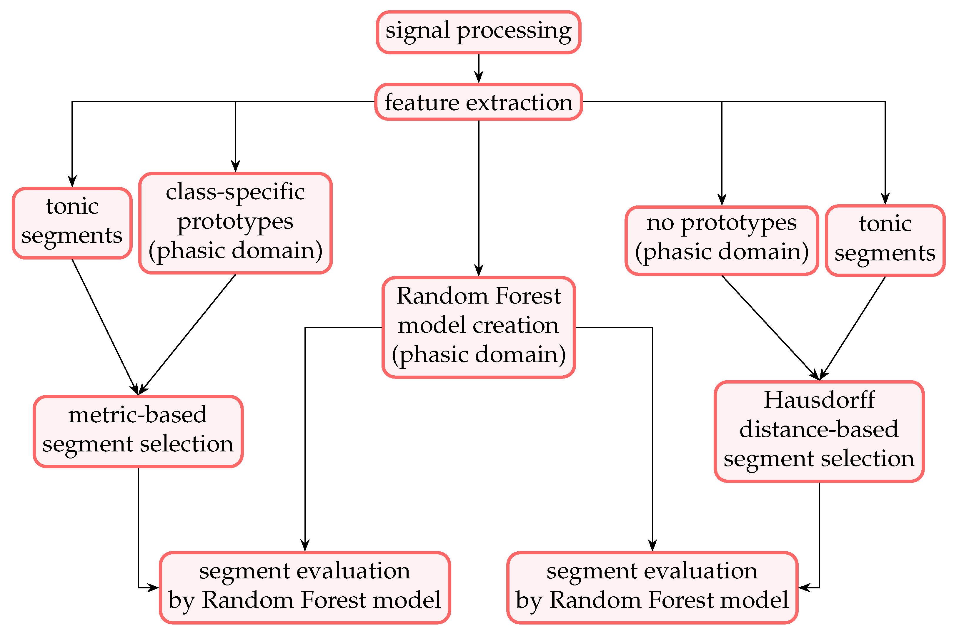
Figure 1.
Complete process of the evaluated experiments. The random forest model is trained solely on the phasic domain samples. The evaluation follows one of the two available branches. The left branch represents the prototype-based evaluation, whereas the right branch represents the Hausdorff distance-based evaluation. Note that the Hausdorff distance is the only evaluated metric in which no prototypes are computed. The knowledge transfer from the phasic domain to the tonic domain is performed by the evaluation of the individual segments.
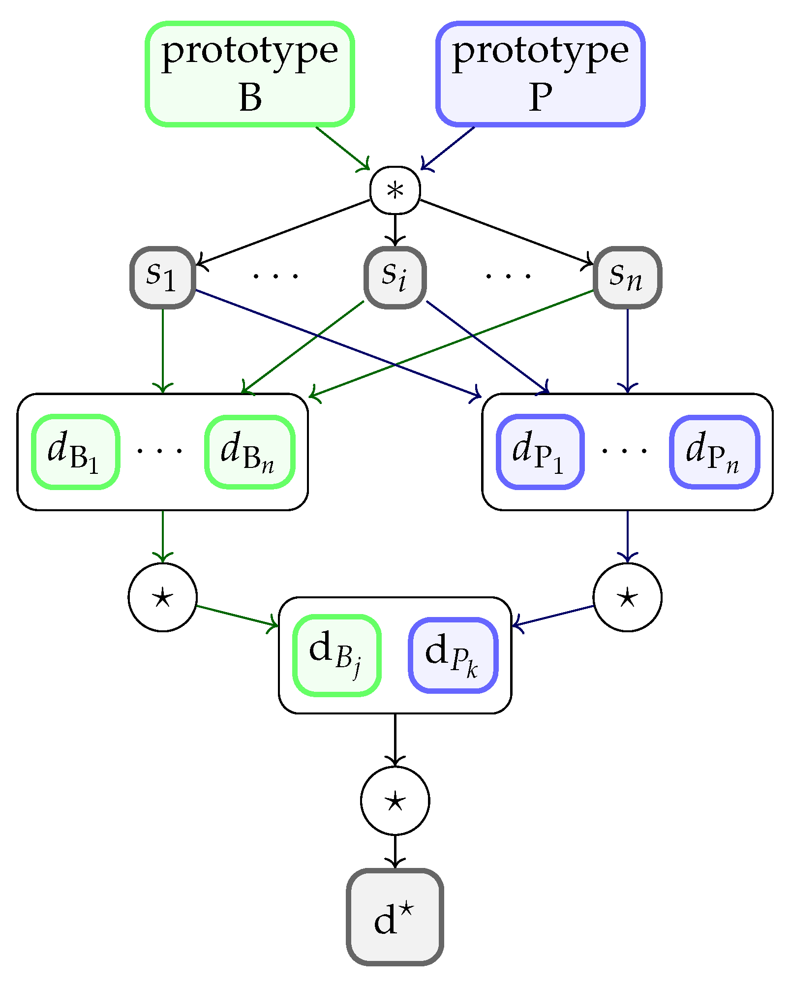
Figure 2.
Segment selection process. The *-operator denotes the metric-based distance computation between the prototypes and each segment . Parameters and denote the resulting distance values for the baseline (B) and pain (P) prototypes, respectively. The ⋆-operator denotes the selection operator (here: minimum) performed on the vectors of the obtained values. and denote the lowest distances to the prototypes. The overall lowest distance is obtained when the ⋆-operator is applied to and . The segment, to which the value belongs to, is selected and evaluated by the model. (Note that this approach is applied in combination with all evaluated metrics defined above, except for the Hausdorff distance).
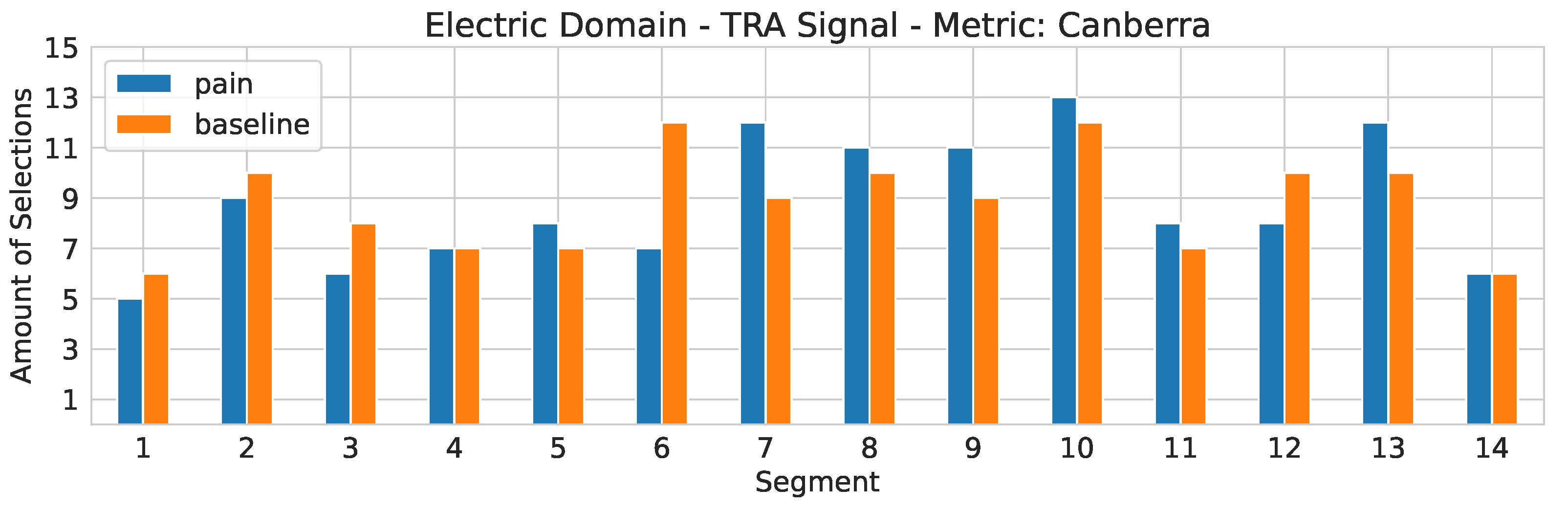
Figure 3.
Electric domain. The segment selection frequency for the TRA signal in combination with the Canberra metric. On the x-axis, the segment number is depicted. The y-axis represents the segment counter.
Figure 3.
Electric domain. The segment selection frequency for the TRA signal in combination with the Canberra metric. On the x-axis, the segment number is depicted. The y-axis represents the segment counter.
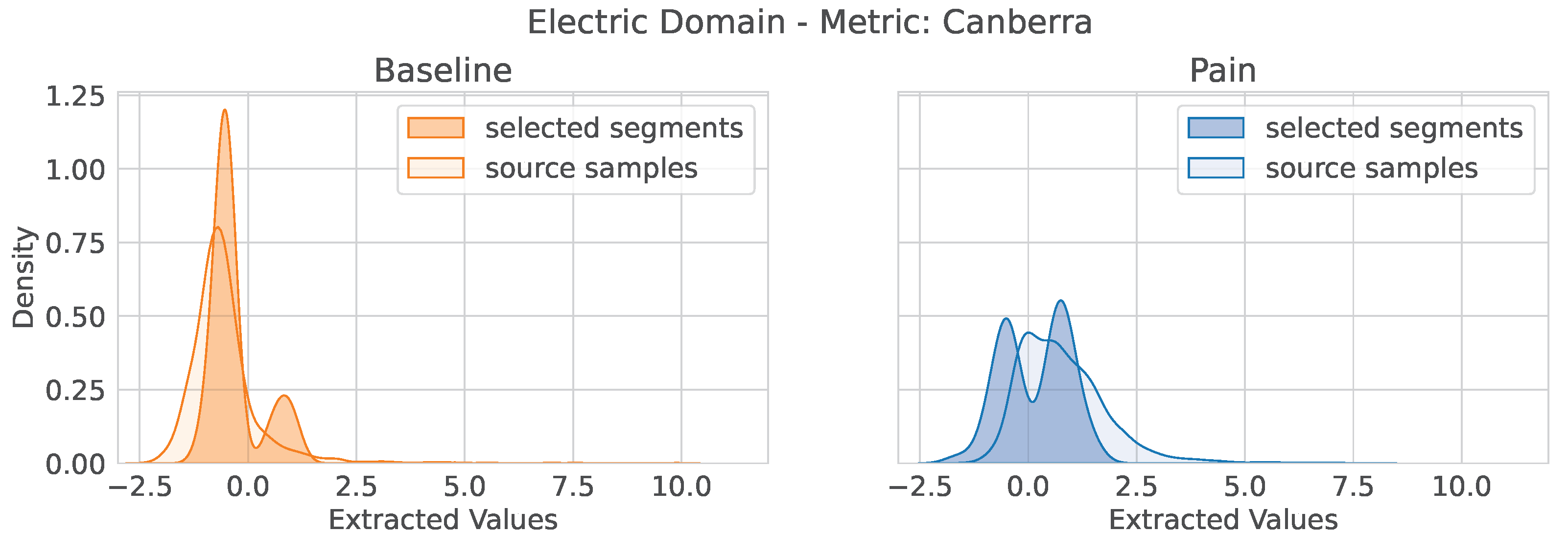
Figure 4.
Electric domain: TRA signal—Canberra metric. Distribution of extracted feature values for the feature trapezius_second_derivative_features_signal_std of the TRA signal in combination with the selected segments with the Canberra metric and the distribution of the source domain samples (phasic domain). (Left) Value distributions for the baseline stimuli. (Right) Value distributions of the pain stimuli.
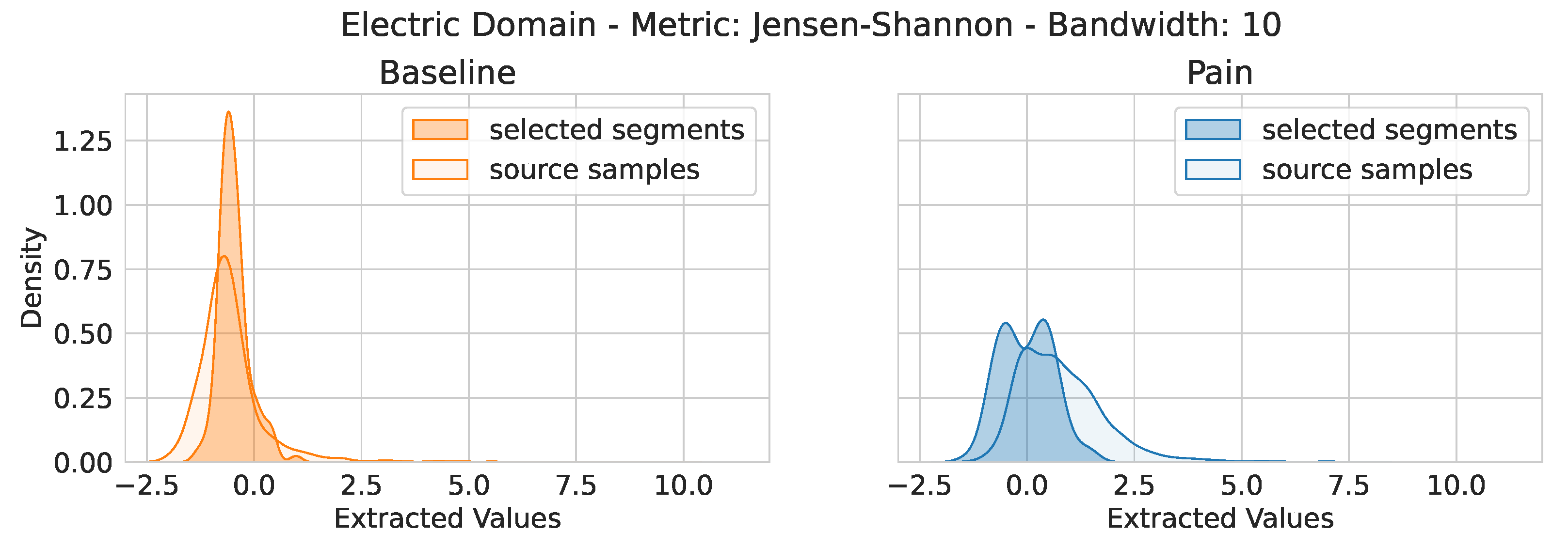
Figure 5.
Electric domain: TRA signal—Jensen–Shannon metric with bandwidth set to ten. Distribution of extracted feature values for the feature trapezius_second_derivative_features_signal_std of the TRA signal in combination with the selected segments with the Canberra metric and the distribution of the source domain samples (phasic domain). (Left) Value distributions for the baseline stimuli. (Right) Value distributions of the pain stimuli.
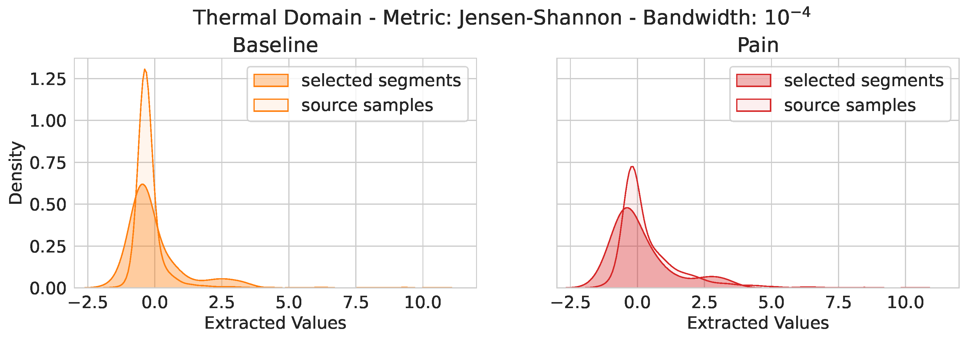
Figure 6.
Thermal Domain: TRA signal—Jensen–Shannon metric with a bandwidth of . Distribution of extracted feature values for the feature trapezius_second_derivative_features_signal_ split_equal_part_std of the TRA signal in combination with the selected segments with the Canberra metric and the distribution of the source domain samples (phasic domain). (Left) Value distributions for the baseline stimuli. (Right) Value distributions of the pain stimuli.
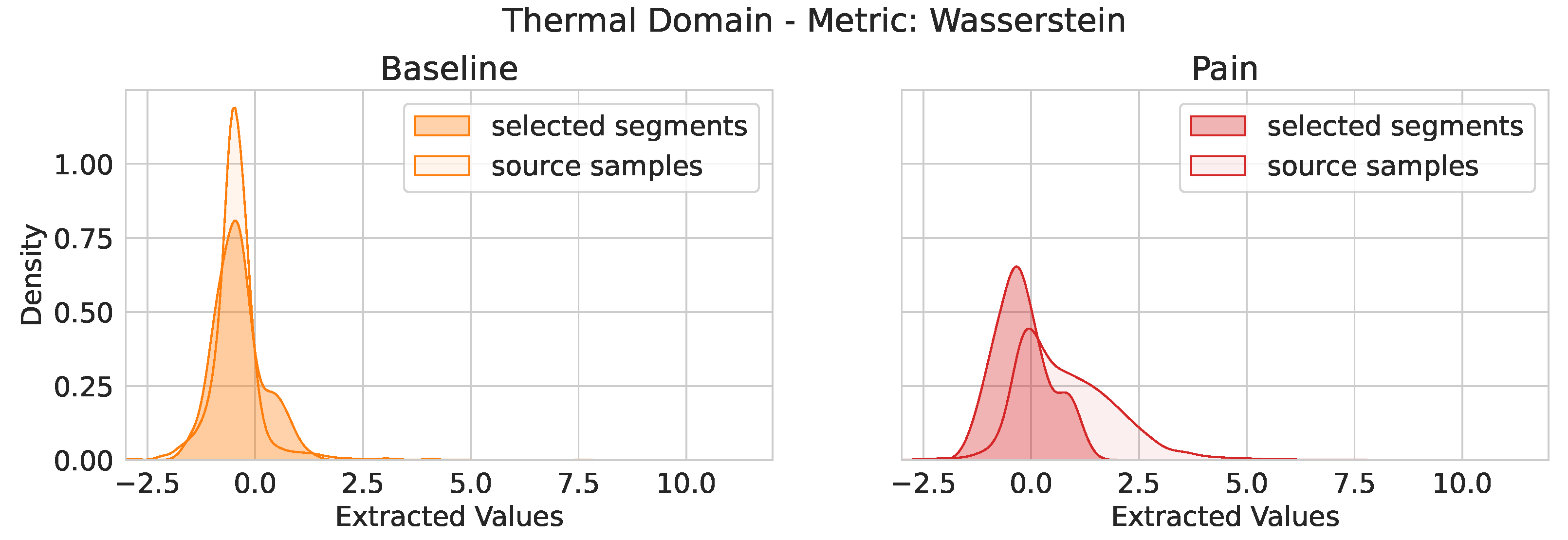
Figure 7.
Thermal Domain: EDA signal—Wasserstein metric. Distribution of extracted feature values for the feature trapezius_mean_value_first_diff of the EDA signal in combination with the selected segments with the Wasserstein metric and the distribution of the source domain samples (phasic domain). (Left) Value distributions for the baseline stimuli. (Right) Value distributions of the pain stimuli.
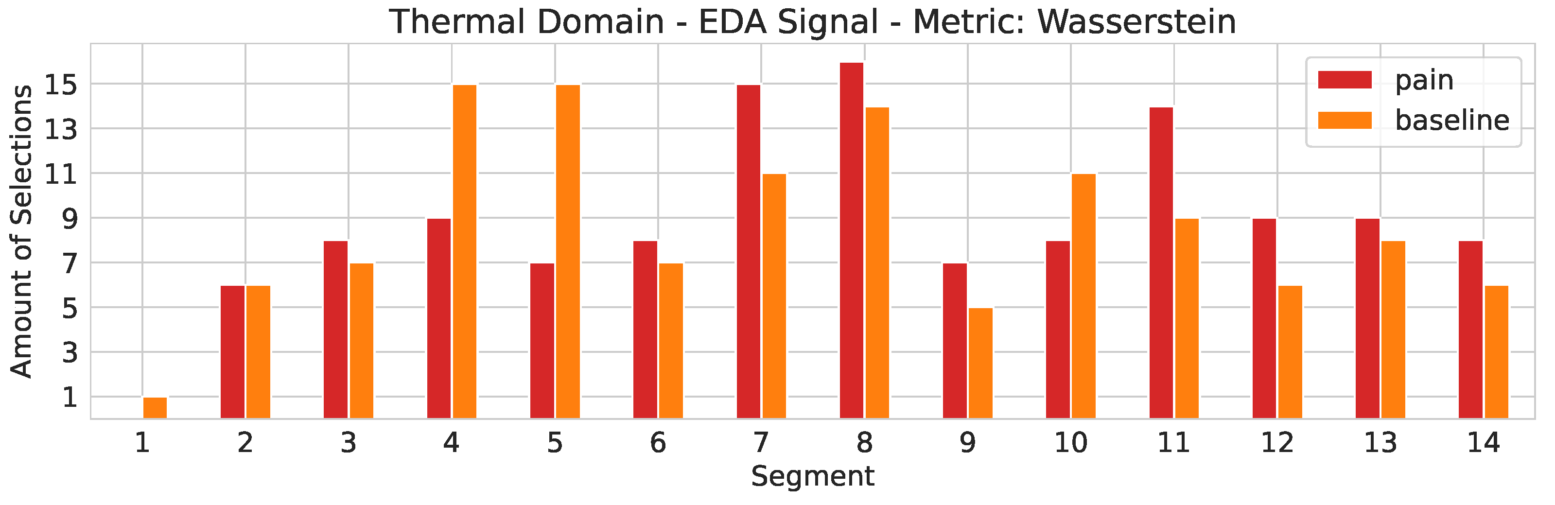
Figure 8.
Thermal domain. The segment selection frequency for the EDA signal in combination with the Wasserstein metric. On the x-axis the segment number is depicted. The y-axis represents the segment counter.
Figure 8.
Thermal domain. The segment selection frequency for the EDA signal in combination with the Wasserstein metric. On the x-axis the segment number is depicted. The y-axis represents the segment counter.
Table 1.
Number of features per single- and multi-modality. Corrugator (COR), Trapezius (TRA) and Zygomaticus (ZYG) are electromyogram (EMG) signals. ECG denotes the electrocardiogram, EDA denotes the electrodermal activity and EMG denotes the early fusion of COR, TRA, and ZYG. EFU denotes the early fusion over all modalities.
| ECG | EDA | COR | TRA | ZYG | EMG | EFU |
|---|
| 87 | 79 | 82 | 82 | 82 | 246 | 412 |
Table 2.
Label distribution per pain domain. PB: phasic baseline stimuli (no pain), PP: phasic pain stimuli, TB: tonic baseline stimuli (no pain), TP: tonic pain stimuli.
Table 2.
Label distribution per pain domain. PB: phasic baseline stimuli (no pain), PP: phasic pain stimuli, TB: tonic baseline stimuli (no pain), TP: tonic pain stimuli.
| Thermal Domain | Electric Domain |
|---|
| PB | PP | TB | TP | PB | PP | TB | TP |
| 3727 | 3716 | 121 | 124 | 3720 | 3719 | 123 | 123 |
Table 3.
Electric domain: Evaluation of the individual segments of the tonic samples based on uni- and multi-modal signals. Parameter k-S specifies the evaluated segment. NA: Naive approach, in which the model is trained on phasic stimuli and evaluated on the unmodified tonic samples (no segmentation). Ref.: Reference values obtained in the tonic domain. The LOSO-CV accuracies are given in %. The segment leading to the best outcome is depicted in bold, respectively.
| k-S | 1 | 2 | 3 | 4 | 5 | 6 | 7 | 8 | 9 | 10 | 11 | 12 | 13 | 14 | NA | Ref. |
|---|
| ECG | | | | | | | | | | | | | | | | |
| EDA | | | | | | | | | | | | | | | | |
| EMG | | | | | | | | | | | | | | | | |
| COR | | | | | | | | | | | | | | | | |
| TRA | | | | | | | | | | | | | | | | |
| ZYG | | | | | | | | | | | | | | | | |
| EFU | | | | | | | | | | | | | | | | |
Table 4.
Electro: Transfer from phasic to tonic stimuli. Evaluation of various distance metrics used to determine the closest segment. k-S: The highest accuracy value obtained in combination with the evaluation of the individual segments. NA: Naive approach in which the model is trained on phasic stimuli and evaluated on the unmodified tonic samples (no segmentation). Ref.: Reference values obtained in the tonic domain. The LOSO-CV accuracies are given in %. The metric leading to the best outcome is depicted in bold, respectively.
| Metric | Euclidean | City-Block | Chebyshev | Canberra | Bray-Curtis | Wasserstein | Hausdorff | k-S | NA | Ref. |
|---|
| ECG | | | | | | | | | | |
| EDA | | | | | | | | | | |
| EMG | | | | | | | | | | |
| COR | | | | | | | | | | |
| TRA | | | | | | | | | | |
| ZYG | | | | | | | | | | |
| EFU | | | | | | | | | | |
Table 5.
Electro: Transfer from phasic to tonic stimuli—Jensen–Shannon. Grid search over the bandwidth values for the kernel density estimation. k-S: The highest accuracy value obtained in combination with the evaluation of the individual segments. NA: Naive approach in which the model is trained on phasic stimuli and evaluated on the unmodified tonic samples (no segmentation). Ref.: Reference values obtained in the tonic domain. The LOSO-CV accuracies are given in %. The -value leading to the best outcome is depicted in bold, respectively.
| | | | | | | | k-S | NA | Ref. |
|---|
| ECG | | | | | | | | | | |
| EDA | | | | | | | | | | |
| EMG | | | | | | | | | | |
| COR | | | | | | | | | | |
| TRA | | | | | | | | | | |
| ZYG | | | | | | | | | | |
| EFU | | | | | | | | | | |
Table 6.
Thermal domain: Evaluation of the individual segments of the tonic samples in combination with the uni- and multi-modal signals. Parameter k-S specifies the evaluated segment. NA: Naive approach in which the model is trained on phasic stimuli and evaluated on the unmodified tonic samples (no segmentation). Ref.: Reference values obtained in the tonic domain. The LOSO-CV accuracies are given in %. The segment leading to the best outcome is depicted in bold, respectively.
| k-S | 1 | 2 | 3 | 4 | 5 | 6 | 7 | 8 | 9 | 10 | 11 | 12 | 13 | 14 | NA | Ref. |
|---|
| ECG | | | | | | | | | | | | | | | | |
| EDA | | | | | | | | | | | | | | | | |
| EMG | | | | | | | | | | | | | | | | |
| COR | | | | | | | | | | | | | | | | |
| TRA | | | | | | | | | | | | | | | | |
| ZYG | | | | | | | | | | | | | | | | |
| EFU | | | | | | | | | | | | | | | | |
Table 7.
Thermal domain: Transfer from phasic to tonic stimuli. Evaluation of various distance metrics used to determine the closest segment. k-S: The highest accuracy value obtained in combination with the evaluation of the individual segments. NA: Naive approach in which the model is trained on phasic stimuli and evaluated on the unmodified tonic samples (no segmentation). Ref.: Reference values obtained in the tonic domain. The LOSO-CV accuracies are given in %. The metric leading to the best outcome is depicted in bold, respectively.
| Metric | Euclidean | City-Block | Chebyshev | Canberra | Bray-Curtis | Wasserstein | Hausdorff | k-S | NA | Ref. |
|---|
| ECG | | | | | | | | | | |
| EDA | | | | | | | | | | |
| EMG | | | | | | | | | | |
| COR | | | | | | | | | | |
| TRA | | | | | | | | | | |
| ZYG | | | | | | | | | | |
| EFU | | | | | | | | | | |
Table 8.
Thermal domain: Transfer from phasic to tonic stimuli—Jensen–Shannon. Grid search over the bandwidth values for the kernel density estimation. k-S: The highest obtained accuracy value in combination with the evaluation of individual segments. NA: Naive approach in which the model is trained on phasic stimuli and evaluated on the unmodified (no segmentation) tonic samples, Ref.: Reference values obtained in the tonic domain. The LOSO-CV results are given in %. The -value leading to the best outcome is depicted in bold, respectively.
| | | | | | | | k-S | NA | Ref. |
|---|
| ECG | | | | | | | | | | |
| EDA | | | | | | | | | | |
| EMG | | | | | | | | | | |
| COR | | | | | | | | | | |
| TRA | | | | | | | | | | |
| ZYG | | | | | | | | | | |
| EFU | | | | | | | | | | |


