1. Introduction
The scientific study of traffic flow began in the 1930s with the implementation of the probabilistic theory for describing vehicular traffic jointly with the research undertaken by Bruce D. Greenshields at the Yale Highway Traffic Bureau, including employed research on traffic’s behavior when having intersections and integrating volume and speed models [
1]. The rise of automobile usage and the increase in highway systems that took place after World War II were boosters that escalated the analysis of traffic characteristics and theories about traffic flow. Therefore, the 1950s represents advancements of theoretical developments from diverse approaches, including motorcar tracking [
1].
There are different microscopic models representing different tasks or problems that a car faces during its travel; one approach is vehicle tracking models. There are also lane change models to determine the decision of a driver to change lanes or not during his trip. Usually, through a logical sequence of questions, these models are capable of making decisions based on the desired speed of the car and the situation of the preceding one, inducing a lane change when there are gaps between the circulating cars and allowing a safe maneuver [
2,
3].
There are also gap acceptance models to represent the decisions faced by a driver when choosing to maneuver at a priority intersection or in the process of changing lanes. Vehicle tracking models, which correspond to the best-known microscopic models, are those that show the tracking of a car, usually limited by the preceding automobile; therefore these models correspond to a set of equations to determine how each car performs its tracking, taking into account the behavior of the preceding vehicle [
3,
4]. There are different approaches to model the path traveled by one car when following another. There are approaches where the model seeks to establish that the driving response is proportional to the stimulus that an individual or a car may receive. In the case of the vehicle following model, braking or acceleration is taken as the response to a stimulus, which corresponds to the difference in relative speed between two cars and their corresponding relative distance, i.e., the difference in speeds of the leading and the following car over the difference in relative distance of the car in front and the one behind multiplied by a parameter that relates the driver’s own characteristics (fatigue, sleep, distractions, sight-hearing, mood, alcohol, cell phone use, smoking, GPS, drugs, medication, stress, depression, habits, skill, and caution) as well as some characteristics of the environment (road conditions, weather, road lighting), which influence the driver’s behavior [
5,
6].
By representing each car with its own equation that defines its progress, among other factors, microscopic models require significant computational power to be solved. Currently, there are a number of computational packages that solve these models by simulation with a user interface known as “micro traffic simulators”, and although some of them are intended for purely academic use, most of them are commercial products used in consulting. A relevant consideration when using these micro-simulators is their adaptability to the local conditions where they are to be implemented. It is important to emphasize that the fact that they are models with a high level of detail does not imply that their power or capacity to replicate reality is high or better than that of macroscopic models [
7,
8,
9]. How appropriate one model or the other is will depend on what is sought with the modeling. In many cases, simplicity, in terms of the parameters to be calibrated and accuracy of the macroscopic models, is an important factor to be considered. In any case, it should always be kept in mind that these models are only a simplified representation of reality and that there is no perfect model [
7,
8,
9].
According to [
5], “social effects” are scarcely portrayed as models in the description of microscopic driving conducts in terms of driver’s decisions while driving. Nevertheless, a vehicle’s social effect interactions can be compiled when compared to other vehicles to see the affectations in the driver’s behaviors when, for instance, such interactions are the consequence of imitating other drivers. Thus, instant response behavior is influenced by both peer drivers and the social environment.
Regarding driving style, the way a driver performs is a complex issue that depends on different factors, such as psychophysical characteristics, as well as the type of vehicle used and the characteristics of the road [
10]. Several investigations have considered factors such as knowledge, mental state, and physical conditions, among others. A parameter regarded as significant is the reaction time for defensive maneuvers (obstacle avoidance and braking) [
11]. In this way, an important aspect is the hand-eye coordination of the driver, which may be subject to visibility (illumination), which may depend on the time of day, the proper functioning of the vehicle’s lights, or even related eye diseases. Factors of influence may include exhaustion of the driver and stress, among other aspects [
12].
Regarding a related work, in [
13], a review on the incorporation of human factors in car-following models is carried out. Particularly, [
5] inquires into the empirically evident existence of the social effect when a faster vehicle overtakes the other under consideration, determining if the driver displays any form of imitation regarding the overtaker vehicle. The gathered information refers to 63 host vehicles by checking on accelerations, positions, and velocities, with specific information of the environment in a frequency of 10 Hz. Additionally, the authors included models to draw heterogeneity in the observations to examine positive and negative variations in the social effect using “logit” models. Consequently, the resulting outcomes showed that drivers display identical behaviors to the passing vehicles.
Another related work can be seen in [
14], where a five-parameter social force car tracking model was established. When it comes to studying well-founded alternatives to solve the issue of vehicle trajectories, the authors determined a hysteresis with clockwise and counterclockwise movement according to the model parameters. The model was also capable of reproducing waves intermittently to periods and amplitudes according to field observations when combining stochastic vehicle dynamics in the trajectory of the leading vehicle. In addition, such a model is suitable to generate waves intermittently to periods and amplitudes according to field observations when combining stochastic vehicle dynamics.
1.1. Traffic Models at the Microscopic Level
The method of replication of traffic scenarios is extensively employed in researching systems and networks of traffic and developments and planning alike. Currently, literary sources offer numerous schemes of traffic simulations in the realm of experimentation, aiming to measure operations in real traffic. Such traffic scenarios can be divided as microscopic modeling, macroscopic modeling, and mesoscopic modeling [
15]. Microscopic traffic modeling analyzes each car individually and investigates the relationships between them.
Calibration is needed in microscopic traffic simulations in models of vehicle displacement or car tracking [
16]. During various driving conditions, control parameters in such models include the time interval, an individual driver’s space, and acceleration. Recently, those parameters have been defined for different types of vehicles and estimated from macroscopic data flow such as volume and average speed. Notwithstanding, such data are incapable of determining real behaviors in individual vehicles, and the impact of the first vehicle class on the next vehicle’s behavior is disregarded in the estimation of parameters. Considering the above, the authors in [
16] estimated the parameters associated with driving behavior for heavy vehicles and cars in the classical Wiedemann model for vehicle following.
A variation of this type of model can be seen in [
17], where a model containing spring block chain asymmetric interactions is taken as the starting point to an ideal single-lane road traffic flow. Thus, primary elements encompass static and kinetic friction, namely drivers and cars’ inertia, the spatiotemporal disorder prompted by the values in these forces of friction (driving demeanors), blocks (automobiles), and unidirectional interactions with springs (this refers to keeping a distance from fellow drivers).
An approach to analyzing the behavior in individual car-following is attempted in [
18] by applying the stimulus-response concept. In this scenario, the researchers suggested a model of safety, defined as the anticipated level of risk in the processes of cars following other cars. Then, the evaluation of acceleration takes place regarding the difference between the desired safety margin (or acceptable risk level) and the perceived risk level (or perceived safety margin).
On the other hand, in [
19], the authors posited that the correlation between the expected time interval and the time of speed adaptation sets the arrangement formation in jammed traffic flow. Thus, such associations exert control over individual and collective responses of vehicles in traffic.
Another work can be seen in [
20], where a model was used to establish the effect of vehicular technology in terms of energy consumption and consequent emissions. Sustainable development requires, among other things, reducing both energy usage and pollutant emissions caused by traffic. The researchers considered affectations that emanated from energy consumption and emissions as a result of transport hybridization in road traffic (single lanes).
A work where vehicle combinations are incorporated into stimulus-response automobile following models can be seen in [
21]. The authors used separate models to determine responses regarding acceleration and deceleration in vehicle combinations across various states of motion and vehicle types. For various pairs of following vehicles, each model integrated three sub-models, including scenarios such as a truck following a car, a car following a truck, and a car following another car. According to the results, the behaviors of drivers were considerably different regarding different pairs of vehicles.
According to [
22], traditional methods for identifying historical crash data are strongly considered to identify high-risk locations. Conventional safety metrics, such as time to collision, ignore the risks associated with scenarios of car following. In particular, in cases when the speed of the follower vehicle is almost the same as that of the leading vehicle and the space in between them is moderately small, a slight perturbation of the collision risk is produced. To address this limitation, the authors in [
22] proposed time to collision with perturbations for risk identification. By means of a hypothetical perturbation, measurements assessed rear-end conflict risk in car-following scenarios, including ones with a higher speed of the leading vehicle.
Finally, in [
23], to study possible relationships of leading and following vehicle, the authors proposed a car-tracking model that combines a convolutional neural network (CNN) with a long short-term memory (LSTM) network. For this model, 400 car tracking periods were taken from the OpenACC car tracking experiment database and a natural driving database. The CNN is used to extract the features of the car-tracking behavior, while the LSTM network using the feature vector is used to anticipate the acceleration of the follower vehicle.
1.2. Traffic Models with Driver Behavior
According to [
24], driving behavior models are a relevant aspect of road traffic simulation modeling. Features such as reaction, tiredness, and mood in distracting conditions can be considered. Models should consider associations between a driver’s performance and external factors. In this regard, a methodology for the establishment of driver behavior model parameters was proposed in [
24]. The proposal is based on traffic data to generate the car-tracking model and thus establish the parameters that best represent driving habits.
Considering that driver’s behavior characteristics (DBC) influence car-following safety, reference [
25] analyzed the effect of different DBC as a function of the desired safety margin (DSM), which includes five DBC parameters. The study shows that higher risk perception levels can reduce RECs (rear-end collisions); a faster driver reaction capability can avoid RECs, and higher deceleration sensitivity can improve car-following safety.
According to [
26], intense congestion, traffic crashes, and discomfort often occur on uneven pavements due to imperfect decisions made by human drivers. Autonomous vehicles (AV) are an alternative to improve driving performance and replace human driving. In this regard, Ref. [
26] recommends an approach employing intelligent speed control for autonomous cars by using deep reinforcement learning (DRL) to acquire behaviors of following a safe car based on information regarding the road and traffic, aiming at safety improvements, driving comfort, and efficiency.
On the other hand, in [
27], a test scenario design method considering real longitudinal characteristics was proposed for the verification of Autonomous Driving Systems (ADS) and Advanced Driver Assistance Systems (ADAS). The recommended method comports a model that imitates vehicle behavior including an additional model of driver in response to different driving environments. Such model employs the Model Predictive Control (MPC) algorithm for emulating similar features in human driving. The lengthwise driver’s features were acquired from a database analysis of large-scale driving.
According to [
28], as the supply of vehicles with autonomous driving functions increases, vehicle safety also becomes an emerging problem; therefore, the authors in [
28] used a camera with a variable focus function to ensure safety when applying the RSS (responsibility-sensitive safety) model. In this way, an improved RSS model was proposed, taking into account changing road conditions due to weather, which is a factor that promotes safe distance between cars.
1.3. Focus and Organization of the Article
Considering that mobility is an important factor for the quality of life of citizens, this paper aims to characterize the behavior of drivers. Such behavior in traffic models is a complex issue that addresses many aspects and can be approached in different ways. To this end, a fuzzy logic system is proposed to model driver’s behavior incorporated into the dynamic vehicle tracking model. Real data obtained from vehicle speed measurements on several urban roads are used to adjust the model.
This article does not consider the driver’s own characteristics due to the limitations that this represents for its measurement. The work takes into account the characteristics of the environment that are common to drivers, such as the state of the road, traffic, and lighting. The proposed fuzzy logic model seeks to incorporate these aspects in order to characterize the behavior of drivers subject to these factors.
At the simulation level, more real models can be implemented when including factors that affect drivers, allowing to propose traffic control strategies effective in real scenarios (applications).
The data needed to optimize the fuzzy logic model correspond to the speed of each car, so that when simulating the traffic model, the purpose is to obtain the same speed of the measured vehicles. Thus, different scenarios are considered to perform the optimization of the fuzzy logic model in order to characterize the behavior of drivers in different scenarios.
The simulation model allows us to establish the speed of the vehicles and their relationship with the parameter associated with the acceleration in such a way that the speed of the simulated vehicles is close to the real data. The data with which the fuzzy logic model is adjusted and validated were taken from various urban locations, where the factors that externally influence drivers include the level of lighting (day or night), road conditions (good or bad), and congestion (high or low). It should also be noted that single-lane sectors were considered, given the characteristics of the traffic model employed.
The paper is organized as follows.
Section 2 describes the vehicle tracking system model, and the fuzzy logic system model is presented in
Section 3. The process to perform the parameter optimization of the fuzzy logic system is described in
Section 4. The way the data were collected is presented in
Section 5; these data were used for the fuzzy logic system adjustment, and the results of this process are described in
Section 6. Finally, the discussion and conclusions of this work are presented in
Section 7 and
Section 8.
2. Dynamic Vehicle Tracking Model
Traffic simulation is mostly applied in researching traffic networks and systems related to planning and development. According to literary sources, various models are determined when studying real traffic operations. Traffic simulation models can be classified into three areas: microscopic modeling, macroscopic modeling, and mesoscopic modeling. In the microscopic traffic model, each car is analyzed individually, and the relationships between them are investigated. In reviews of these models, a general description of traffic simulation models is made in [
15] in terms of function, limitation, and application. Moreover, reference [
29] revises micro-simulations of various car tracking models and tools for autonomous and human driving behavior. Another review of these models is done in [
30] on simulation schemes under conditions of mixed traffic framing simulations and car-tracking models. The model considered in this work consists of a one-way tracking scheme, such as those presented in [
31,
32,
33,
34].
Considering a line of vehicles, all of length
L and equal mass, as shown in
Figure 1, since there is only one line of traffic, there are no overtakings, and the positions
…
. Thus, the spacing between vehicles
i and
is given by:
The separation given in Equation (
1) will change if the speed of the leading vehicle changes, where
m is the respective mass. Considering that the
i-th vehicle has a braking force
, the deceleration of the vehicle is given by:
The braking force depends on the speed and the relative distance of the vehicle
i with respect to the vehicle in front,
; in this way, the braking force can be written as:
where
A is a parameter that relates the characteristics of the driver (habits, knowledge, ability, caution
…) as well as the characteristics of the environment (holes, level of vision, rain…). In this way, we can obtain:
Considering that the right-hand side of Equation (
4) can be represented as the derivative of a logarithm, then, we can obtain:
Thus, we establish Equation (
6), where
is a factor that depends on the initial conditions.
It should be noted that this expression is not valid for
since the leading vehicle does not have another vehicle in front.
Figure 2 shows the block diagram for the simulation of the model for a leading and a follower vehicle. In this figure,
is the respective velocity
associated with the leading vehicle, and
is the factor related to the driver’s skill and habits.
In this way, the set of differential equations that describes the system in
Figure 2 is the following:
3. Fuzzy Logic Model
The models of fuzzy logic portrays fuzzy sets associated with information (concepts) combined between inputs and outputs to form rules for setting outputs [
35,
36]. Fuzzy systems allow the modeling of nonlinear processes and also receive inputs from a dataset employing learning (optimization) algorithms. Systems based on fuzzy logic endow easy use of preliminary knowledge as an initial point for optimization [
37]. In fuzzy rule-based systems, the connections between variables are characterized as follows:
A characteristic of
X is named a linguistic label and is featured by a fuzzy set in the universe of discourse
X. One of the most-used fuzzy logic models corresponds to the Mamdani type, where fuzzy sets are used in the antecedent and in the consequent to represent concepts associated with the input and output variables. In this way, the rules are obtained through the relation of the fuzzy sets of the inputs and the outputs [
35,
36].
This work seeks to characterize the behavior of drivers by measuring the speed of vehicles, since mobility is an important factor for the quality of life of citizens. A fuzzy logic system is employed to model the driver’s behavior, which is incorporated into the dynamic vehicle tracking model, whose adjustment is made using real data measured on urban roads. The model disregards characteristics of the driver due to existing limitations for measuring the physical and psychological conditions of each driver. The model includes characteristics of the environment common to drivers, such as the state of the road, lighting, and the state of congestion.
The fuzzy logic model considers common parameters to all drivers, that is, environmental instead of personal conditions. Thus, the input variables are:
Light: This is considered if there is natural or artificial lighting (day or night).
Traffic: This variable considers whether there is a slow or fast flow of vehicles due to the time of day (rush hour).
Road: This refers to the quality of the road on which the vehicle circulates (adequate or poor lane conditions).
The output variable of the model corresponds to the parameter
K in the vehicle tracking model.
Figure 3 shows the fuzzy logic model where inputs and output are presented.
The Mamdani-type fuzzy logic system is used to ensure the interpretability of the fuzzy sets associated with the inputs and the output. In this way, after performing the optimization process, linguistic labels (concepts) can be assigned to the fuzzy sets associated with the output.
Sigmoidal functions are used in the fuzzy system, such as those shown in
Figure 4, which are used to represent high and low values on a scale from 0 to 1 for each of the input variables. Equation (
10) corresponds to the sigmoidal function, where
is associated with the width of the transition area, and
is the center of the transition area.
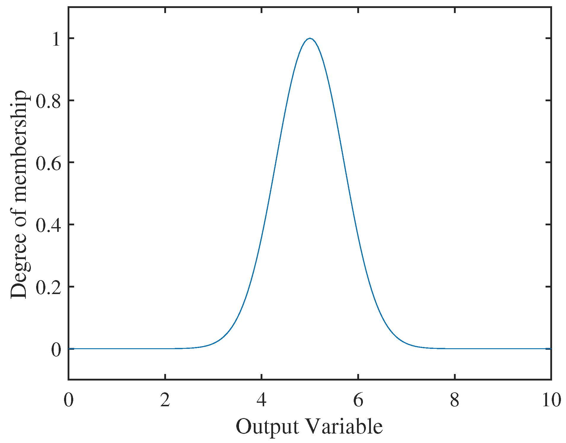
In addition, Gaussian sets are used for the output;
Figure 5 shows the shape of one of the fuzzy sets. Equation (
11) corresponds to the Gaussian function, where
is the standard deviation and
is the mean.
The rules correspond to the combination of all input sets having an associated output fuzzy set. In this way, the set of rules can be seen in
Table 1. It is noticeable that more fuzzy sets can be used to consider more input features; however, the number of cases and, therefore, the measurements to be carried out increase. It is worth noting that the output fuzzy sets do not have associated concepts or linguistic labels, which can be established after the optimization process.
4. Model Fitting Process through Optimization
Considering that an initial configuration of the fuzzy system can be determined, then to perform the adjustment of this system can employ an optimization algorithm that uses this initial configuration as the starting point. Additionally, in this case, when using Gaussian functions, there are no constraints on the parameters of the sets, so an algorithm without restrictions can be used.
In an unconstrained optimization algorithm, to determine the next point in an iteration, there are two strategies: line search and confidence region. In the line search strategy, a direction is chosen in which a point that provides a lower value of the objective function is searched, and in each iteration, a new direction and a new point are searched. In the trusted region strategy, a model function is constructed that approximates the objective function; since the model for certain points differs from the objective function, a region is established where this approximation is suitable, which is called the confidence region [
38].
An example of an algorithm with a line search strategy is the quasi-Newton method, where successive approximations of the Hessian are performed. Examples of methods based on trust regions are those that use quadratic forms [
38].
When the function is to be minimized (with several variables), Newton’s method uses the Equation (
12), where
f is the function to minimize,
X is the vector composed by the variables of
f, where
is the vector of the first derivative of
f, which is also called a gradient, and finally,
is the Hessian matrix, where the respective elements correspond to the second derivatives of
f.
For implementing the quasi-Newton method, successive approximations of the Hessian inverse are made since the calculation of this inverse can be expensive from the computational point of view. This set of methods is called quasi-Newtonian, and it includes the Davidon–Fletcher–Powell (DFP) method, which performs successive approximations of the inverse of the Hessian, and the Broyden–Fletcher–Goldfarb–Shannon (BFGS) method, where the Hessian is approximated [
38].
Fitness Function
The fitness function (objective function) used for the adjustment of the fuzzy system corresponds to the mean squared error (MSE) given by Equation (
13), where
J corresponds to the objective function,
X is the set of parameters (associated with the model),
n is the index associated to the discrete time,
r is the actual measured data (on the roads),
s is the data calculated from the model simulation, and
N is the total amount of data taken.
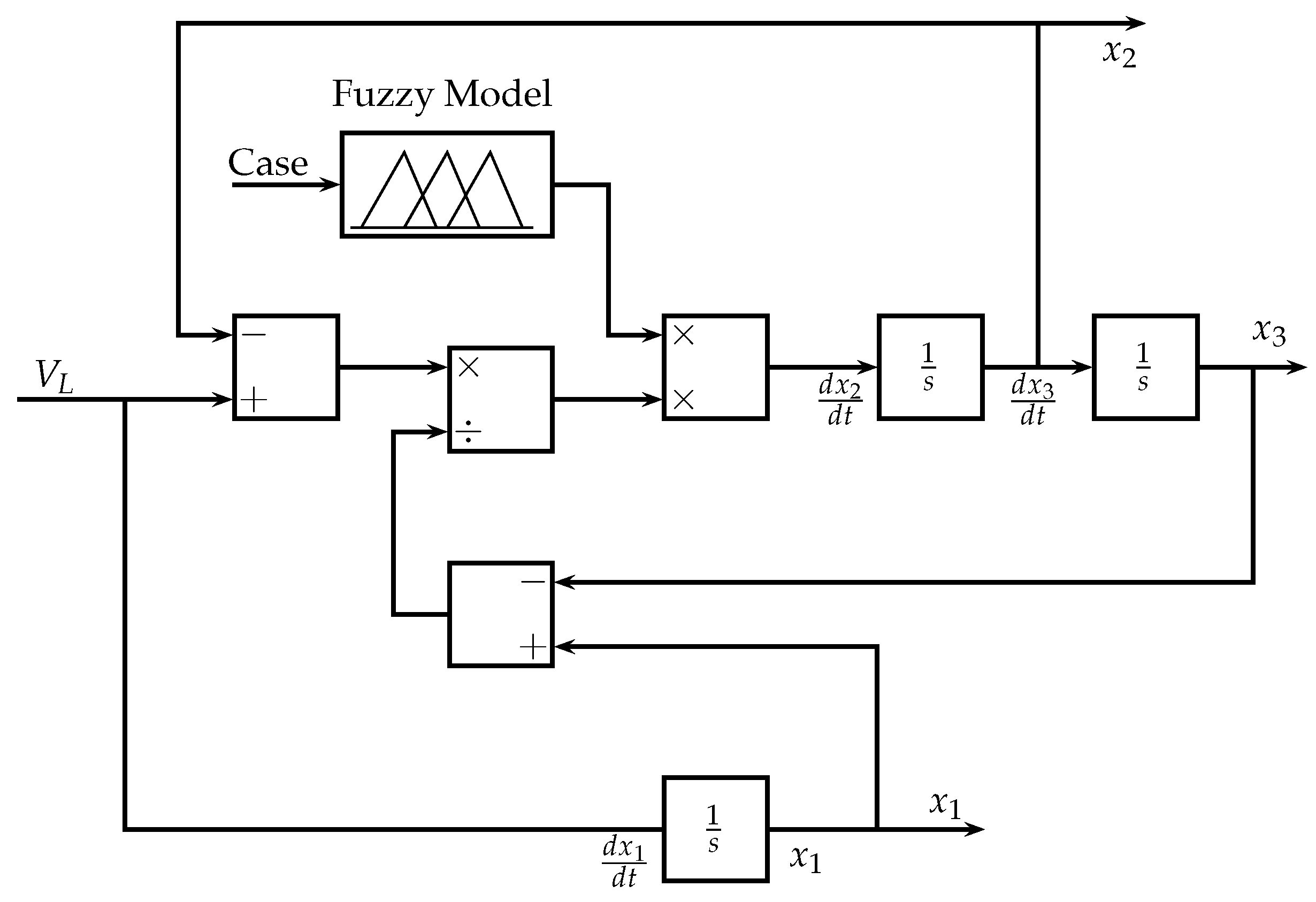
Figure 6 shows the block diagram for the simulation of the model considered to perform the optimization of the fuzzy system. In this scheme,
is the respective velocity associated with the leading vehicle. The input of the fuzzy model corresponds to the case of the environmental factors that affect drivers.
In
Figure 6, the input of the fuzzy system (Case) corresponds to the coding of each case in such a way that the fuzzy inference process delivers the respective factor associated with the driving factor. In this way, during the optimization process, each case is evaluated, and the simulation result is contrasted with the real data in a way that the adjustment of the fuzzy logic system is achieved.
5. Data Used
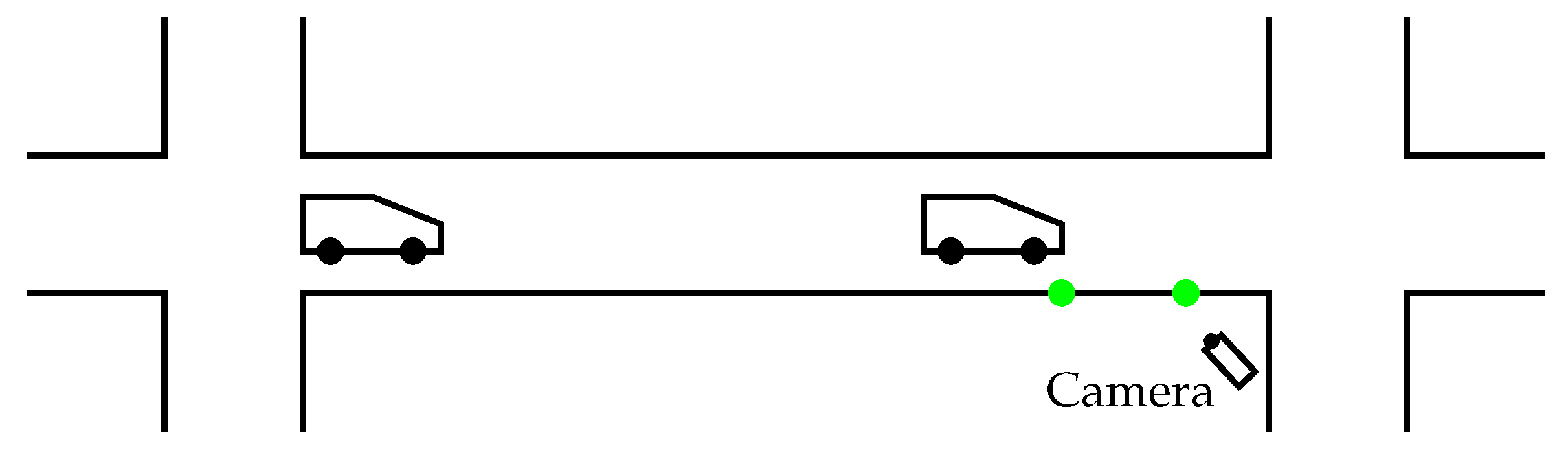
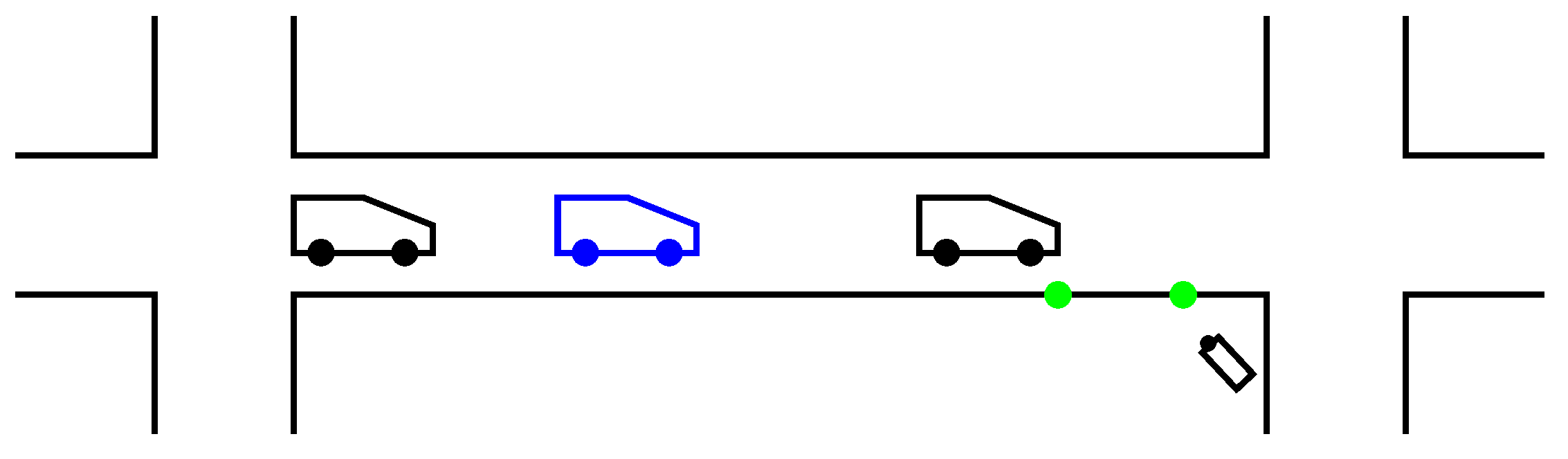
As displayed in
Table 1, eight different scenarios are considered for data collection, for which the setup shown in
Figure 7 is used, where a camera is used to measure the displacement and velocity of vehicles at the end of the block. It should be noted that the distance between the green marks is 12 m. The camera features are the following:
Model: Sony hdrcx305e;
Image device: size 4.5 mm (1/4 type) EXMOR R CMOS Sensor;
Shutter speed: 1/8–1/1000 (including scene selection);
Number of pixels, gross (K): 4200;
Clearvid technology: Yes;
Image processor: BIONZ;
Telemacro: Yes;
X.V. Colour: Yes;
Steadyshot (image stabilisation): Optical SteadyShot Active Mode;
Minimm illumination (lux): 3 lux (1/25 shutter speed);
Number of pixels by camera mode(K): 16:9 mode, 2650, 4:3 mode, 1990, 16:9 mode, 2650, 4:3 mode, 3540;
White balance: Auto/outdoor/indoor/one-push;
Backlight compensation: Yes;
Camera noise reduction: Yes.
The data collection was carried out in different places of Zipaquirá, a municipality of the department of Cundinamarca, Colombia.
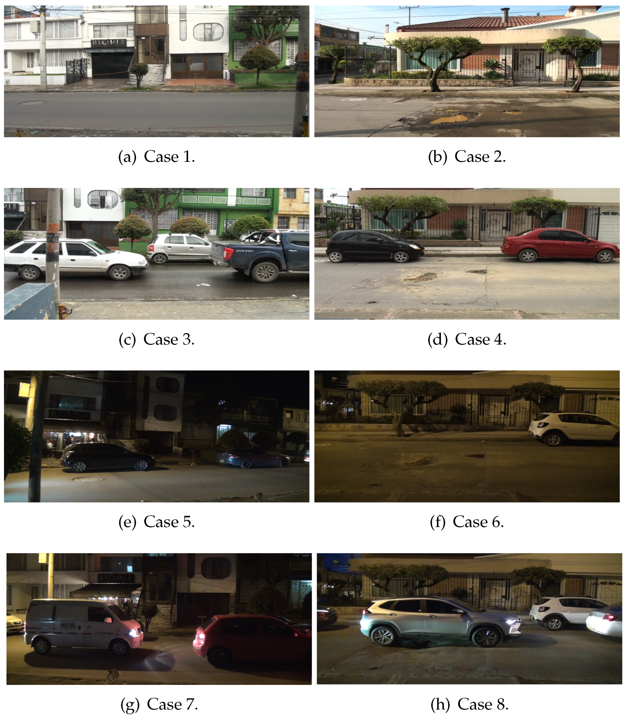
Table 2 shows the characteristics and location of the places where the data were measured. Meanwhile,
Figure 8 shows the roads and the cases considered, where most cases involved straight roads with a low volume of vehicular flow; these aspects were considered to facilitate data collection and model adjustment. It should be noted that for cases 2, 4, 6, and 8, the pictures were taken to show one of the visible deteriorations of the road, and its location is different from the one used to make the measurements.
In this way, for each scenario, the data acquisition was carried out for approximately one hour, and the speeds of the vehicles were measured at the end of the block.
Table 3 shows the statistical summary of the measured data having the samples, maximum, minimum, average, and standard deviation (STD). It is worth noting that in case 7, there are only 102 measurements since it was necessary to stop the data collection for security reasons. It should be noted that the time is given in seconds
s, the distance in meters
m, and the speed in meters per second m/s.
6. Results
In order to fit (train) the fuzzy logic system, of the data were used for optimization, and were used for testing. The codification for the input variables was made considering the following values:
Light: Day = 1, and Night = 0.
Traffic: High = 1, and Low = 0.
Road: Good = 1, and Bad = 0.
The optimization variables correspond to the parameters of the fuzzy sets associated with the output variable. Since the cases for the input variables are well established in
Table 1, parameter optimization for the sets associated with the input variables was not performed.
Considering Equation (
11), the initial configuration of the fuzzy sets for the output variable
y corresponds to a location of its mean value at
with a variance of
. The optimization process was performed on a Lenovo PC IdeaPad 5 14ITL05 with an 11th Gen Intel Core i7-1165G7 processor 2.80 GHz, with 16.0 GB of RAM. In this order, performing the optimization process, the run time was 2904.91 s. The MSE values obtained before and after the optimization process for both the test and training data can be seen in
Table 4.
Given the limitations in data collection, the concept of a virtual vehicle was utilized to implement the model, which serves as the leader of the vehicle under consideration in such a way that at the end of the simulation, it is sought that the vehicle reaches the same speed of the leading vehicle (virtual), which can be seen in blue in
Figure 9. Since there is no dataset that allows a direct comparison with the vehicle tracking model, the virtual vehicle concept allows each vehicle to be considered separately and thus is able to carry out the optimization process of the fuzzy logic system incorporated into the traffic model.
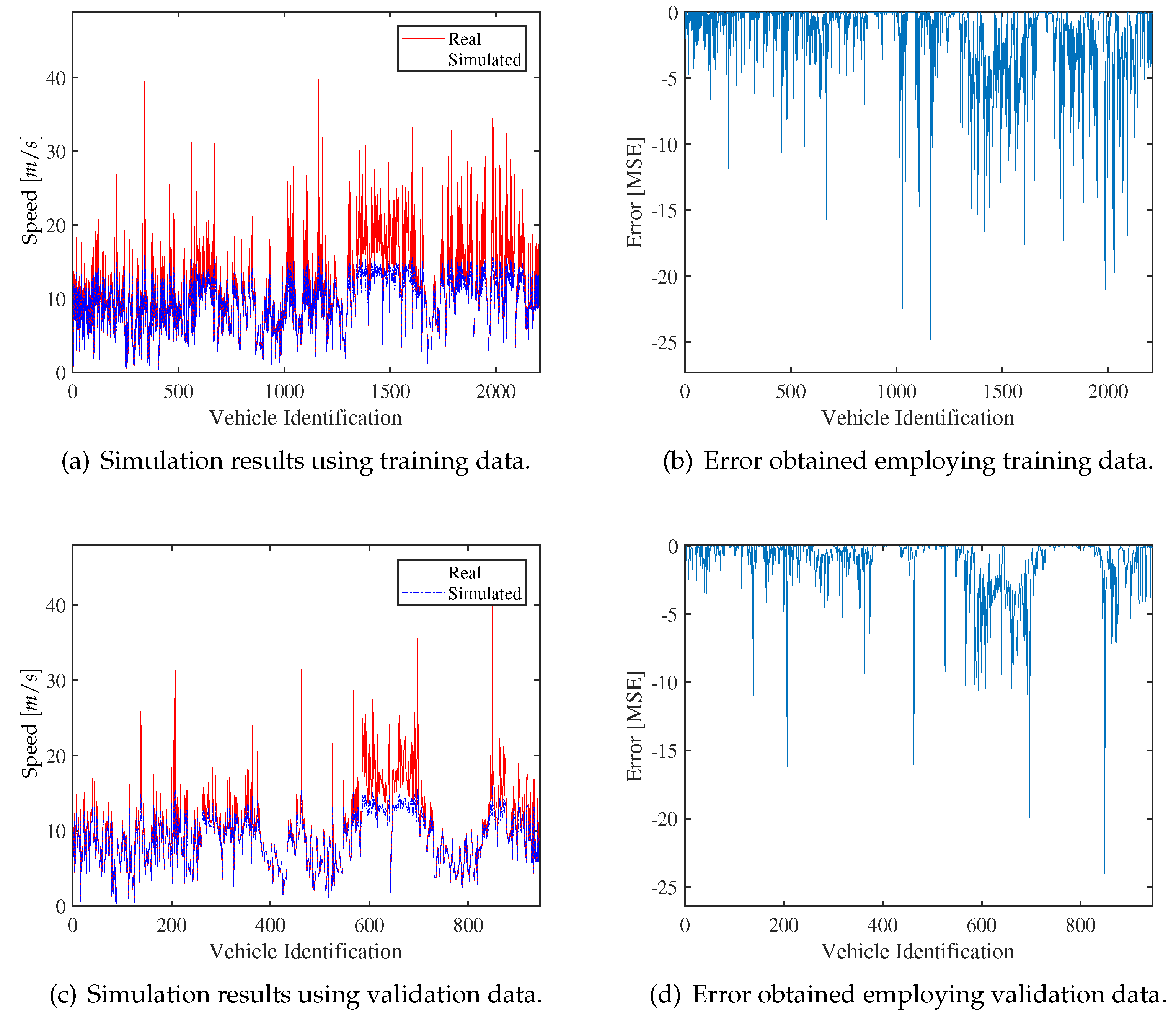
As a first result,
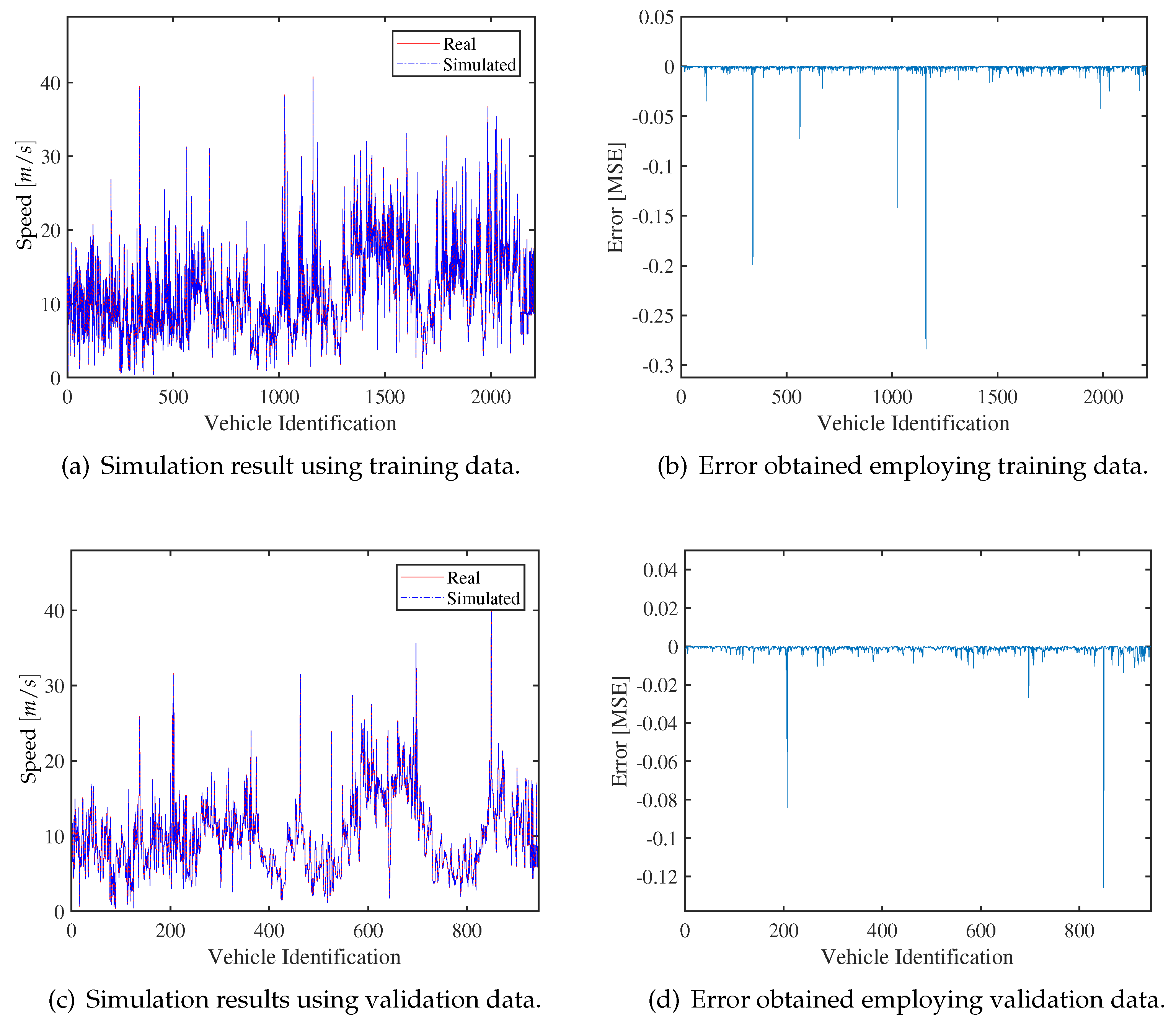
Figure 10 shows the model simulation without performing the optimization process, that is, with the rules obtained in a preliminary way. Meanwhile,
Figure 11 shows the simulation with the fuzzy system after the optimization process, where the simulated data are close to the real data. It is noteworthy that the training data and the test (validation) data are employed to evaluate the fuzzy model before and after optimization. These figures also display the error value obtained for each measurement using the training and validation data.
Before the optimization process, in
Figure 10a,c, we can observe the difference between the real and simulated data. After the optimization process, in
Figure 11a,c the simulated data are close to the real data.
Meanwhile, in
Figure 10b,d and
Figure 11b,d the error displays only negative values, which is consistent with the model since it is considered that the follower vehicle does not outperform the leading vehicle.
As observed in
Figure 10, although the values of the velocities obtained with the model differ from the real measurements, the model generates values close to the real data, which shows that the initial configuration of the fuzzy system allows the adjustment of the model using the quasi-Newton method.
In these results, it is also observed that the values obtained with the validation data are similar (or better) in comparison with those obtained with the test data, which shows that overtraining does not occur.
From
Figure 10, which was obtained using training and test data before the optimization process, it is observed that the largest errors occur for high values of speed.
It is also worth noting that, after the optimization process,
Figure 11b,d displays some high error values, which is mainly observed when having high speeds that may be related to the inaccuracy in the speed measurement process.
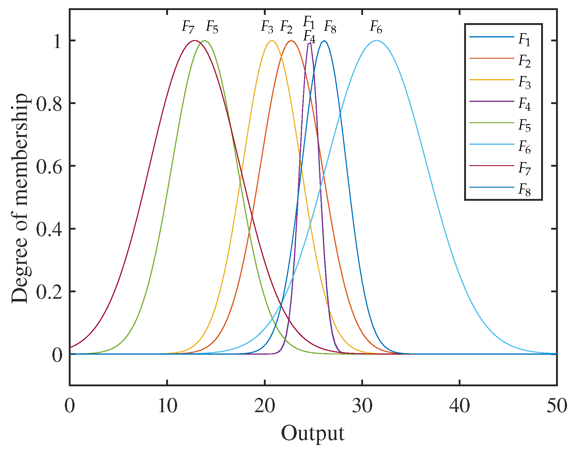
A remarkable result for the interpretability of the fuzzy system is the location of the consequent sets, as seen in
Figure 12. In this way, considering the values of the output variable, it is possible to assign linguistic labels (concepts) to the output fuzzy sets.
Regarding the interpretability of the fuzzy logic system, in
Figure 12, it can be seen that sets
and
are located in the same place with the same amplitude, and that set
was associated with low values and
was associated with high values. The intermediate (half) values were associated with
,
,
,
, and
. It is also noteworthy that the highest variance is presented by
, followed by
, and the lowest variance is presented by
and
. Considering these results, it is possible to assign linguistic labels for the output sets, obtaining the tags shown in
Table 5. These labels allow a linguistic relationship between the input variables (environment factors) and the action that the driver would take for the different scenarios considered.
7. Discussion
For the development of this work, different limitations were presented from the data acquisition to the design of the fuzzy logic system and the traffic model implementation.
Firstly, there is a limitation in data collection since an interval of 12 m was considered to measure the average speed of the vehicle at the end of the street (considering vehicles of the same length). Only the movement of vehicles in a single lane was taken into account; therefore, the behavior of drivers when overtaking was not modeled. Additionally, data were only taken for certain urban sectors, which adjust to the characteristics of the traffic model used.
Secondly, the fuzzy logic model considers environmental factors common to all drivers since a particular study of each driver is beyond the scope of this work. Therefore, the model obtained allows for an average characterization of drivers. There is also a limitation in the number of fuzzy sets used to model each of the concepts associated with each input and output of the system.
Thirdly, for the integration of the traffic model with the fuzzy logic model and the optimization process, it was necessary to include the concept of virtual vehicles since there is no detailed dataset for a direct comparison with the traffic model. The virtual vehicle concept allows each vehicle to be considered separately and thus is able to carry out the optimization process of the fuzzy logic system.
Despite the limitations that arose in the development of this work, adequate optimization of the fuzzy logic system was achieved, obtaining an adequate interpretability of this since the location of the fuzzy sets in the universe of output discourse represents the actions that would be taken by a conductor depending on the characteristics considered. Given the limitations that this work presented, it can be considered as a first approximation to model the behavior of drivers using a fuzzy model. This research can serve as a reference mark for developing computational traffic models considering aspects that affect the behavior of drivers.
A Mamdani-type fuzzy logic system was proposed to ensure the interpretability of the fuzzy sets associated with the inputs and output. After performing the optimization process, linguistic labels (concepts) can be associated with the fuzzy sets of the output. This turns out to be an alternative to incorporate into the traffic model factors that affect drivers.
This model can be extended by considering other traffic scenarios, as well as other types of driver behaviors and different roads. It can also be improved by using a larger and more detailed dataset; for a better comparison with other schemes, a greater number of data can be acquired, which is outside the scope of this work and can therefore be developed in the future.
8. Conclusions
A fuzzy logic model was proposed that relates the behavior of drivers, considering their driving style and taking into account different factors that are external to the driver. In the implementation, different limitations were presented from the data acquisition, the design of the fuzzy logic system and the implementation of the traffic model. Despite these limitations, adequate optimization of the fuzzy logic model was achieved.
The dynamic car-following model, through the optimization process and using the real data measured in different urban sectors, allows the optimization of the proposed fuzzy logic system to characterize driver’s behavior. The optimization process could be improved by using a larger and more detailed dataset. Therefore, future work in this area should focus on expanding the available datasets, incorporating more scenarios to further refine the model and increase its applicability in real-world situations.
Fuzzy logic systems can be used to model the behavior of drivers on urban roads by considering different environmental factors. The incorporation of a fuzzy logic system into a dynamic vehicle tracking model allows the inclusion of driver’s behavior. The use of fuzzy logic in the optimization process helped to fine-tune the model and improve its accuracy.
After carrying out the optimization process, it was possible to assign linguistic labels to the fuzzy sets associated with the output discourse universe. In this way, the interpretability of the proposed fuzzy system is achieved by assigning labels (concepts) to the fuzzy sets.
The initial configuration of the fuzzy system allowed us to implement the optimization process using the quasi-Newton method, which requires an initial search point.
Regarding future works, it is possible to improve the model considering other scenarios, such as the inclusion of overtakings and other driver behaviors. This allows creating a more comprehensive and accurate representation of real-world driving conditions. This could enhance the applicability of the fuzzy logic model in practical transportation planning and traffic engineering applications. In addition, another focus should be based on collecting a larger and more detailed dataset to further optimize the proposed fuzzy logic model, particularly in relation to driver behavior in different urban sectors.
To increase the interpretability of the model, a future work could explore alternative methods for assigning linguistic labels to the fuzzy sets, such as incorporating expert input or using natural language processing techniques.
Author Contributions
Conceptualization, L.A.B., H.E.E. and C.E.M.; Methodology, L.A.B., H.E.E. and C.E.M.; Project administration, L.A.B., H.E.E. and C.E.M.; Supervision, H.E.E.; Validation, C.E.M.; Writing—original draft, L.A.B., H.E.E. and C.E.M.; Writing—review and editing, L.A.B., H.E.E. and C.E.M. All authors have read and agreed to the published version of the manuscript.
Funding
This research received no external funding.
Institutional Review Board Statement
In this work, direct tests were not carried out on individuals (humans).
Informed Consent Statement
The data were taken from vehicle measurements.
Data Availability Statement
The data used can be requested from the authors.
Acknowledgments
The authors express their gratitude to the Universidad Distrital Francisco José de Caldas. We also give special recognition to Joaquín Javier Meza Álvarez.
Conflicts of Interest
The authors declare no conflict of interest.
References
- Gartner, N.H.; Messer, C.; Rathi, A. Traffic Flow Theory—A State-of-the-Art Report: Revised Monograph on Traffic Flow Theory; Organized by the Committee on Traffic Flow Theory and Characteristics (AHB45); Turner-Fairbank Highway Research Center: McLean, VA, USA, 2002. [Google Scholar]
- Mahmud, S.M.S.; Ferreira, L.; Hoque, S.; Tavassoli, A. Micro-simulation modelling for traffic safety: A review and potential application to heterogeneous traffic environment. IATSS Res. 2019, 43, 27–36. [Google Scholar] [CrossRef]
- Yi, Z.; Lu, W.; Qu, X.; Gan, J.; Li, L.; Ran, B. A bidirectional car-following model considering distance balance between adjacent vehicles. Phys. A Stat. Mech. Its Appl. 2022, 603, 127606. [Google Scholar] [CrossRef]
- Yuan, Z.; Wang, T.; Zhang, J.; Li, S. Influences of dynamic safe headway on car-following behavior. Phys. A Stat. Mech. Its Appl. 2022, 591, 126697. [Google Scholar] [CrossRef]
- Mohammadi, S.; Arvin, R.; Khattak, A.J.; Chakraborty, S. The role of drivers’ social interactions in their driving behavior: Empirical evidence and implications for car-following and traffic flow. Transp. Res. Part F Traffic Psychol. Behav. 2021, 80, 203–217. [Google Scholar] [CrossRef]
- Wen, X.; Cui, Z.; Jiana, S. Characterizing car-following behaviors of human drivers when following automated vehicles using the real-world dataset Author links open overlay panel. Accid. Anal. Prev. 2022, 172, 106689. [Google Scholar] [CrossRef]
- Amini, E.; Tabibi, M.; Khansari, E.R.; Abhari, M. A vehicle type-based approach to model car following behaviors in simulation programs (case study: Car-motorcycle following behavior). IATSS Res. 2019, 43, 14–20. [Google Scholar] [CrossRef]
- Ci, Y.; Wu, L.; Zhao, J.; Sun, Y.; Zhang, G. V2I-based car-following modeling and simulation of signalized intersection. Phys. A Stat. Mech. Its Appl. 2019, 525, 672–679. [Google Scholar] [CrossRef]
- Mai, M.; Wang, L.; Prokop, G. Advancement of the car following model of Wiedemann on lower velocity ranges for urban traffic simulation. Transp. Res. Part F Traffic Psychol. Behav. 2019, 61, 30–37. [Google Scholar] [CrossRef]
- Jurecki, R.S.; Stanczyk, T.L.; Ziubinski, M. Analysis of the Structure of Driver Maneuvers in Different Road Conditions. Energies 2022, 15, 7073. [Google Scholar] [CrossRef]
- Benderius, O.; Markkula, G.; Wolff, K.; Wahde, M. Driver behaviour in unexpected critical events and in repeated exposures—A comparison. Eur. Transp. Res. Rev. 2013, 6, 51–60. [Google Scholar] [CrossRef] [Green Version]
- Jurecki, R.S. Influence of the Scenario Complexity and the Lighting Conditions on the Driver Behaviour in a Car-Following Situation. Arch. Automot. Eng.-Arch. Motoryz. 2019, 83, 151–173. [Google Scholar] [CrossRef]
- Saifuzzaman, M.; Zheng, Z. Incorporating human-factors in car-following models: A review of recent developments and research needs. Transp. Res. Part C Emerg. Technol. 2014, 48, 379–403. [Google Scholar] [CrossRef] [Green Version]
- Delpiano, R.; Laval, J.; Coeymans, J.E.; Herrera, J.C. The kinematic wave model with finite decelerations: A social force car-following model approximation. Transp. Res. Part B Methodol. 2015, 71, 182–193. [Google Scholar] [CrossRef]
- Nor-Azlan, N.N.; Md-Rohani, M. Overview of Application of Traffic Simulation Model. MATEC 2018, 150, 03006. [Google Scholar] [CrossRef] [Green Version]
- Durrani, U.; Lee, C.; Maoh, H. Calibrating the Wiedemann’s vehicle-following model using mixed vehicle-pair interactions. Transp. Res. Part C Emerg. Technol. 2016, 67, 227–242. [Google Scholar] [CrossRef]
- Járai-Szabó, F.; Sándor, B.; Néda, Z. Spring-block model for a single-lane highway traffic. Cent. Eur. J. Phys. 2011, 9, 1002–1009. [Google Scholar] [CrossRef] [Green Version]
- Lu, G.; Cheng, B.; Wang, Y.; Lin, Q. A Car-Following Model Based on Quantified Homeostatic Risk Perception. Math. Probl. Eng. 2013, 2013, 408756. [Google Scholar] [CrossRef] [Green Version]
- Birlea, N.M. Shaping traffic flow with a ratio of time constants. Cent. Eur. J. Eng. 2014, 4, 155–161. [Google Scholar] [CrossRef]
- Boubaker, S.; Rehimi, F.; Kalboussi, A. Effect of vehicular technology on energy consumption and emissions. Int. J. Environ. Stud. 2015, 72, 667–684. [Google Scholar] [CrossRef]
- Siuhi, S.; Kaseko, M. Incorporating vehicle mix in stimulus-response car-following models. J. Traffic Transp. Eng. 2016, 3, 226–235. [Google Scholar] [CrossRef] [Green Version]
- Xie, K.; Yang, D.; Ozbay, K.; Yang, H. Use of real-world connected vehicle data in identifying high-risk locations based on a new surrogate safety measure. Accid. Anal. Prev. 2019, 125, 311–319. [Google Scholar] [CrossRef] [PubMed]
- Qin, P.; Li, H.; Li, Z.; Guan, W.; He, Y. A CNN-LSTM Car-Following Model Considering Generalization Ability. Sensors 2023, 23, 660. [Google Scholar] [CrossRef] [PubMed]
- Mecheva, T.; Furnadzhiev, R.; Kakanakov, N. Modeling Driver Behavior in Road Traffic Simulation. Sensors 2022, 22, 9801. [Google Scholar] [CrossRef] [PubMed]
- Zhang, J.; Yang, C.; Zhang, J.; Ji, H. Effect of Five Driver’s Behavior Characteristics on Car-Following Safety. Int. J. Environ. Res. Public Health 2023, 20, 76. [Google Scholar] [CrossRef] [PubMed]
- Chen, J.; Zhao, C.; Jiang, S.; Zhang, X.; Li, Z.; Du, Y. Safe, Efficient, and Comfortable Autonomous Driving Based on Cooperative Vehicle Infrastructure System. Int. J. Environ. Res. Public Health 2023, 20, 893. [Google Scholar] [CrossRef]
- Cho, K.; Park, C.; Lee, H. A Study on Longitudinal Motion Scenario Design for Verification of Advanced Driver Assistance Systems and Autonomous Driving Systems. Appl. Sci. 2023, 13, 716. [Google Scholar] [CrossRef]
- Kim, M.J.; Kim, Y.M. RSS Model Improvement Considering Road Conditions for the Application of a Variable Focus Function Camera. Sensors 2023, 23, 592. [Google Scholar] [CrossRef]
- Ahmed, H.U.; Huang, Y.; Lu, P. A Review of Car-Following Models and Modeling Tools for Human and Autonomous-Ready Driving Behaviors in Micro-Simulation. Smart Cities 2021, 4, 314–335. [Google Scholar] [CrossRef]
- Matcha, B.N.; Namasivayam, S.N.; Fouladi, M.H.; Ng, K.C.; Sivanesan, S.; Eh-Noum, S.Y. Simulation Strategies for Mixed Traffic Conditions: A Review of Car-Following Models and Simulation Frameworks. J. Eng. 2020, 2020, 8231930. [Google Scholar] [CrossRef] [Green Version]
- Pignataro, L.J.; Cantilli, E.J. Traffic Engineering: Theory and Practice; Prentice-Hall: Englewoods Cliffs, NJ, USA, 1973. [Google Scholar]
- Bender, E.A. An Introduction to Mathematical Modeling; Dover Publications INC: New York, NY, USA, 1978. [Google Scholar]
- Lieu, H. Traffic-Flow Theory A State-of-the-Art Report; AHB45; Committee on Traffic Flow Theory and Characteristics: Amsterdam, The Netherlands, 2001. [Google Scholar]
- Lia, C.; Jianga, X.; Wanga, W.; Chenga, Q.; Shen, Y. A Simplified Car-Following Model Based on the Artificial Potential Field. Procedia Eng. 2016, 137, 13–20. [Google Scholar] [CrossRef] [Green Version]
- Peckol, J.K. Introduction to Fuzzy Logic; John Wiley & Sons: Hoboken, NJ, USA, 2021. [Google Scholar]
- Espitia, H.; Soriano, J.; Machón, I.; López, H. Design Methodology for the Implementation of Fuzzy Inference Systems Based on Boolean Relations. Electronics 2019, 8, 1243. [Google Scholar] [CrossRef] [Green Version]
- Sadollah, A. Fuzzy Logic Based in Optimization Methods and Control Systems and Its Applications; IntechOpen: London, UK, 2018. [Google Scholar]
- Xue, D. Solving Optimization Problems with MATLAB®; De Gruyter: Berlin, Germany; Boston, MA, USA, 2020. [Google Scholar]
Figure 1.
Diagram of vehicles in a lane, all of length L and equal mass. The spacing will change if the speed of the vehicle ahead changes.
Figure 1.
Diagram of vehicles in a lane, all of length L and equal mass. The spacing will change if the speed of the vehicle ahead changes.
Figure 2.
Block diagram of the leader-follower model, where is associated with the leading vehicle, and K is the factor related to the driver’s skill.
Figure 2.
Block diagram of the leader-follower model, where is associated with the leading vehicle, and K is the factor related to the driver’s skill.
Figure 3.
Fuzzy logic model with eight rules, where the input variables are the light, the traffic, and the road. The output corresponds to the driving factor in the vehicle tracking model.
Figure 3.
Fuzzy logic model with eight rules, where the input variables are the light, the traffic, and the road. The output corresponds to the driving factor in the vehicle tracking model.
Figure 4.
Fuzzy sets used for input variables representing high and low membership values.
Figure 4.
Fuzzy sets used for input variables representing high and low membership values.
Figure 5.
Fuzzy sets used for the output variable (Gaussian membership function).
Figure 5.
Fuzzy sets used for the output variable (Gaussian membership function).
Figure 6.
Block diagram of the traffic model incorporating the fuzzy system. The input of the fuzzy model corresponds to the case of the environmental factors that affect drivers.
Figure 6.
Block diagram of the traffic model incorporating the fuzzy system. The input of the fuzzy model corresponds to the case of the environmental factors that affect drivers.
Figure 7.
Setup for data acquisition. The camera was used to measure displacement and velocity of vehicles after taking the respective videos.
Figure 7.
Setup for data acquisition. The camera was used to measure displacement and velocity of vehicles after taking the respective videos.
Figure 8.
Pictures of the places where the data were collected in Zipaquirá, municipality of the department of Cundinamarca, Colombia.
Figure 8.
Pictures of the places where the data were collected in Zipaquirá, municipality of the department of Cundinamarca, Colombia.
Figure 9.
Representation of the virtual vehicle in blue, which serves as the leader of each real vehicle.
Figure 9.
Representation of the virtual vehicle in blue, which serves as the leader of each real vehicle.
Figure 10.
Results obtained from the model simulation before the optimization process.
Figure 10.
Results obtained from the model simulation before the optimization process.
Figure 11.
Results obtained from the model simulation after the optimization process.
Figure 11.
Results obtained from the model simulation after the optimization process.
Figure 12.
Optimized output fuzzy sets, where we can observe the location and shape of each membership, making it possible to assign a linguistic label to each set.
Figure 12.
Optimized output fuzzy sets, where we can observe the location and shape of each membership, making it possible to assign a linguistic label to each set.
Table 1.
Fuzzy rule set.
| Light | Traffic | Road | Output |
|---|
| Day | Low | Good | |
| Day | Low | Bad | |
| Day | High | Good | |
| Day | High | Bad | |
| Night | Low | Good | |
| Night | Low | Bad | |
| Night | High | Good | |
| Night | High | Bad | |
Table 2.
Location of the places for data collection in Zipaquirá, municipality of the department of Cundinamarca, Colombia.
Table 2.
Location of the places for data collection in Zipaquirá, municipality of the department of Cundinamarca, Colombia.
| Case | Light | Traffic | Road | Location |
|---|
| Case 1 | Day | Low | Good | 11th Avenue, between 5th and 6th Streets |
| Case 2 | Day | Low | Bad | 7th Street, between 10th and 11th Avenues |
| Case 3 | Day | High | Good | 11th Avenue, between 5th and 6th Streets |
| Case 4 | Day | High | Bad | 7th Street, between 10th and 11th Avenues |
| Case 5 | Night | Low | Good | 11th Avenue, between 5th and 6th Streets |
| Case 6 | Night | Low | Bad | 7th Street, between 10th and 11th Avenues |
| Case 7 | Night | High | Good | 11 Avenue, between 5th and 6th Streets |
| Case 8 | Night | High | Bad | 7th Street, between 10th and 11th Avenues |
Table 3.
Statistical summary of the measured data.
Table 3.
Statistical summary of the measured data.
| Case | Case 1 | Case 2 | Case 3 | Case 4 | Case 5 | Case 6 | Case 7 | Case 8 |
|---|
| Samples | 314 | 435 | 251 | 641 | 268 | 403 | 102 | 739 |
| Max | 39.4737 | 31.0912 | 31.6288 | 40.797 | 20.7479 | 33.1783 | 18.7702 | 39.9614 |
| Min | 0.3702 | 2.4534 | 2.9811 | 0.9871 | 0.6165 | 1.7455 | 4.3573 | 1.2157 |
| Average | 8.1643 | 10.6249 | 9.2037 | 8.9577 | 9.5345 | 17.4148 | 10.2832 | 12.4063 |
| STD | 4.7555 | 4.014 | 4.5172 | 4.9869 | 3.7045 | 4.6925 | 4.0437 | 5.9195 |
Table 4.
MSE values before and after optimization.
Table 4.
MSE values before and after optimization.
| Data | Before Optimization | After Optimization |
|---|
| Training | | |
| Test | | |
Table 5.
Linguistic labels for the output sets.
Table 5.
Linguistic labels for the output sets.
| Light | Traffic | Road | Output |
|---|
| Day | Low | Good | : Half High |
| Day | Low | Bad | : Half |
| Day | High | Good | : Half Low |
| Day | High | Bad | : Half High |
| Night | Low | Good | : Low |
| Night | Low | Bad | : Very High |
| Night | High | Good | : Very Low |
| Night | High | Bad | : High |
| Disclaimer/Publisher’s Note: The statements, opinions and data contained in all publications are solely those of the individual author(s) and contributor(s) and not of MDPI and/or the editor(s). MDPI and/or the editor(s) disclaim responsibility for any injury to people or property resulting from any ideas, methods, instructions or products referred to in the content. |
© 2023 by the authors. Licensee MDPI, Basel, Switzerland. This article is an open access article distributed under the terms and conditions of the Creative Commons Attribution (CC BY) license (https://creativecommons.org/licenses/by/4.0/).


