Article

Benefits of Using Network Modeling Platforms When Studying IP Networks and Traffic Characterization

Faculty of Engineering, South-West University “Neofit Rilski”, 2700 Blagoevgrad, Bulgaria
Computers 2023, 12(2), 41; https://doi.org/10.3390/computers12020041
Submission received: 8 January 2023 / Revised: 11 February 2023 / Accepted: 13 February 2023 / Published: 16 February 2023

Abstract

:
This article addresses the benefits of using IP network modeling platforms to study IP networks. For the purposes of this study, several models of IP networks were created, through which various hypotheses were studied. Additionally, different operational variants of the modeled IP networks were created. The use of the GNS3 platform was proposed, as well as several tools for monitoring the processes in IP networks. The application of IP network modeling platforms to study power electronic devices was also addressed. IP network modeling platforms greatly facilitate both the process of studying IP networks and the process of training professionals to design, install, and maintain different types of IP network. Thanks to the GNS3 IP network modeling platform, it was possible to implement different models of IP networks with different functionalities. It was very easy to determine the answers to posed hypotheses/questions through the capabilities of the IP network modeling platforms. The questions posed by the hypotheses addressed in this paper were answered thanks to the results obtained from the research carried out with the IP network modeling platform GNS3. The present study confirmed that the use of these platforms, in particular the GNS3 platform, for the modeling of IP networks is an excellent substitute for expensive network equipment, and the IP network models created in the platform performed almost like networks made of real devices.

1. Introduction

In the last decade, IP technology has established total hegemony over the communication network field. Other communication technologies have been displaced by this technology, which has even taken hold in the new generation of mobile communications—4G and 5G. Every single device, regardless of whether it is used in the household or in industry, must already have the ability to connect to an IP network—wired or wireless. Thanks to IP technology, people’s lives around the world have been completely changed, for better or for worse. In addition, users are constantly provided with new services and opportunities, such as 4K IPTV, VoIP (voice over IP), VOLTE (voice over LTE), and Vo5G (voice over 5G). In order for these services to be provided to users, it is necessary to train specialists who can maintain and develop IP technology and, accordingly, IP networks. In order to be perfectly prepared, these specialists need to be trained and familiarized with all possible practical situations. This is best achieved when working/learning with real network devices. The problem here is that not every educational institution, such as a high school or university, can afford to purchase professional, high-performance network equipment, as it is very expensive. In order to be able to train high-quality network specialists, regardless of the financial capabilities of the training institution, a convenient solution is the use of IP network modeling platforms.
The best way to solve the problem of not being able to use/purchase suitable network equipment is through the use of IP network modeling platforms. Using such platforms solves the abovementioned problems. The main disadvantage of using IP network modeling platforms is the need to use workstations with very high computing capabilities in order for the simulation/modeling to run smoothly. In the present work, the capabilities of such a platform (GNS3) for the modeling of IP networks are presented. The benefits of using IP network modeling platforms are discussed with several demonstrations of working IP network models. Through these examples, different IP networks were studied, presenting different functionalities, such as: connecting to other real networks (the Internet), VoIP services, and characterizing the communication traffic generated by power electronic devices (PEDs). Various IP network monitoring tools were used to study and monitor the modeled IP networks. Based on the obtained results, a brief analysis was conducted for each of the studied modeled IP networks.

2. Article Structure

This article has the following structure:
  • Section 1—Introduction. Here is presented a brief description of the state of the problem under consideration;
  • Section 2—structure of the article;
  • Section 3—Related work. Here is presented a review of various works related or very close to the problem discussed in this article;
  • Section 4—Used platform and additional tools. Here are explained the choice to use the GNS3 platform and the monitoring and measurement tools used during the study;
  • Section 5—Research methodology. Here is presented a brief explanation of how the research was carried out;
  • Section 6—Working models of experimental IP networks. Here, the studied models of IP networks are presented in detail, as well as the results obtained from the studies;
  • Section 7—Discussion and analysis of the obtained results;
  • Section 8—Conclusion.

3. Related Work

In Ref. [1], the authors used the modeled IP network to verify different transition techniques for carrying IPv4 packets through IPv6 packets. To carry out their research, the authors also used the Wireshark tool for monitoring IP networks. Thus, using GNS3, the authors could very easily verify how the proposed transition techniques handled the transfer of IPv4 packets through IPv6 packets without using real expensive network equipment. A similar study was conducted in [2,3,4].
In Ref. [5], the author used the capabilities of GNS3 to study, compare, and evaluate the possibilities of ensuring secure data exchange when applying the two protocols that are used to encrypt information when building VPN (Virtual Private Network) tunnels. The evaluation and comparison of the capabilities between the two protocols were again carried out using Wireshark. This author’s research once again demonstrated the many capabilities of IP network modeling platforms.
In Ref. [6], the author evaluated the performance of different routing protocols. The modeled IP network created therein was initially configured to work with only one protocol, then with the second protocol, and finally with the third protocol. The IP network model comprised nine routers. If such an experimental network were to be built with nine routers, it would be very expensive. Thanks to GNS3, there was no need to purchase these routers.
In Ref. [7], the author used another platform, Riverbed Modeler, to model any kind of communication network. The aim of the study was to verify the performance of the sensor network when using different numbers of nodes (from 3 to 40) and topologies. Such research without the help of a communication network modeling platform would be difficult to implement.
In Ref. [8], the authors compared the performance of OSPF (Open Shortest Path First for IPv4) and OSPFv3 (Open Shortest Path First for IPv6). Again, the Riverbed Modeler platform was used. To this end, the authors created a model of an IP network composed of several subnets, each with a certain number of devices. Two scenarios were modeled—one where the network operated only with OSPF, and a second where the network operated only with OSPFv3. Evidently, the use of a communication network modeling platform was necessary for this kind of research to be carried out. Without the use of such a platform, this research would be difficult or even impossible to realize due to the large number of network devices and nodes.
In Ref. [9], the authors used the capabilities of Riverbed Modeler to model an IP network that would be subjected to cyber-attacks. The aim of the work was to assess the results of a cyber-attack on the operability of an IP network with security policies applied. Thus, it was possible to study what would happen to the network before it was physically built and put into operation. This work showed another capability of communication network modeling platforms—the verification of the security level of a working network. This type of research would be difficult to implement without the availability of communication equipment. However, thanks to communication network modeling platforms, this type of research can easily be implemented. Additional studies similar to this work can be found in [10,11].
In Ref. [12], the authors modeled a VoIP network. The purpose of this work was to study and determine the values of various parameters affecting the performance of a VoIP network—the delay, bandwidth, jitter, packet size, packet loss, and others. This type of research—the quick assessment of certain parameters—is realized very rapidly only using communication network modeling platforms. Additional studies similar to the reviewed work can be found in [13,14].
In Ref. [15], the authors proposed an algorithm for protecting the exchange of service information used to identify the nodes, through blockchain technology, in a mobile ad-hoc network (MANET). The effectiveness of the proposed algorithm was verified by the creation of a model MANET network that was subjected to cyber-attacks. This work showed another possibility for communication network modeling platforms, namely application in the development and testing of new algorithms, protocols, and technologies to be subsequently used in physical networks. Other similar developments can be seen in [16,17,18,19,20,21,22,23].
In conclusion, platforms for modeling communication networks are generally an excellent substitute for real networks, which was made evident by the small selection of research by various authors presented and reviewed above (there are thousands of developments on the subject in databases worldwide). Communication network modeling platforms can also be used to develop new algorithms and technologies to improve the performance of communication networks.
In the present work, several working models of IP networks were reviewed. Through these working models, the advantages of using IP network modeling platforms were highlighted by exploring the different capabilities offered by the selected platform. The research, of course, also took into account the disadvantages of the considered platform.

4. Used Platform and Additional Tools

4.1. Chosen Modeling Platform

For the purposes of this paper, the GNS3 platform [24] was used. This platform was chosen because of the advantages it offers, such as:
  • Compatibility with the operating systems of real network devices from global manufacturers;
  • Integration with various IP network monitoring tools;
  • The ability to connect the modeled network to real IP networks or the Internet;
  • Being completely free.
GNS3 can emulate the operation of various network devices, such as routers and switches. For this purpose, the platform uses disk images of the real operating systems of network devices. These operating systems are loaded into and emulated by the platform. Thus, GNS3 enables network professionals and trainees to work with real network devices without the need to purchase expensive network equipment. Thanks to this functionality, IP networks can be modeled using emulated network devices from real manufacturers. Thus, the modeled networks can come very close to real networks built with the corresponding network devices.
Another functionality of the platform is its integration with other IP network monitoring tools. In this way, the modeled network can be monitored with various monitoring tools. GNS3 makes it possible to monitor all links in the modeled network, so all traffic in the modeled network is monitored. In this way, it is possible to obtain as much data as possible about the performance of the network. Thanks to this functionality, the complete characterization of the traffic in the modeled network can be achieved.
The ability to connect to other real networks makes it possible to check how the performance of the modeled IP network changes when connected to the Internet. This functionality of GNS3 enables researchers to first model, test, and connect an IP network to the Internet/another real IP network; then study how connecting the modeled network affects its performance; and finally progress to the physical building of the modeled IP network.
GNS3 is completely free, which sets it apart from other platforms. For other platforms, the basic package of the platform is free, but one must pay for the full set of functionalities. For example, to achieve integration with traffic monitoring tools costs so much, and to have the modeled network be able to connect to real networks/the Internet costs an additional price. GNS3 has no such features. Therefore, this platform is very suitable for use in educational organizations such as colleges or universities that do not have additional funds to purchase different licenses.

4.2. Additional Tools Applied

For the purposes of the present work, several additional tools were used, through which the characterization of the traffic and the study of the modeled IP networks’ performance as presented in this article were carried out. The tools used were: a round-trip delay meter, a network analyzer, and a network protocol analyzer.
The Colasoft ping tool [25] and Solarwinds TracerouteNG [26] were used to measure the two-way (round-trip) delay in the modeled networks. These two tools monitored the round-trip delay in the modeled networks and provided graphical results illustrating how the round-trip delay changed during the study.
The network analyzer used was the Capsa Free Network Analyzer [27]. This monitored various parameters, such as: generated traffic, most-used protocols, and traffic generated from ports. Through this information, one could determine, for example, the most-used protocol and the port through which the most traffic was generated for each modeled network. Thus, the expected behavior of the modeled network when, for example, it is physically implemented is made clear. For the purpose of this article, the information from the network analyzer was used to characterize the traffic in the studied model IP networks.
The network protocol analyzer used herein was Wireshark [28]. Thanks to its integration with GNS3, it could monitor/capture packets on all links in the modeled network. This was also carried out in the present research. Thus, at the end of the study, the information from Wireshark could be processed and analyzed by additional tools in order to obtain additional graphical data for the characterization of the traffic in the studied model IP networks.
In addition, mathematical distributions were obtained for the size and arrival times of the packets (the time delays between the packets) [29,30,31]. Thus, additional graphical results were obtained and used to evaluate the studied model IP networks.

5. Research Methodology

The research presented herein was divided into three substudies, in which several hypotheses were examined.
The first study examined the hypothesis of whether using MPLS (Multiprotocol Label Switching) technology with OSPF and EIGRP (Enhanced Interior Gateway Routing Protocol) would make any difference in the performance of the modeled network. To test this hypothesis, a model of an IP network that accessed various resources on the Internet was created. Initially, the network worked only with MPLS and EIGRP, and in the subsequent study, the same modeled network worked only with MPLS and OSPF. For both networks, a characterization of the traffic exchanged in the modeled networks was carried out using the tools described in Section 5.
The second study examines the hypothesis of whether using MPLS technology with OSPF and EIGRP would have any impact on the performance of a VoIP network. To test this hypothesis, a model of a VoIP network was created in which voice streams were exchanged between individual subscribers. The modeled network was again able to access resources on the Internet. Again, the modeled network initially operated only with MPLS and EIGRP, and in the subsequent study, the network operated only with MPLS and OSPF. For the two networks, a characterization of the exchanged traffic was carried out, as well as a detailed analysis of the individual voice streams that were exchanged between the subscribers in the modeled VoIP network. The two-way delay (round-trip delay) in the modeled networks was measured. Finally, an analysis was carried out by comparing the results obtained when using only MPLS and EIGRP and when using only MPLS and OSPF. The results used for benchmarking were obtained via the tools described in Section 5.
The last study tested several hypotheses. The first hypothesis was that power electronic devices (PEDs) generate very little or no traffic. The second hypothesis was that connecting PEDs to an already built and working IP network does not lead to a change in the performance of the IP network. To verify these hypotheses, a characterization of the traffic generated by a studied power electronic device was performed, as well as a characterization of the traffic in an IP network before and after its connection to a PED. Several models of IP networks were created to characterize the traffic. Furthermore, the security of the data exchange between the PED and the control center was studied, and if found unsecure, proposals for how to secure the data exchange were put forward. Some of the tools described in Section 5 were used to test the hypotheses and verify the secure of the data exchange.

6. Working Models of Experimental IP Networks

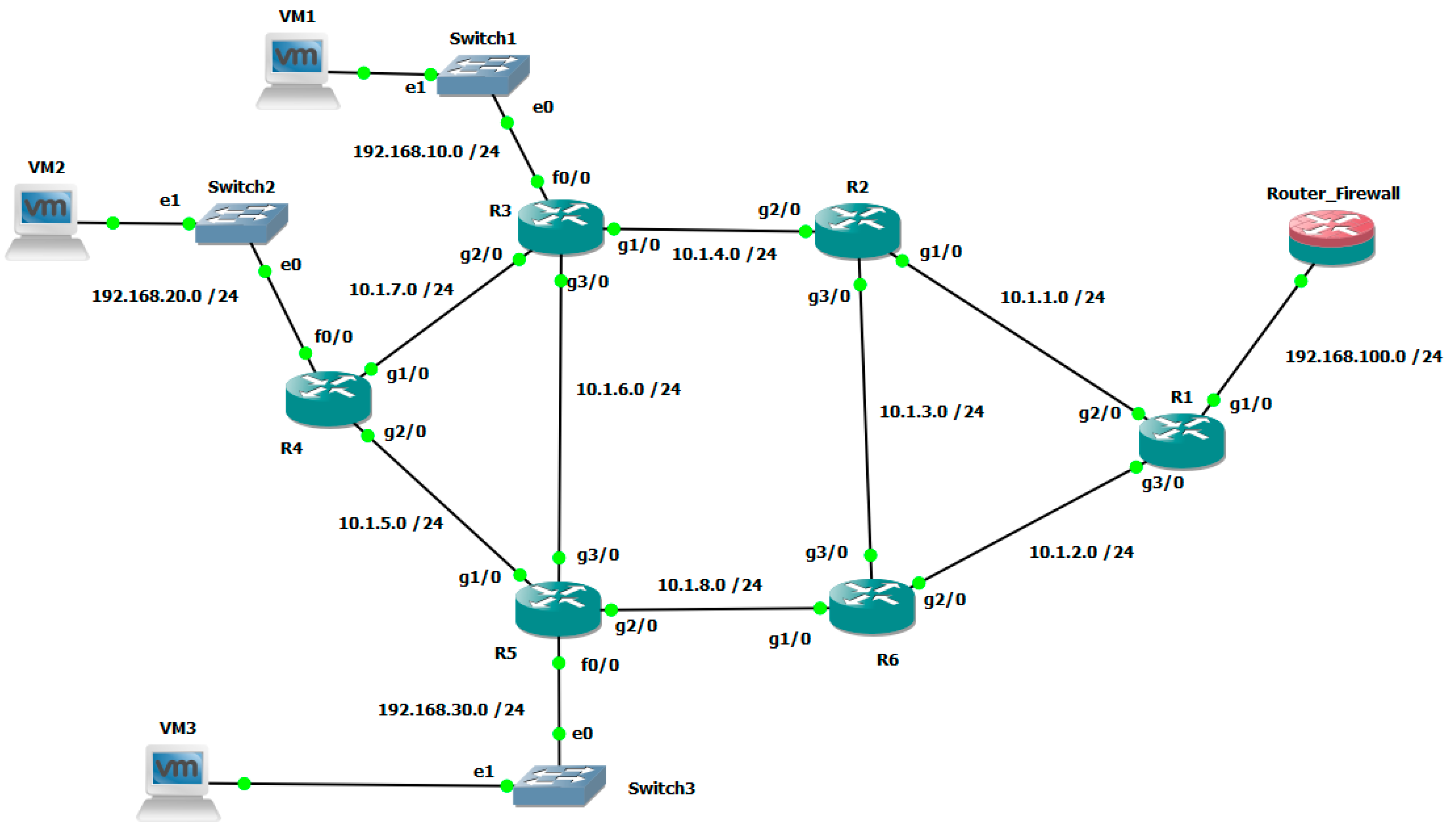
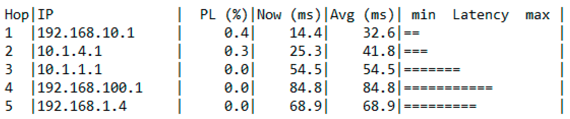
6.1. Model of IP Network Connected to the Internet

Figure 1 shows the topology of the modeled IP network. It consisted of six routers (R1 to R6) and three switches (Switch 1 to Switch 3), to which three virtual machines (VM1 to VM3) were connected, representing the users in the modeled network. Each of them accessed different resources on the Internet. VM1 accessed only one IP 4K CCTV (closed-circuit television) camera, VM2 accessed various YouTube channels, and VM3 was only used to download various files from the Internet. The modeled network showed the ability of GNS3 to connect to real IP networks; in this case, the modeled network was connected to the Internet. This was carried out through the Router_Firewall module, which acted as both a firewall and a border router, providing access to the Internet. The Router_Firewall module was created using the freeware pfSesne firewall [32]. In this scenario, two variants of the modeled network were studied. For the first variant, the network operated with EIGRP and MPLS, and for the second, it operated with OSPF and MPLS. The purpose of the research was to check if there was any difference when using MPLS technology with OSPF or EIGRP. To answer this question, a characterization of the traffic [33,34,35,36,37] in the modeled network was carried out by applying tools and techniques used for the monitoring of IP networks [38,39,40].

6.1.1. Results When Using EIGRP and MPLS

Figure 2a shows the traffic generated at the output of the modeled network—the Router_Firewall interface. The sample interval was set to 1 s for greater accuracy. The results were obtained using Capsa 11 free. As can be seen from the results, the traffic was uneven (heterogeneous). Figure 2b presents the results for the generated traffic across the entire measurement period. As can be seen, the traffic continued to be heterogeneous.
Figure 3 presents which protocols generated the most traffic. The results were obtained using Capsa 11 free at the Router_Firewall interface. As can be seen from the results, this was the HTTP (Hypertext Transfer Protocol), because the 4K IP camera was accessed through a browser. The SSL (Secure Sockets Layer) protocol was used when accessing YouTube and other Internet pages.
Figure 4a shows which TCP (Transmission Control Protocol) ports generated the most traffic. The results were obtained using Capsa 11 free at the Router_Firewall interface. As can be seen from the results, port 80 generated the most traffic, as the IP camera was accessed from this port. Next was port 443, which was used by HTTPS (Hypertext Transfer Protocol Secure) to access Internet pages. Figure 4b shows which UDP (User Datagram Protocol) ports generated the most traffic. The results were obtained using Capsa 11 free at the Router_Firewall interface. As can be seen from the results, port 443 generated the most traffic, as it is used to transfer multimedia files such as videos (which was the case for the modeled network).
Figure 5a shows the ratio between broadcast and multicast packets. The sample interval was set at 1 s for greater accuracy. As can be seen, only multicast packets were exchanged, which was understandable considering that in the modeled network, the traffic was mainly videos. Figure 5b presents the same ratio but for the entire study period. As can be seen from the results, multicast packets dominated. This indicated that the modeled network was working properly and was not flooded with multiple video streams. Such results are typical for IP networks that exchange multimedia-type traffic.
Figure 6 shows the variation in the round-trip delay (RTD) between VM1 and the IP cam during the entire study period. The data were obtained using the Colasoft ping tool. The X-axis indicates the time, and the Y-axis indicates the delay value. Large delay values were due to the following actions:
  • Switching between the two operating (transmission) modes of the IP camera—mainstream (20,000 Mb/s) and substream (2000 Mb/s);
  • Deleting and subsequently restoring part of the links between the routers to check the operation of the EIGRP protocol.
The average value of the RTD for the entire study period was 415 ms; this was a rather large delay value, which should not exceed, according to practice, 100 ms.
Figure 7 presents the results for the instantaneous RTD values between VM1 and the IP cam. The results were obtained using Solarwinds TracerouteNG; 192.168.10.1 was the gateway address of VM1, and 192.168.1.4 was the IP address of the IP cam. As can be seen from the results, the delay for all the routers through which the packet passed was normal, i.e., below 100 ms. The results presented above were obtained in the normal operation mode, when no change had been made to the camera operation and the network was converged. Figure 8 shows the results for when one of the links through which the packets passed had been deleted, and the packets passed through a new, longer route. As can be seen, the values of the delay were much higher; this was expected, because the packets passed through more routers.
Figure 9 presents the mathematical distribution with beta approximation for packet size. As can be seen from the distribution, several packet sizes stood out and were exchanged in the modeled network. These were the packet sizes of 100 bytes, 600 bytes, 1200 bytes, and 1500 bytes. Packets with a size of 1500 bytes were the most common, because of the traffic generated by the IP camera and the watching of video content from YouTube. Packets with sizes of 100 and 600 bytes were service information packets and were used to maintain the connection between clients and servers.
Figure 10a presents the mathematical distribution with Johnson SB approximation of the inter-arrival times between the packets for the R1–R2 link, and Figure 10b presents the mathematical distribution with Johnson SB approximation of the packet arrival times for the R2–R3 link. This was the link through which the packets flowed between the IP camera and VM1. As can be seen, the results of the two distributions were almost the same, with very small differences. These distributions were obtained for the entire study period and were similar to the round-trip delay results presented in Figure 6. The delay was not stable but constantly changing, due to the network operation mode (frequent switching between the camera transmission modes, disabling and enabling part of the links).
Figure 11a presents the mathematical distribution with Johnson SB approximation of the arrival times between the packets for the link between R4 and R5. Figure 11b presents the mathematical distribution with Johnson SB approximation of the arrival times between the packets for the link between R5 and R6. Figure 12a presents the mathematical distribution with Johnson SB approximation of the arrival times between the packets for the link between R6 and R1. These routers comprised the path through which the traffic from YouTube and the traffic generated by downloading various large files from the Internet passed. As can be seen, the time delay between the packets differed substantially compared to the other results—there was a constancy in the time delay best expressed in the link between R6 and R1, representing a kind of pooling of the traffic generated from VM2 and VM3. Figure 12b presents the mathematical distribution with Johnson SB approximation of the arrival times for the link between R1 and Router_Firewall. In this link, the “unification” of all the traffic that was exchanged in the modeled network was carried out. Based on the distribution, it could be argued that the time delay here was almost constant. This was due to the processes that were observed in the links between R5 and R6 and the link between R1 and R6.

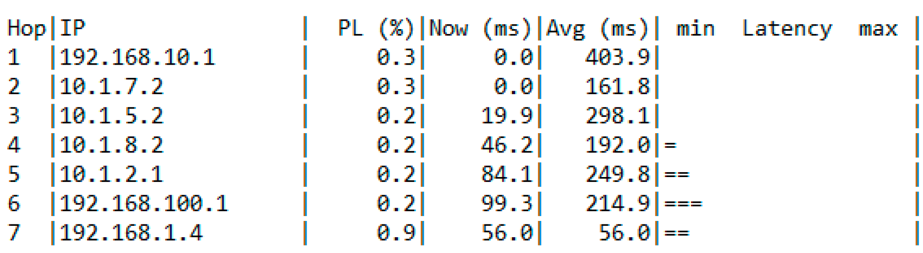
6.1.2. Results When Using OSPF and MPLS

Figure 13a shows the traffic generated at the output of the modeled network, i.e., the Router_Firewall interface. The sample interval was set at 1 s. As can be seen from the results, the traffic was again uneven (heterogeneous). The results were similar to those presented in Figure 2a. Figure 2b presents the results for the traffic generated across the entire measurement period. As can be seen, the traffic continued to be heterogeneous. The results were again similar to those of Figure 2b. From the obtained results, it can be seen that OSPF had no effect on the amount of traffic generated, which was expected and normal.
Figure 14 shows which protocols generated the most traffic. The HTTP generated the most traffic because of the 4K IP camera. The SSL protocol was used when accessing YouTube and other Internet pages.
Figure 15a,b show which TCP or UDP ports generated the most traffic. The results were again similar to the results presented in Figure 4a,b.
Figure 16a shows the distribution between broadcast and multicast packets. Again, the sample interval was set to 1 s for greater accuracy. The results were similar to those displayed in Figure 5a. Figure 16b presents the ratio between broadcast and multicast packets for the entire study period. Again, multicast packets dominated, as in Figure 5b.
Figure 17 shows the variation in the RTD between VM1 and the IP camera during the entire study. As can be seen, the obtained results were similar to those presented in Figure 6. Again, the large delay values were due to switching between the two operating modes of the IP camera and deleting and then restoring some of the links between the routers to check the operation of the OSPF protocol. The average value of the RTD over the entire study period was 291 ms; this was again a rather large delay value, which should not exceed, according to practice, 100 ms.
Figure 18 presents the results for the instantaneous RTD values between VM1 and the IP cam. The results were similar, like those presented in Figure 7. Again, the results were obtained under normal operation when no camera mode or network path changes were carried out (i.e., no router connections were deleted/restored).
Figure 19 shows the results captured when some of the links through which the packets passed in the above case had been deleted, and the packets were passing through a new, longer route. As can be seen from the results, the values were much higher than those in Figure 11. This showed that the use of OSPF led to a deterioration in the delay values. Such a dependence was also found by the authors of [41].
Figure 20 presents the mathematical distribution with beta approximation of packet size. As can be seen, the distribution was almost identical to that shown in Figure 9, with slight differences, such as a smaller number of packets, which was due to the shorter observation time compared to the previous study.
Figure 21a presents the mathematical distribution with Johnson SB approximation of the arrival times between the packets for the link between R1 and R6. The remaining links are not shown because they were continuously deleted/restored to verify the operation of the OSPF protocol. As can be seen, the time delay between packets was not constant. For a small slice of time, there was consistency in the arrival times. The obtained results when using OSPF were not as poor as when using EIGRP. Figure 21b presents the mathematical distribution with gamma approximation of the arrival times between packets for the link between R1 and Router_Firewall. Here, an uneven delay in packet arrival times was again noticeable. The obtained results were not as poor as those obtained for the network using EIGRP.

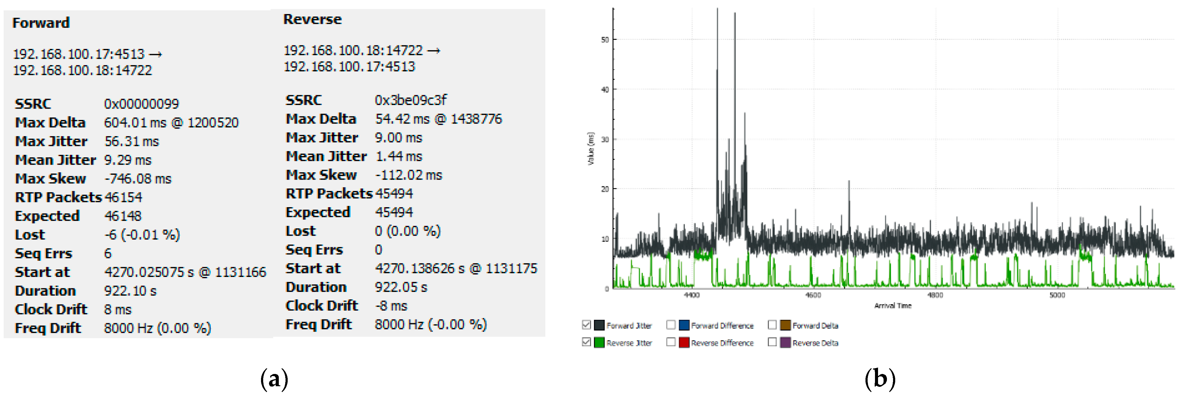
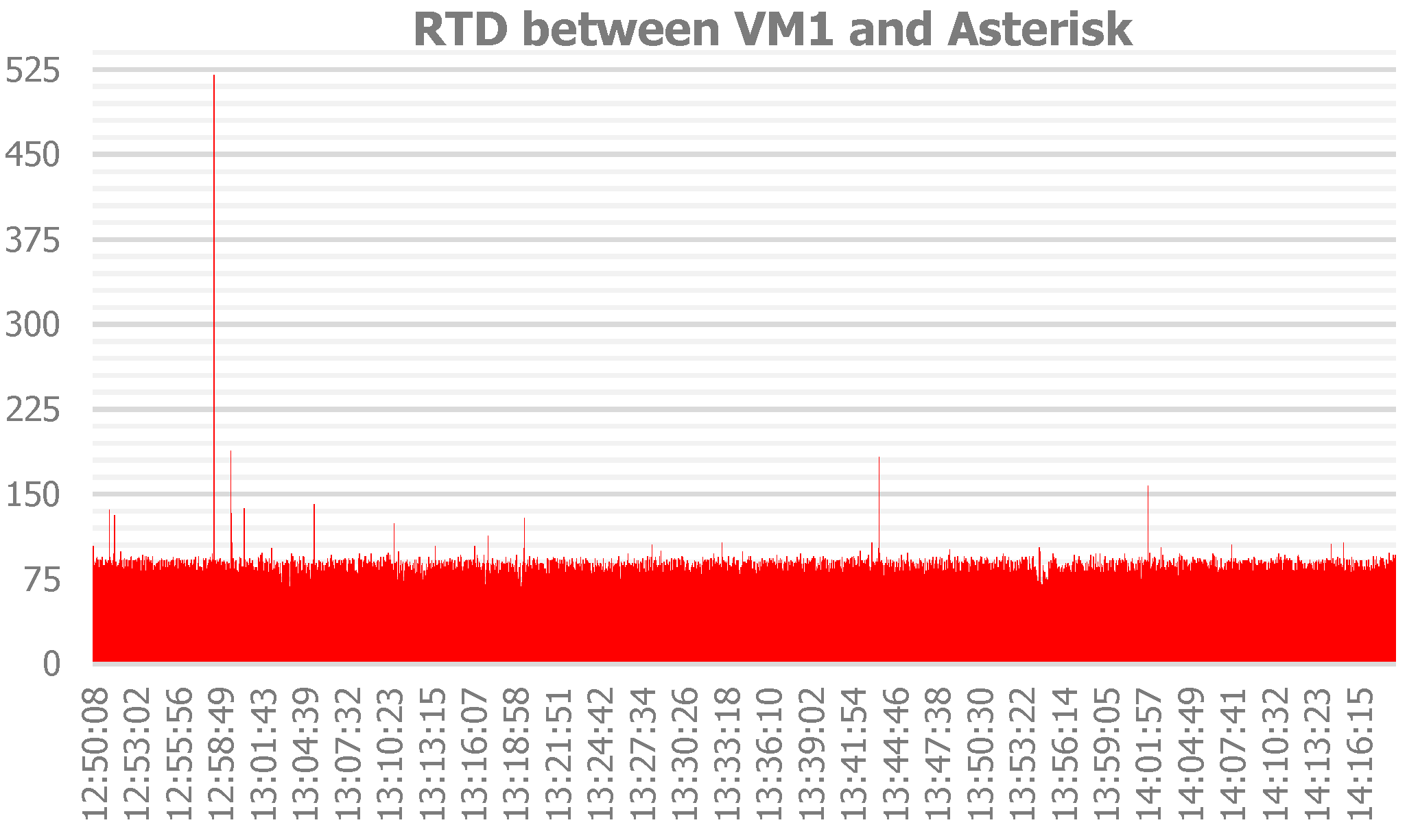
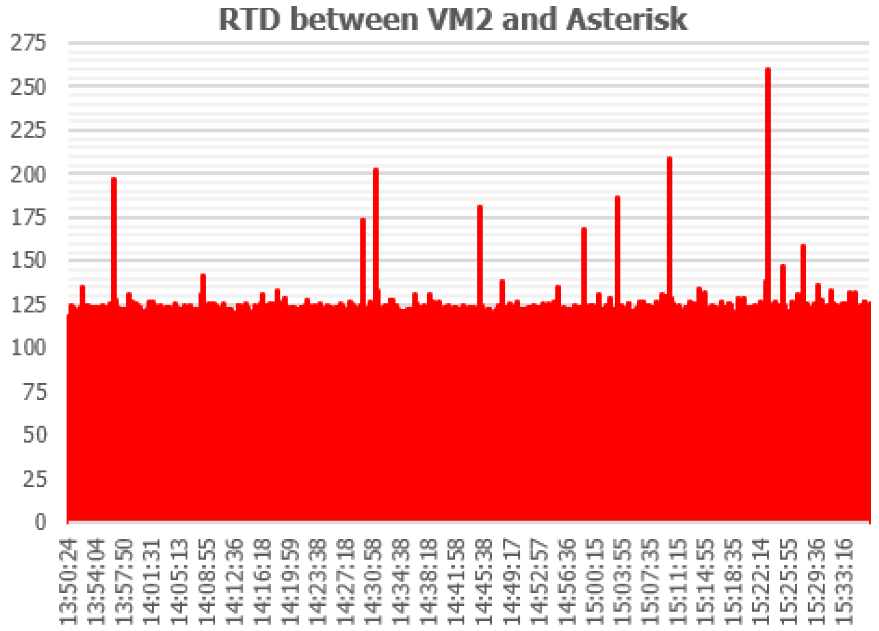
6.2. Model of a VoIP Network

Figure 22 shows the topology of the modeled VoIP network. It consisted of six routers (R1 to R6) and five switches (Switch 1 to Switch 5), to which four virtual machines (VM1 to VM4) were connected, representing the users/subscribers in the modeled VoIP network. Each of them made phone calls with every single virtual machine, as well as carrying out conference calls. For the IP phone PBX (Private Branch Exchange) the Asterisk Free PBX was chosen to be used. Asterisk Free PBX along with Router_Firewall were connected to the fifth switch (Switch 5). The modeled network exploited the ability of GNS3 to connect to real IP networks; in this case, the modeled network was connected to the Internet. Each of the virtual machines could access different resources on the Internet.
Again, the study was carried out in two parts. In the first part, the modeled IP network operated with the EIGRP and MPLS protocol. In the second part of the study, the modeled network operated with the OSPF and MPLS protocol. The purpose of the study was to verify under which of the two routing protocols the modeled network performed best when using MPLS technology, as well as to understand whether the routing protocols affected the performance of the modeled network implementing MPLS technology.

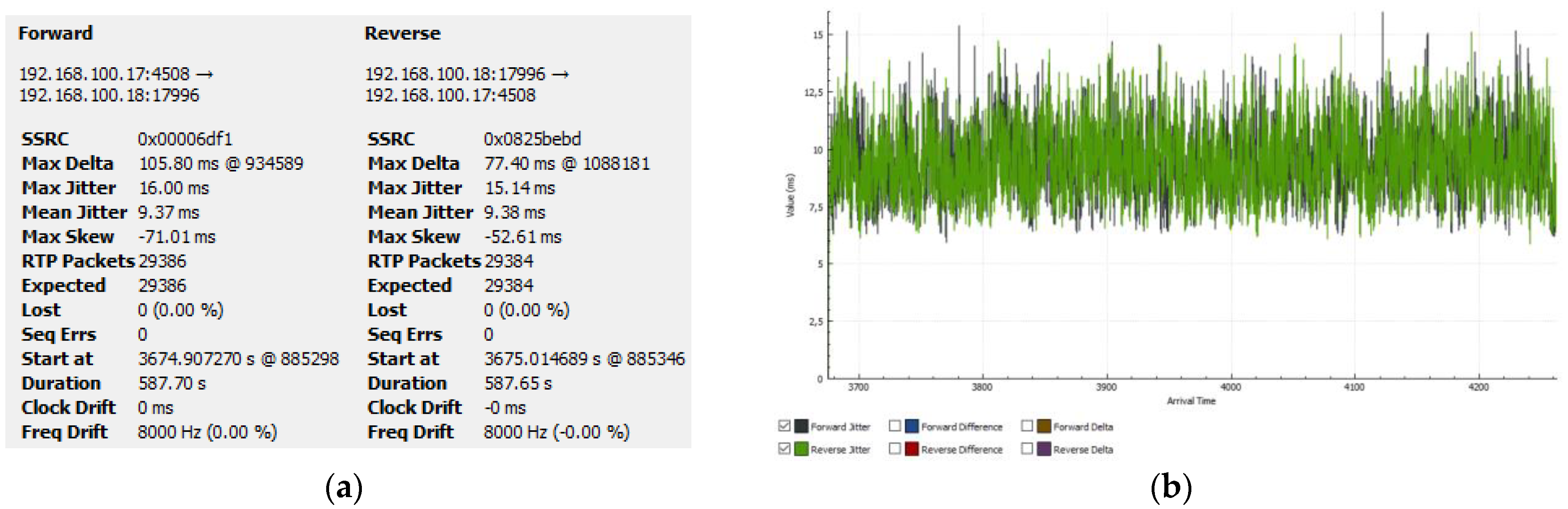
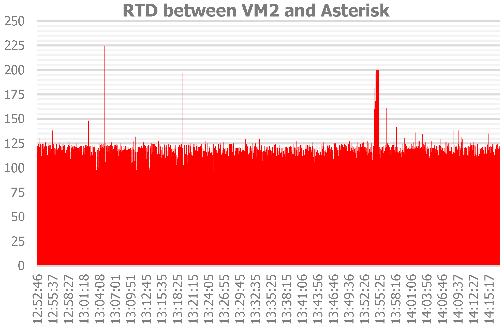
6.2.1. Results When Using EIGRP and MPLS

Figure 23a shows the traffic generated by the Asterisk Free PBX, which was measured over 1 s. As can be seen, the traffic was constant at around 100 KB/s, because it was only voice traffic. Figure 23b shows the traffic generated for the entire study period. Pauses in the traffic were due to moments of interruption/breakdown in already established telephone connections and the creation of new ones.
Figure 24 represents which protocol generated the most traffic. The HTTP generated the most traffic because the Asterisk Free PBX setup was implemented using a browser. In terms of the amount of traffic, compared to the second protocol (SIP—Session Initiation Protocol) the HTTP traffic is more, because the home page of the telephone exchange is animated, and this requires more data to be exchanged, compared to the SIP protocol, where the exchanged data is much smaller.
Figure 25a shows which TCP ports generated the most traffic. In this case, it was port 80, due to the accessing, monitoring, and configuring of the Asterisk Free PBX. As can be seen, there was no traffic over port 5060 (SIP). This was because the SIP in the Asterisk Free PBX was only exchanged over UDP. The remaining TCP ports were used for service information exchange. Figure 25b shows which UDP ports generated the most traffic. The Asterisk Free PBX worked with a large range of RTP ports (10,000–20,000), and everything outside this range was traffic exchanged with web pages with different content.
Figure 26 shows a summary of which ports (TCP or UDP) generated the most traffic. As can be seen from the obtained results, the traffic in the modeled network was mainly generated by UDP, which was normal for a multimedia-type network that exchanges traffic in real time.
Figure 27a shows the ratio between broadcast and multicast packets. The sample interval was set at 1 s for greater accuracy. As can be seen, only multicast packets were available, which was understandable, considering that in the modeled network the traffic was mainly multimedia-type real-time traffic. Figure 27b shows the ratio between broadcast and multicast packets for the entire period of the study. Again, it can be seen that the percentage of multicast packets was greater than that of broadcast packets. This indicated that the modeled network was functioning correctly.
The following section presents the results related to the performance of the modeled VoIP network.
Figure 28a presents the summarized results for a voice stream being exchanged between VM1 and the Asterisk Free PBX (VM1, R3, R2, R1, Asterisk, and vice versa). The results were obtained using a special function of Wireshark to examine the RTP (Real-Time Transport Protocol) streams. The main parameters that were monitored here were:
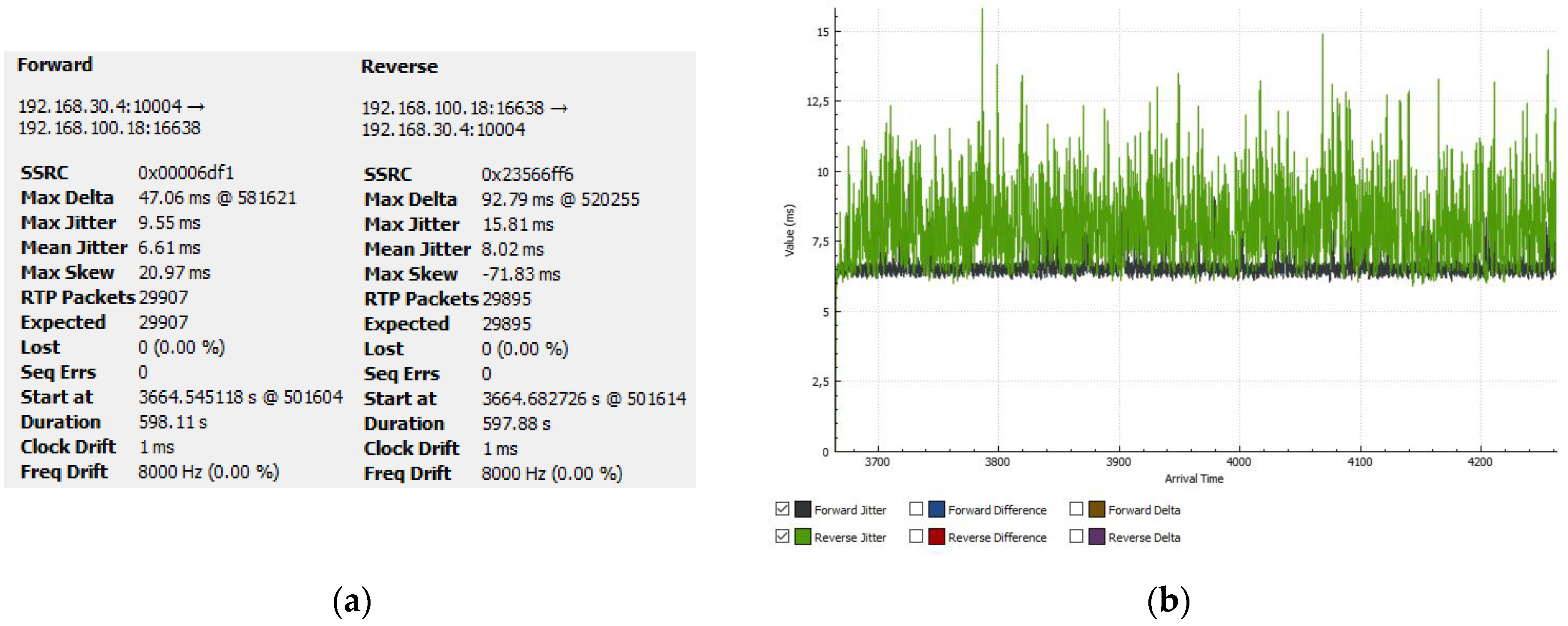
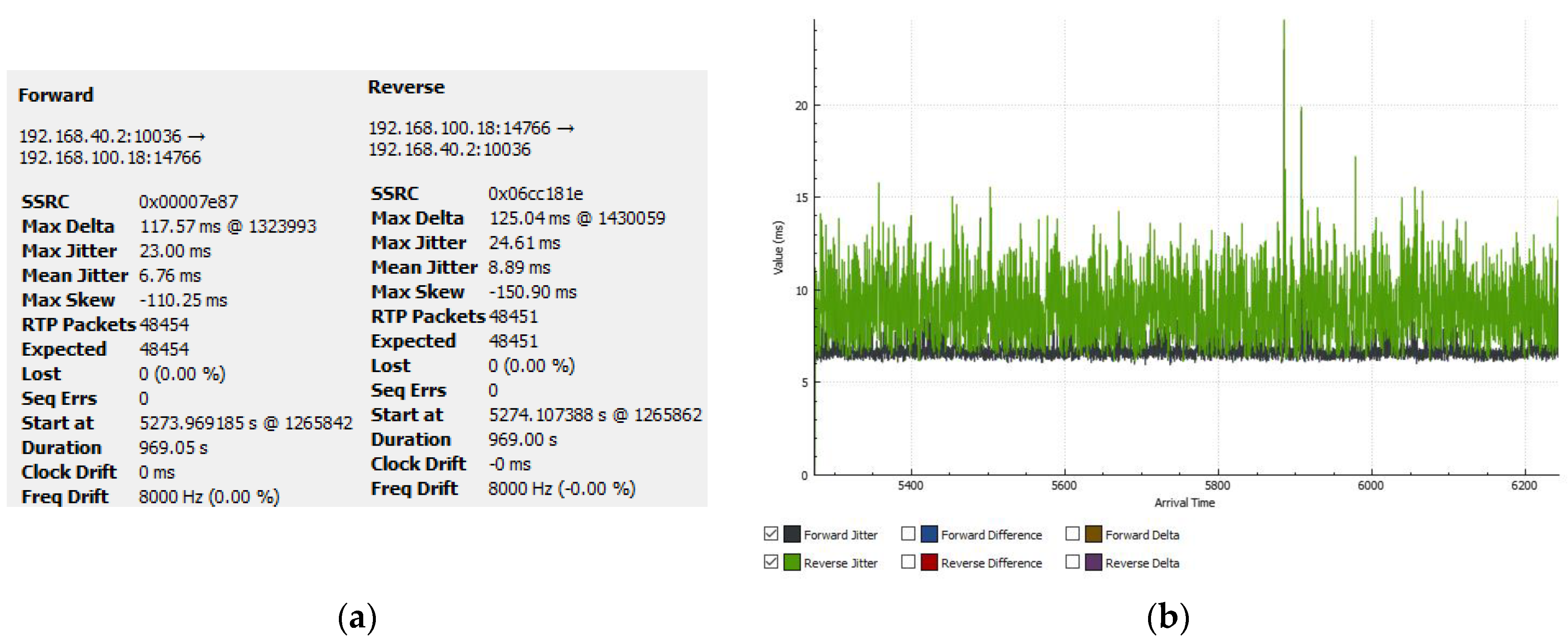
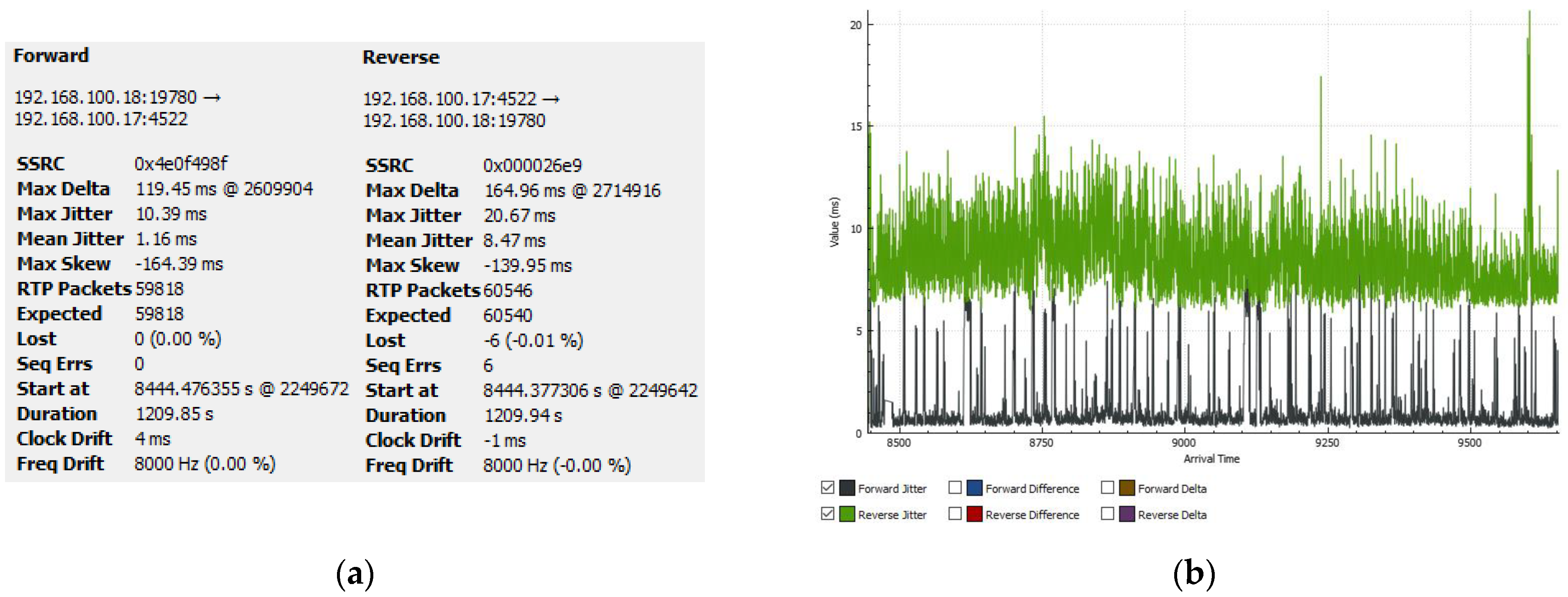
  • Packet loss: the results showed that there were no losses in the forward and reverse directions.
  • Information about the total number of RTP packets for each of the streams.
  • Information about the duration of the call—922 s.
  • Sampling frequency (8000 Hz; as can be seen, there was no deviation from this frequency for both directions), as well as the deviation from the clock frequency.
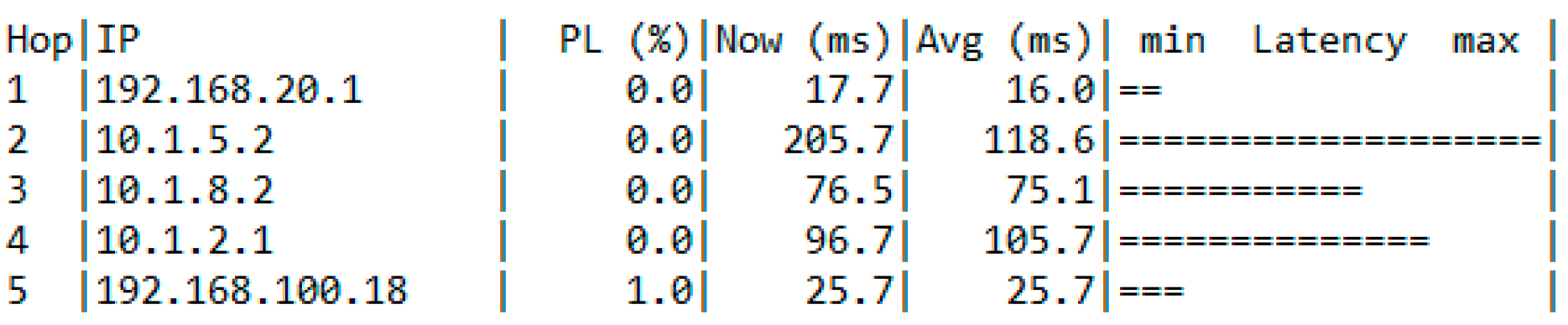
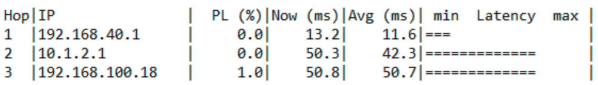
  • Information on the delay between the packets, following the delta and skew values: delta indicates the time difference between the receipt of the previous packet from the stream and the packet that has just been received. Skew indicates how long the current packet is ahead of or behind the entire call, relative to the nominal speed of the packet. In the presented case, it was noticed that the packet lagged behind the whole conversation.
  • Values of the max and mean jitter.
As can be seen from the results, the values of the jitter in both directions, from VM1 to the Asterisk and vice versa, were well below the limit of 30 ms [42,43]. The packet loss rate should be below 1% [42,43]. From the obtained results, it can be seen that in the modeled network, the values of these parameters were normal, and the model functioned normally. Figure 28b shows the variation in the jitter during the entire call for the voice stream studied in Figure 28a. As can be seen from the graph, the jitter only exceeded the instantaneous value of 30 ms a few times (three times), and only in the forward direction (VM1 to Asterisk). In the opposite direction, its values were below 20 ms.
Figure 29a shows the summarized results for the voice stream studied in Figure 28a, but examined at the Asterisk input/output. As can be seen, there was no particular change in the values of the parameters for the flow in the forward direction (VM1 to Asterisk). There was a slight increase in the average jitter value, which was normal; however, the packets from the voice stream passed through more routers before reaching the Asterisk. For the reverse flow (Asterisk to VM1), the values of the parameters were much better than those in Figure 28a, because this was where the reverse voice flow started. Figure 29b shows the variation in the jitter during the entire call for the voice stream studied in Figure 29a. For the voice stream in the forward direction (VM1 to Asterisk), the results were almost the same as those shown in the graph in Figure 28b. For the jitter values in the reverse direction (Asterisk to VM1), the results were much better than those presented in Figure 28b, because this was where the reverse voice stream started.
Figure 30 shows the variation in the RTD between VM1 and the Asterisk over the entire measurement period. As can be seen from the graph, the delay was almost constant and far from the allowable value of 300 ms for both directions (150 ms ineach direction) [42,43]. This graph further shows that the modeled network functioned normally.
Figure 31 presents the results for the instantaneous RTD values between VM1 and the Asterisk. The results were obtained using Solarwinds TracerouteNG; 192.168.10.1 was the gateway address of VM1, and 192.168.100.18 was the IP address of the Asterisk. As can be seen from the results, the delay across all the routers through which the packets passed was normal, well below 150 ms in this direction. These results confirmed the results of Figure 30.
Figure 32 presents the summarized results for a voice stream that was exchanged between VM2 and the Asterisk. The special characteristic of this flow was that it branched—the traffic in the forward direction (VM2 to Asterisk) passed through VM2, R4, R3, R2, R1, and the Asterisk; in the reverse direction, it passed through the Asterisk, R1, R6, R5, R4, and VM2. Therefore, there was also a difference in the results. As can be seen from Figure 32, the parameters of this voice stream were even better than those for the voice stream presented in Figure 29a.
Figure 33a shows the variation in the jitter over the entire call period for the VM2 to Asterisk direction. Figure 33b shows the jitter variation over the entire call period for the reverse direction (Asterisk to VM2). As can be seen from the two graphs, the jitter values were within the allowed limits, and the spikes that were observed in the voice stream between VM1 and the Asterisk were not noticeable.
Figure 34a shows the summarized results for the voice stream studied in Figure 32, but examined at the Asterisk input/output. As can be seen, there was no particular change in the values of the monitored parameters for the studied voice stream. The dependencies described for the voice stream between the Asterisk and VM1 also applied to this voice stream. Figure 34b shows the variation in the jitter during the entire call for the voice stream studied in Figure 34a. The obtained graphical results were better than those obtained for the Asterisk to VM1 voice stream presented in Figure 29b.
Figure 35 shows the variation in RTD between VM2 and the Asterisk over the entire measurement period. As can be seen from the graph, the delay was almost constant and substantially different from the allowable value of 300 ms for delay in both directions (150 ms in this direction). In contrast to the results of Figure 30, here the instantaneous values hovered around 120–130 ms.
Figure 36 presents the results for the instantaneous RTD values between VM2 and the Asterisk; 192.168.20.1 was the gateway address of VM2, and 192.168.100.18 was the IP address of the Asterisk. As can be seen from the results, the average value of the delay across all the routers through which the packets passed was normal, being below 150 ms in this direction. These results confirmed the results of Figure 35.
Figure 37a presents the summarized results for a voice stream that was exchanged between VM3 and the Asterisk (VM3, R5, R6, R1, Asterisk, and vice versa). The values of the parameters were again below the maximum allowable values and were much better than those obtained up to this point. Figure 37b shows the variation in the jitter during the entire call for the studied voice stream. The values were again within the norm.
Figure 38a shows the summarized results for the voice stream studied in Figure 37a, but examined at the Asterisk input/output. Figure 38b presents graphically the variation in the jitter for the entire duration of the call. As can be seen from both figures, there was no particular change in the values of the parameters for the two flows—the values were normal.
Figure 39 shows the variation in RTD between VM3 and the Asterisk over the entire measurement period. As can be seen from the graph, the delay was almost constant and substantially different from the allowable value of 300 ms for delay in both directions.
Figure 40 presents the results for the instantaneous RTD values between VM1 and the Asterisk; 192.168.30.1 was the gateway address of VM3, and 192.168.100.18 was the IP address of the Asterisk. As can be seen from the results, the average value of the delay across all routers through which the packets passed did not exceed the limit of 150 ms.
Figure 41a presents the summarized results for the voice stream that was exchanged between VM4 and the Asterisk (VM4, R6, R1, Asterisk, and vice versa). Again, the values of the monitored parameters were below the allowable limits. Figure 41b shows the variation in the jitter during the call for the studied voice stream. Again, the values were normal.
Figure 42a shows the summarized results for the voice stream studied in Figure 41a, but viewed at the Asterisk. Figure 42b presents the variation in the jitter across the entire call. As can be seen, there was no particular change in the values of the parameters for the two flows.
Figure 43 shows the variation in the RTD between VM4 and the Asterisk over the entire measurement period. The results were similar to those obtained so far. Figure 44 presents the results for the instantaneous RTD values between VM4 and the Asterisk; 192.168.40.1 was the gateway address of VM4, and 192.168.100.18 was the IP address of the Asterisk. As can be seen from the results, the values were normal.

6.2.2. Results When Using OSPF and MPLS

The results for the amount of generated traffic, the protocols and TCP/UDP ports that generated the most traffic, and the distribution between multicast and broadcast packets when using OSPF are not shown in this section, because they were almost the same as the results for the model using EIGRP and did not present any different or new information relevant to this study.
Figure 45a presents the summarized results for a voice stream that was exchanged between VM1 and the Asterisk (VM1, R3, R2, R1, Asterisk, and vice versa). As can be seen, there was a difference compared to the results for the voice stream when using EIGRP. An improvement was seen in the delta values as well as the maximum and average jitter values. Figure 45b shows the jitter variation over the entire call period. Except for a few peaks, the jitter value was within the allowed limits.
Figure 46a shows the summarized results for the voice stream studied in Figure 45a, but in the Asterisk to VM1 direction (at the Asterisk input/output interface). Again, there were slight improvements in the values compared to those of the voice traffic when using EIGRP. Figure 46b shows the jitter variation over the entire call period. Again, the values were within the norm, especially the values for the forward flow, which originated from the Asterisk.
Figure 47 shows the variation in the RTD between VM1 and the Asterisk over the entire measurement period. The results showed that the delay was constant, presenting almost the same values as the studied voice flow between VM1 and the Asterisk when using EIGRP.
Figure 48 presents the results for the instantaneous RTD values between VM1 and the Asterisk. As can be seen, the results were almost identical to those obtained when using EIGRP.
Figure 49 shows the summarized results for a voice stream that was exchanged between VM2 and the Asterisk (VM2, R4, R5, R6, R1, Asterisk). The reverse voice flow again followed another path, just as when using EIGRP (Asterisk, R1, R2, R3, R4, VM2). Here, the parameter values were higher than those for the studied voice flow when using EIGRP.
Figure 50a,b show the jitter variation over the entire call period. Regardless of the path taken by the voice packets, the values were still normal.
Figure 51a shows the summarized results for the voice stream exchanged between the Asterisk and VM2, originating from the Asterisk. The values of the parameters in the reverse direction were higher than the values for the voice flow observed when using EIGRP. Figure 51b shows the jitter variation over the entire call period for the voice stream presented in Figure 49. The results were similar to those of Figure 50a,b.
Figure 52 presents the results for the instantaneous RTD values between VM2 and the Asterisk. As can be seen, the results were identical to those obtained when using the EIGRP. The Solarwinds TracerouteNG results for the RTD (Figure 53) were slightly worse than when using EIGRP.
Figure 54a presents the summarized results for a voice stream between VM3 and the Asterisk (VM3, R5, R6, R1, Asterisk, and vice versa). In terms of the average jitter, the results were close to those of the examined voice stream using the EIGRP. The delta values were higher, but these were momentary peaks. Figure 54b shows the jitter variation over the entire call period for the voice stream presented in Figure 54a. The results were again identical to those for the voice stream studied using EIGRP.
Figure 55a presents the summarized results for the voice stream examined in Figure 54a, but starting from the Asterisk. Figure 55b shows the jitter variation over the entire call period for the voice stream of Figure 55a. The results were close to those obtained in the voice stream study when using EIGRP for the same path from the Asterisk to VM3.
Figure 56 presents the variation in RTD between VM3 and the Asterisk over the entire study period. The results were again similar to those obtained using EIGRP. The results for the instantaneous round-trip delay values between VM3 and the Asterisk (Figure 57) were also close to those obtained using EIGRP.
Figure 58a presents the summarized results for a voice stream that was exchanged between VM4 and the Asterisk (VM4, R6, R1, Asterisk, and vice versa). No major deviations in the values were noticed, and everything was again within the norm. Figure 58b plots the variation in the jitter in both directions over the entire duration of the call for the voice stream studied in Figure 58a. Again, the values were within the normal range.
Figure 59a shows the summarized data for the studied voice stream of Figure 58a, but starting from the Asterisk. Again, the values of the monitored parameters were normal. Figure 59b graphically represents the jitter variation over the entire call period for the voice stream of Figure 59a. Again, the jitter variation was within acceptable limits.
Figure 60 shows the instantaneous values of the RTD. The values were again normal, but slightly better than the values obtained in the study using EIGRP.
Figure 61 graphically presents the variation in the RTD for the entire studied period. The results were identical to those for the study using EIGRP.

6.3. Using the IP Network Modeling Platforms to Study Power Electronic Devices

The platforms for modeling IP networks can also be used in the study of power electronic devices (PEDs) [44,45] to characterize the communication traffic that they generate. Why use IP network modeling platforms in PED research? The need mainly arises from the impossibility of creating experimental, physical networks due to the lack of network devices such as switches and/or routers. Their absence may be due to, for example, a lack of financial opportunities to purchase such network equipment. Using IP network modeling platforms solves this problem. In the present work, GNS3 was applied to characterize the communication traffic generated by PEDs.
Such studies are necessary to facilitate the design/choice of the most suitable communication network to which the studied PED can be connected—whether it be an existing IP network or the data network of a mobile operator, or whether studying if connecting a PED affects the performance of an already established IP network. All this can only be found out if a thorough characterization of the communication traffic generated by the PED is carried out.
Figure 62 presents the topology of the modeled IP network that was used to characterize the communication traffic. The studied PED was a Power Distribution Unit (PDU). This power device is used by telecommunications operators to remotely control the power supply of various telecommunications devices and modules (switches, routers, etc.). To characterize the generated communication traffic, the tools mentioned above were used again: Capsa 11 free, Wireshark, and mathematical distributions by packet size. The distributions of arrival times between packets were not used, because when characterizing the communication traffic from one PED, it was the only device in the experimental network; thus, the information from such a distribution was redundant and did not provide any significant data that would be useful for this study.
Figure 63a presents the generated traffic from the studied PDU for a sample interval of 1 s (to achieve maximum accuracy). The graph shows that the generated traffic was minimal and at times non-existent. When the device was not accessible, no traffic was generated. Figure 63b presents the traffic generated by the studied PDU for the entire study period. For the studied period, it can be seen that there was not much traffic, and there was even a period where no traffic was generated.
Figure 64 presents the results for the protocols generating the most traffic in the network. The HTTP generated the most traffic, because the examined PDU was only accessible through a browser.
Figure 65 presents information on the ports (TCP or UDP) from which the most traffic was generated. From the graph, it can be seen that the most traffic was generated from TCP port 80, which was normal; however, the studied PDU was only accessible through a browser. The remaining TCP ports were used to maintain the session between the PDU and the VM1 workstation.
When characterizing the communication traffic from the PED, it was desirable to verify whether the data exchange between the PED and the control station (VM1) was secure. This could be accomplished using Wireshark. Figure 66 demonstrates the results of this check. As can be seen, the device access information, such as username “admin” and password “password”, was exchanged in plane text.
Figure 67 presents the mathematical distribution by packet size with Cauchy approximation. From the distribution, it is clear that the packets with sizes of 100 bytes and 600 bytes were the most common. These were basic service packets to maintain the session between the workstation and the PDU. Packets with sizes of 1500 bytes and 1200 bytes were used to transmit statistical data and the graphical layout of the Internet page through which the PDU management took place.
Through the IP network modeling platforms, various methods and techniques can be tested to improve the performance of the modeled network. For the studied topology shown in Figure 62, various techniques could be applied to improve and ensure secure data exchange between the studied PDU and the monitoring and control station (VM1). Figure 68 presents the topology of a modeled network through which VPN technology was used to implement secure data exchange. The tunnel was created between R1 and R5. The IPSec protocol was used. Additionally, the modeled network was provided with access to the Internet using pfSense and the ability of GNS3 to connect modeled IP networks to real IP networks. VM1 exchanged traffic, both with the studied PDU and to access various resources on the Internet.
Figure 69 shows the Wireshark results verifying that the tunnel was functional while also exchanging traffic with other devices somewhere in the world. The data exchange between the VM1 and the PDU was secure. Other methods for secure data exchange are discussed in [46,47].
Finally, with the help of IP network modeling platforms, different hypotheses can be verified. The research presented herein tested the hypothesis “will there be any changes in the performance of an IP network when a PED is connected to a working IP network?”. For this purpose, the studied PDU was added to the topology of Figure 1.
Figure 70 presents the generated traffic for the entire study period. Compared to the results shown in Figure 2b, when the PDU was not connected to the network, the traffic was still heterogeneous. No significant differences were noticeable.
Figure 71 shows which protocols generated the most traffic. The difference in Figure 3 arose from the fact that in this study, the IP camera was not accessed as often; instead, different resources on the Internet, such as different YouTube channels, were mainly accessed.
Figure 72 presents the mathematical distribution with beta approximation of packet size. The distribution appeared almost the same as the results presented in Figure 9, with slight differences, such as an increase in packets up to 100 bytes in size, as well as packets up to 1300 bytes in size. This was due to the addition of the investigated PDU.

7. Discussion

7.1. Results and Discussion for Section 6.1

In Section 6.1, a working model of an IP network was created that was connected to a real network (the Internet) and exchanged traffic with various devices on the Internet. Dynamic protocols performed their tasks and were constantly ready to activate the backup routes from the routing tables when necessary—for example, when some of the existing links between the routers failed. This was carried out and can be seen in the results for the instantaneous RTD values, with the packets passing through one path for some results and another path for other results. The purpose of the developed IP network model was to verify whether the use of different dynamic routing protocols had any impact on the performance of MPLS technology.
The traffic characterization performed for the two operating modes of the modeled network (using EIGRP or OSPF) showed identical results. In both versions of the network, the traffic was heterogeneous, which was normal for multimedia-type networks (both versions of the model were multimedia-type networks). This was also confirmed by the results for the distribution between broadcast and multicast packets—multicast packets were much more common and dominated compared to broadcast packets. The results of the mathematical distributions for packet size for both networks were identical.
Regarding the time delay in the two versions of the investigated topology, no significant differences were noticeable. In the network using EIGRP, slightly better instantaneous values of time delay were observed. This could be seen in the Solarwinds TracerouteNG results. Due to these smaller values, the difference in the mathematical distributions of the packet arrival times was also obtained, and improvements were noticeable compared to the same results obtained for the network using OSPF. It is important to note that in both versions of the studied network, the settings of the dynamic routing protocols were based on the default. No QoS (Quality of Service) was set. Therefore, using EIGRP always showed slight improvements over using OSPF for the same network.
In summary, the following can be stated: based on the results obtained by studying the two versions of the modeled network, no significant differences in the performance of the network were noticed when using MPLS with EIGRP or OSPF.

7.2. Results and Discussion for Section 6.2

In Section 6.2, a working model of a VoIP network was created in which voice streams were exchanged (telephone calls were made between subscribers). Additionally, the modeled VoIP network was connected to a real network (the Internet), and virtual workstations could access various resources (open Internet pages). In both versions of the studied network, the settings of the dynamic routing protocols were based on the default. No QoS was set. The purpose of the developed IP network model was to verify whether the use of different dynamic routing protocols had any impact on the performance of MPLS technology when using the technology in a VoIP network.
During the traffic characterization, for both versions of the studied model network, it was confirmed that the model functioned correctly as a network in which multimedia traffic was exchanged. The generated traffic was homogeneous and constant, which was typical of a VoIP network where mainly voice traffic was exchanged, as was the case for the studied model network. When using EIGRP and OSPF, there was almost no difference in the results for generated traffic, generated traffic per port, and other parameters.
In the performance study, again, there was not much difference in the performance of the modeled network when using EIGRP or OSPF. With both protocols, the time delay in all studied links was constant and presented almost the same values. The average and maximum jitter values were almost the same and within acceptable limits (below 30 ms) for the average jitter value. The instantaneous RTD values were also within the permissible values (below 150 ms in one direction).
In summary, it can be argued that when using EIGRP and OSPF, there was almost no difference in network performance when applying MPLS technology.

7.3. Results and Discussion for the Results from Section 6.3

Section 6.3 discussed the capabilities of the IP network modeling platforms for PED research. The characterization of the communication traffic generated by the PED study proved the hypothesis that PEDs do not generate much traffic. This was confirmed by the obtained results, and it could even be seen that there were times when no traffic was generated at all. From the mathematical distribution, it could be seen that for the PED study, the largest percentage of all packets were those with sizes of 100 bytes and 600 bytes. The security of the exchanged information was seen to be lacking. Important information such as usernames, passwords, and control commands were transmitted in plain text. This was unacceptable, because in today’s world, any device connected to the Internet can be the subject of an attack. Transmitted in this way, important information can very easily be intercepted. As a result, the device could be compromised and misused—instead of the communication or other equipment powered by the PDU being controlled by the right people, it can be remotely controlled by other people; thus, the equipment is compromised and cannot be used as intended. Solutions to this problem are achieved via the use of various technologies and methods for secure data exchange. This article proposed the use of VPN technology. A tunnel was created in the modeled network through which information was exchanged between the PDU and VM1 (control center). Thus, no one could “connect” and manipulate the information exchanged.
Regarding the hypothesis that connecting a PED to an already operational IP network would result in changes in the performance of the IP network, such concerns proved to be unnecessary. The connection of the PED to an already built and functioning IP network did not lead to any changes in its performance. This was proven by the presented results.
In summary, it can be argued that the use of IP network modeling platforms is very suitable for the study of PEDs.

8. Conclusions

Working models of IP networks used for various purposes were created.
The use of GNS3 for the modeling of IP networks was proposed. Its main advantages were presented. A set of tools for monitoring and analyzing the processes in the modeled IP networks was proposed.
From the obtained results, it could be seen that the use of EIGRP or OSPF did not lead to any changes in the functioning of the MPLS technology. This was true for both studied IP network models.
IP network modeling platforms are suitable and convenient for characterizing communication traffic from power electronic devices.
Thanks to the use of platforms for modeling IP networks, one of the main problems for every educational institution can be solved—the lack of financial means for the purchase of expensive network equipment. By using these platforms, IP networks can be created from network devices running operating systems on real network devices. Thus, the models are as close as possible to real such networks.
With IP network modeling platforms, IP networks can be created with different numbers of network devices. Creating a physical experimental network composed of several to tens of network devices is difficult to implement. There are no such restrictions in IP network modeling platforms. Limitations on the number of the modeled devices are due to the computing capabilities of the workstation that is used to model IP networks.
Various scenarios can be created through these platforms that are necessary for the study of a given IP network or communication technology.
Last but not least, the platforms are convenient for conducting distance learning.
Of course, the proposed platforms also have disadvantages. The main disadvantage is the need for powerful computing capabilities for the workstations that will be used to model the IP networks. This means that it is necessary to invest some money in assembling a powerful enough workstation that can be used to model the IP networks. These financial costs will be much lower than the financial costs required to purchase the network equipment.

Funding

This research received no external funding.

Institutional Review Board Statement

Not applicable.

Informed Consent Statement

Not applicable.

Data Availability Statement

Not applicable.

Conflicts of Interest

The author declares no conflict of interest.

References

  1. CV, R.K.; Goyal, H. IPv4 to IPv6 Migration and Performance Analysis Using GNS3 and Wireshark. In Proceedings of the 2019 International Conference on Vision towards Emerging Trends in Communication and Networking (ViTECoN), Vellore, India, 30–31 March 2019; pp. 1–6. [Google Scholar] [CrossRef]
  2. Kurniawan, D.E.; Kushardianto, N.C.; Thohari, A.H. Simulation and Analysis Network Performance of IPv4, IPv6 and ISATAP Tunneling on Polibatam Network Laboratory. In Proceedings of the 2019 2nd International Conference on Applied Engineering (ICAE), Batam, Indonesia, 2–3 October 2019; pp. 1–4. [Google Scholar] [CrossRef]
  3. Qaid, A.; Ertuğ, Ö. Transition from IPv4 to IPv6 Mechanisms by GNS3 Emulation: YPTC as a Case Study. In Proceedings of the 2021 International Symposium on Networks, Computers and Communications (ISNCC), Dubai, United Arab Emirates, 31 October–2 November 2021; pp. 1–7. [Google Scholar] [CrossRef]
  4. Fahmi; Muladi; Ashar, M.; Wibawa, A.P.; Purnawansyah. IPv6 vs IPv4 Performance Simulation and Analysis Using Dynamic Routing OSPF. In Proceedings of the 2021 4th International Conference of Computer and Informatics Engineering (IC2IE), Depok, Indonesia, 14–15 September 2021; pp. 452–456. [Google Scholar] [CrossRef]
  5. Ogudo, K.A. Analyzing Generic Routing Encapsulation (GRE) and IP Security (IPSec) Tunneling Protocols for Secured Communication over Public Networks. In Proceedings of the 2019 International Conference on Advances in Big Data, Computing and Data Communication Systems (icABCD), Winterton, South Africa, 5–6 August 2019; pp. 1–9. [Google Scholar] [CrossRef]
  6. Biradar, A.G. A Comparative Study on Routing Protocols: RIP, OSPF and EIGRP and Their Analysis Using GNS-3. In Proceedings of the 2020 5th IEEE International Conference on Recent Advances and Innovations in Engineering (ICRAIE), Jaipur, India, 1–3 December 2020; pp. 1–5. [Google Scholar] [CrossRef]
  7. Mounika, P. Performance analysis of wireless sensor network topologies for Zigbee using riverbed modeler. In Proceedings of the 2018 2nd International Conference on Inventive Systems and Control (ICISC), Coimbatore, India, 19–20 January 2018; pp. 1456–1459. [Google Scholar] [CrossRef]
  8. Jain, N.; Payal, A. Comparison between IPv4 and IPv6 Using OSPF and OSPFv3 on Riverbed Modeler. In Proceedings of the 2019 IEEE International Conference on Advanced Networks and Telecommunications Systems (ANTS), Goa, India, 16–19 December 2019; pp. 1–7. [Google Scholar] [CrossRef]
  9. Parwani, R.; Al-Amoudi, H.M.S.; Jhummarwala, A. Modeling and Simulating large scale Cyber Effects for Cybersecurity Using Riverbed Modeler. In Proceedings of the 2020 10th International Conference on Cloud Computing, Data Science & Engineering (Confluence), Noida, India, 29–31 January 2020; pp. 570–575. [Google Scholar] [CrossRef]
  10. Yihunie, F.; Abdelfattah, E.; Odeh, A. Analysis of ping of death DoS and DDoS attacks. In Proceedings of the 2018 IEEE Long Island Systems, Applications and Technology Conference (LISAT), Farmingdale, NY, USA, 4 May 2018; pp. 1–4. [Google Scholar] [CrossRef]
  11. Mittal, R.; kazim, A. Ananlysis of DDoS Attacks In Cloud. In Proceedings of the 2020 International Conference on Smart Technologies in Computing, Electrical and Electronics (ICSTCEE), Bengaluru, India, 9–10 October 2020; pp. 19–23. [Google Scholar] [CrossRef]
  12. Konshin, S.; Yakubova, M.Z.; Nishanbayev, T.N.; Manankova, O.A. Research and Development of an IP network model based on PBX Asterisk on the Opnet Modeler simulation package. In Proceedings of the 2020 International Conference on Information Science and Communications Technologies (ICISCT), Karachi, Pakistan, 8–9 February 2020; pp. 1–5. [Google Scholar] [CrossRef]
  13. Salian, R. Performance Analysis of Voice over WLAN Intercom System and Optimized Implementation for Android Users. In Proceedings of the 2020 11th International Conference on Computing, Communication and Networking Technologies (ICCCNT), Kharagpur, India, 1–3 July 2020; pp. 1–7. [Google Scholar] [CrossRef]
  14. Ishgeem, O.A.; Abood, A.M.; Abosata, N.R.; Alzawam, H.A.; Haqaf, H.T. Analysis and Evaluation QoS of VoIP over WiMAX and UMTS Networks. In Proceedings of the 2021 IEEE 1st International Maghreb Meeting of the Conference on Sciences and Techniques of Automatic Control and Computer Engineering MI-STA, Tripoli, Libya, 25–27 May 2021; pp. 787–793. [Google Scholar] [CrossRef]
  15. Jarjis, A.; Kadir, G. Blockchain Authentication for AODV Routing Protocol. In Proceedings of the 2020 Second International Conference on Blockchain Computing and Applications (BCCA), Antalya, Turkey, 2–5 November 2020; pp. 78–85. [Google Scholar] [CrossRef]
  16. Jiang, C.; Yang, Y.; Chen, X.; Liao, J.; Song, W.; Zhang, X. A New-Dynamic Adaptive Data Rate Algorithm of LoRaWAN in Harsh Environment. IEEE Internet Things J. 2022, 9, 8989–9001. [Google Scholar] [CrossRef]
  17. Wang, Y.; Peng, L.; Xu, R.; Yang, Y.; Ge, L. A Fast Neighbor Discovery Algorithm Based on Q-learning in Wireless Ad Hoc Networks with Directional Antennas. In Proceedings of the 2020 IEEE 6th International Conference on Computer and Communications (ICCC), Chengdu, China, 11–14 December 2020; pp. 467–472. [Google Scholar] [CrossRef]
  18. Li, F.; Gao, W.; Chen, L.; Liu, W. Modeling and Simulation of Network-on-Chip Routing Algorithm Based on OPNET. In Proceedings of the 2020 International Conference on Intelligent Computing and Human-Computer Interaction (ICHCI), Sanya, China, 4–6 December 2020; pp. 323–327. [Google Scholar] [CrossRef]
  19. Jha, C.K.; Yosef Zorkta, H.; Al-Saleh, A.H.; Nor-Al-Deen Fakhrow, F. New Queuing Technique for Improving Computer Networks QoS. In Proceedings of the 2020 International Conference for Emerging Technology (INCET), Belgaum, India, 5–7 June 2020; pp. 1–5. [Google Scholar] [CrossRef]
  20. Panhwar, M.A.; Memon, K.A.; Abro, A.; Zhongliang, D.; Khuhro, S.A.; Ali, Z. Efficient Approach for optimization in Traffic Engineering for Multiprotocol Label Switching. In Proceedings of the 2019 IEEE 9th International Conference on Electronics Information and Emergency Communication (ICEIEC), Beijing, China, 12–14 July 2019; pp. 1–7. [Google Scholar] [CrossRef]
  21. Tasho, D.T.; Marin, B.M.; Radostina, P.T.; Alexander, K.A. Generalized nets model of the LPF-algorithm of the crossbar switch node for determining LPF-execution time complexity. In Proceedings of the AIP Conference 2333, 090039 (2021), Sofia, Bulgaria, 7–13 June 2020. [Google Scholar] [CrossRef]
  22. Peng, J.; Michael, G.; Kimmig, A.; Marinov, M.B.; Wang, J.; Ovtcharova, J. An Advanced IoT Platform and its Implementations Focused on Modern Information Technology Generation. In Proceedings of the 2020 XI National Conference with International Participation (ELECTRONICA), Sofia, Bulgaria, 23–24 July 2020; pp. 1–4. [Google Scholar] [CrossRef]
  23. Mirtchev, S.T. Investigation of Pareto/M/1/k Teletraffic System by Simulation. In Proceedings of the 2019 27th National Conference with International Participation (TELECOM), Sofia, Bulgaria, 30–31 October 2019; pp. 70–73. [Google Scholar]
  24. Getting Started with GNS3. Available online: https://docs.gns3.com/docs/ (accessed on 7 January 2023).
  25. Colasoft Ping Tool. Available online: https://www.colasoft.com/ping_tool/ (accessed on 7 January 2023).
  26. Soalrwinds Traceroute NG. Available online: https://www.solarwinds.com/free-tools/traceroute-ng (accessed on 7 January 2023).
  27. Capsa Free Network Analyzer. Available online: https://www.colasoft.com/capsa-free/ (accessed on 7 January 2023).
  28. Wireshark. Available online: https://www.wireshark.org/docs/wsug_html_chunked/ (accessed on 7 January 2023).
  29. Mohammed, M.A. Mathematical Approximation of Delay in Voice over IP. Int. J. Comput. Inf. Technol. 2014, 3, 78–82. [Google Scholar]
  30. Hammad, K.; Moubayed, A.; Shami, A.; Primak, S. Analytical Approximation of Packet Delay Jitter in Simple Queues. IEEE Wirel. Commun. Lett. 2016, 5, 564–567. [Google Scholar] [CrossRef]
  31. Marinov, M.B.; Nikolov, N.; Dimitrov, S.; Todorov, T.; Stoyanova, Y.; Nikolov, G.T. Linear Interval Approximation for Smart Sensors and IoT Devices. Sensors 2022, 22, 949. [Google Scholar] [CrossRef] [PubMed]
  32. The pfSense Documentation. Available online: https://docs.netgate.com/pfsense/en/latest/preface/index.html (accessed on 7 January 2023).
  33. Mirtchev, S.T. Packet-Level Link Capacity Evaluation for IP Networks. Cybern. Inf. Technol. 2018, 18, 30–40. [Google Scholar] [CrossRef] [Green Version]
  34. Sapundzhi, F.I.; Popstoilov, M.S. Optimization Algorithms for Finding the Shortest Paths. Bulg. Chem. Commun. 2018, 50, 115–120. [Google Scholar]
  35. Sapundzhi, F.; Popstoilov, M. C # implementation of the maximum flow problem. In Proceedings of the 2019 27th National Conference with International Participation (TELECOM), Sofia, Bulgaria, 30–31 October 2019; pp. 62–65. [Google Scholar]
  36. Cherneva, G.P.; Hristova, V.I. Evaluation of FHSSS Stability against Intentional Disturbances. In Proceedings of the 2020 28th National Conference with International Participation (TELECOM), Sofia, Bulgaria, 29–30 October 2020; pp. 14–16. [Google Scholar] [CrossRef]
  37. Cherneva, G.P. Control of the Chaotic Processes in Chaos Shift Keying Communication System. In Proceedings of the 2019 27th National Conference with International Participation (TELECOM), Sofia, Bulgaria, 30–31 October 2019; pp. 1–3. [Google Scholar] [CrossRef]
  38. Siswanto, A.; Syukur, A.; Kadir, E.A.; Suratin. Network Traffic Monitoring and Analysis Using Packet Sniffer. In Proceedings of the International Conference on Advanced Communication Technologies and Networking (CommNet), Rabat, Morocco, 12–15 April 2019; pp. 1–4. [Google Scholar] [CrossRef]
  39. Sinchana, K.; Sinchana, C.; Gururaj, H.L.; Sunil Kumar, B.R. Performance Evaluation and Analysis of various Network Security tools. In Proceedings of the International Conference on Communication and Electronics Systems (ICCES), Coimbatore, India, 17–19 July 2019; pp. 644–650. [Google Scholar]
  40. Sapundzhi, F.I.; Popstoilov, M.S. Maximum-Flow Problem in Networking. Bulg. Chem. Commun. 2020, 52, 192–196. [Google Scholar]
  41. Teshabayev, T.; Yakubova, M.; Nishanbaev, T.; Yakubov, B.; Golubeva, T.; Sadikova, G. Analysis and research of capacity, latency and other characteristics of backbone multiservice networks based on simulation modeling using different routing protocols and routers from various manufacturers for using the results when designing and modernization of multiservice networks. In Proceedings of the International Conference on Information Science and Communications Technologies, Tashkent, Uzbekistan, 4–6 November 2019; pp. 1–7. [Google Scholar]
  42. Tim, S.; Christina, H. End-to-End QoS Network Design: Quality of Service in LANs, WANs, and VPNs. In Part of the Networking Technology Series; Cisco Press: Indianapolis, Indiana, 2004; ISBN -10: 1-58705-176-1. [Google Scholar]
  43. Cisco-Understanding Delay in Packet Voice Networks, White Paper. Available online: https://www.cisco.com/c/en/us/support/docs/voice/voice-quality/5125-delay-details.html (accessed on 7 January 2023).
  44. Kishkin, K.K.; Stefanov, I.T.; Arnaudov, D.D. Virtual Instrument for Capacitance Measurement of Supercapacitor Cells as part of an Energy Storage System. In Proceedings of the XXXI International Scientific Conference Electronics (ET), Sozopol, Bulgaria, 13–15 September 2022; pp. 1–5. [Google Scholar] [CrossRef]
  45. Kishkin, K.; Kanchev, H.; Arnaudov, D. Modeling the Influences of Cells Characteristics in Battery Bank. In Proceedings of the 22nd International Symposium on Electrical Apparatus and Technologies (SIELA), Bourgas, Bulgaria, 1–4 June 2022; pp. 1–5. [Google Scholar] [CrossRef]
  46. Dimitrov, W. The Impact of the Advanced Technologies over the Cyber Attacks Surface. In Artificial Intelligence and Bioinspired Computational Methods. CSOC 2020; Silhavy, R., Ed.; Advances in Intelligent Systems and Computing; Springer: Cham, Switzerland, 2020; Volume 1225. [Google Scholar] [CrossRef]
  47. Willian, A.D.; Galina, S.P. The Impacts of DNS Protocol Security Weaknesses. J. Commun. 2020, 15, 722–728. [Google Scholar] [CrossRef]
Figure 1. Topology of the modeled IP network.
Computers 12 00041 g001
Figure 2. (a) Total generated traffic when the sample interval was set to 1 s when using EIGRP; (b) total generated traffic for the whole period of the study when using EIGRP.
Computers 12 00041 g002
Figure 3. Top application protocols by bytes when using EIGRP.
Computers 12 00041 g003
Figure 4. (a) Top TCP ports by total traffic when using EIGRP; (b) top UDP ports by total traffic when using EIGRP.
Computers 12 00041 g004
Figure 5. (a) Broadcast and multicast packet ratio by sample interval of 1 s; (b) broadcast and multicast packet ratio for the whole study period.
Computers 12 00041 g005
Figure 6. RTD between VM1 and IP camera for the whole study period when using EIGRP.
Computers 12 00041 g006
Figure 7. Instantaneous RTD values between VM1 and the IP camera when using EIGRP.
Computers 12 00041 g007
Figure 8. Instantaneous RTD values between VM1 and the IP camera after link failure when using EIGRP.
Computers 12 00041 g008
Figure 9. Mathematical distribution for packet length.
Computers 12 00041 g009
Figure 10. (a) Mathematical distribution of time delay for the R1–R2 link; (b) mathematical distribution of time delay for the R2–R3 link.
Computers 12 00041 g010
Figure 11. (a) Mathematical distribution of time delay for the R4–R5 link; (b) mathematical distribution of time delay for the R5–R6 link.
Computers 12 00041 g011
Figure 12. (a) Mathematical distribution of time delay for the R6–R1 link; (b) mathematical distribution of time delay for the R1–Router_Firewall link.
Computers 12 00041 g012
Figure 13. (a) Total generated traffic when the sample interval was set to 1 s when using OSPF; (b) total generated traffic for the whole period of the study when using OSPF.
Computers 12 00041 g013
Figure 14. Top application protocols by bytes when using OSPF.
Computers 12 00041 g014
Figure 15. Top TCP/UDP ports by total traffic when using OSPF: (a) top TCP ports by total traffic; (b) top UDP ports by total traffic when using OSPF.
Computers 12 00041 g015
Figure 16. Distribution between multicast and broadcast packets when using OSPF: (a) distribution for sample interval of 1 s; (b) distribution for the whole period of the study.
Computers 12 00041 g016
Figure 17. RTD between VM1 and IP camera for the whole study period when using OSPF.
Computers 12 00041 g017
Figure 18. Instantaneous values of the RTD between VM1 and the IP camera when using OSPF.
Computers 12 00041 g018
Figure 19. Instantaneous values of the RTD between VM1 and the IP camera after link failure and using OSPF.
Computers 12 00041 g019
Figure 20. Mathematical distribution of packet length.
Computers 12 00041 g020
Figure 21. (a) Mathematical distribution of time delay for the link R1–R6; (b) mathematical distribution of time delay for the link R1–Router_Firewall.
Computers 12 00041 g021
Figure 22. Topology of the modeled VoIP network.
Computers 12 00041 g022
Figure 23. Total generated traffic when using EIGRP in the VoIP network: (a) total generated traffic for sample interval of 1 s; (b) total generated traffic for the whole period of the study.
Computers 12 00041 g023
Figure 24. Top application protocols by bytes when EIGRP is used in the VoIP network.
Computers 12 00041 g024
Figure 25. Top TCP/UDP ports by total traffic when EIGRP is used in the VoIP network: (a) top TCP ports by total traffic; (b) top UDP ports by total traffic.
Computers 12 00041 g025
Figure 26. Top ports by total traffic when EIGRP is used in the VoIP network.
Computers 12 00041 g026
Figure 27. Distribution between multicast and broadcast packets when EIGRP is used in the VoIP network: (a) distribution for sample interval of 1 s; (b) distribution for the whole period of the study.
Computers 12 00041 g027
Figure 28. (a) Summarized results for the VM1 to Asterisk voice stream when using EIGRP; (b) instantaneous values of the jitter in forward and reverse directions when using EIGRP.
Computers 12 00041 g028
Figure 29. (a) Summarized results for the Asterisk to VM1 voice stream when using EIGRP; (b) instantaneous values of the jitter in forward and reverse directions when using EIGRP.
Computers 12 00041 g029
Figure 30. RTD between VM1 and Asterisk for the whole study period when using EIGRP.
Computers 12 00041 g030
Figure 31. Instantaneous values of the RTD betweenVM1 and the Asterisk when using EIGRP.
Computers 12 00041 g031
Figure 32. Summarized results for the VM2–Asterisk voice stream when using EIGRP.
Computers 12 00041 g032
Figure 33. (a) Instantaneous values of the jitter in the forward direction; (b) instantaneous values of the jitter in the forward and reverse directions.
Computers 12 00041 g033
Figure 34. (a) Summarized results for the Asterisk to VM2 voice stream when using EIGRP; (b) instantaneous values of the jitter in forward and reverse directions when using EIGRP.
Computers 12 00041 g034
Figure 35. RTD between VM2 and Asterisk for the whole study period when using EIGRP.
Computers 12 00041 g035
Figure 36. Instantaneous values of the RTD betweenVM2 and the Asterisk when using EIGRP.
Computers 12 00041 g036
Figure 37. (a) Summarized results for the VM3 to Asterisk voice stream when using EIGRP; (b) instantaneous values of the jitter in forward and reverse directions when using EIGRP.
Computers 12 00041 g037
Figure 38. (a) Summarized results for the Asterisk to VM3 voice stream when using EIGRP; (b) instantaneous values of the jitter in forward and reverse directions when using EIGRP.
Computers 12 00041 g038
Figure 39. RTD between VM3 and Asterisk for the whole study period when using EIGRP.
Computers 12 00041 g039
Figure 40. Instantaneous values of the RTD betweenVM3 and the Asterisk when using EIGRP.
Computers 12 00041 g040
Figure 41. (a) Summarized results for the VM4 to Asterisk voice stream when using EIGRP; (b) instantaneous values of the jitter in forward and reverse directions when using EIGRP.
Computers 12 00041 g041
Figure 42. (a) Summarized results for the Asterisk to VM4 voice stream when using EIGRP; (b) instantaneous values of the jitter in forward and reverse directions when using EIGRP.
Computers 12 00041 g042
Figure 43. RTD betweenVM4 and the Asterisk for the whole study period when using EIGRP.
Computers 12 00041 g043
Figure 44. Instantaneous values of the RTD betweenVM4 and the Asterisk when using EIGRP.
Computers 12 00041 g044
Figure 45. (a) Summarized results for the VM1 to Asterisk voice stream when using OSPF; (b) instantaneous values of the jitter in forward and reverse directions when using OSPF.
Computers 12 00041 g045
Figure 46. (a) Summarized results for the VM1 to Asterisk voice stream when using OSPF; (b) instantaneous values of the jitter in forward and reverse directions when using OSPF.
Computers 12 00041 g046
Figure 47. RTD between VM1 and the Asterisk for the whole study period when using OSPF.
Computers 12 00041 g047
Figure 48. Instantaneous values for the RTD between VM1 and the Asterisk when using OSPF.
Computers 12 00041 g048
Figure 49. Summarized results for the VM2–Asterisk voice stream when using OSPF.
Computers 12 00041 g049
Figure 50. (a) Instantaneous values of the jitter in forward direction when using OSPF; (b) instantaneous values of the jitter in forward and reverse directions when using OSPF.
Computers 12 00041 g050
Figure 51. (a) Summarized results for the Asterisk to VM2 voice stream when using OSPF; (b) instantaneous values of the jitter in forward and reverse directions when using OSPF.
Computers 12 00041 g051
Figure 52. RTD between VM2 and the Asterisk for the whole study period when using OSPF.
Computers 12 00041 g052
Figure 53. Instantaneous values of the RTD between VM2 and the Asterisk when using OSPF.
Computers 12 00041 g053
Figure 54. (a) Summarized results for the VM3 to Asterisk voice stream when using OSPF; (b) instantaneous values of the jitter in forward and reverse directions when using OSPF.
Computers 12 00041 g054
Figure 55. (a) Summarized results for the Asterisk to VM3 voice stream when using OSPF; (b) instantaneous values of the jitter in forward and reverse directions when using OSPF.
Computers 12 00041 g055
Figure 56. RTD betweenVM3 and the Asterisk for the whole study period when using OSPF.
Computers 12 00041 g056
Figure 57. Instantaneous values of the RTD betweenVM3 and the Asterisk when using OSPF.
Computers 12 00041 g057
Figure 58. (a) Summarized results for the VM4 to Asterisk voice stream when using OSPF; (b) instantaneous values of the jitter in forward and reverse directions when using OSPF.
Computers 12 00041 g058
Figure 59. (a) Summarized results for the Asterisk to VM4 voice stream when using OSPF; (b) instantaneous values of the jitter in forward and reverse directions when using OSPF.
Computers 12 00041 g059
Figure 60. Instantaneous values of the RTD betweenVM4 and the Asterisk when using OSPF.
Computers 12 00041 g060
Figure 61. RTD between VM4 and the Asterisk for the whole study period when using OSPF.
Computers 12 00041 g061
Figure 62. Topology of the modeled network for studying the PDU.
Computers 12 00041 g062
Figure 63. Total generated traffic from the studied PDU: (a) total generated traffic for sample interval of 1 s; (b) total generated traffic for the whole period of the study.
Computers 12 00041 g063
Figure 64. Top application protocols by bytes for the studied PDU.
Computers 12 00041 g064
Figure 65. Top ports by total traffic for the studied PDU.
Computers 12 00041 g065
Figure 66. Test for secure data exchange for the studied PDU.
Computers 12 00041 g066
Figure 67. Mathematical distribution for packet size.
Computers 12 00041 g067
Figure 68. Topology of the modeled network for studying the PDU and using VPN.
Computers 12 00041 g068
Figure 69. Test for secure data exchange for the studied PDU when using VPN.
Computers 12 00041 g069
Figure 70. Total traffic by bytes for the whole study period when the PDU is connected to an already working network.
Computers 12 00041 g070
Figure 71. Top application protocols by bytes when the PDU is connected to an already working network.
Computers 12 00041 g071
Figure 72. Mathematical distribution for packet size when the PDU is connected to an already working network.
Computers 12 00041 g072
Disclaimer/Publisher’s Note: The statements, opinions and data contained in all publications are solely those of the individual author(s) and contributor(s) and not of MDPI and/or the editor(s). MDPI and/or the editor(s) disclaim responsibility for any injury to people or property resulting from any ideas, methods, instructions or products referred to in the content.

