
Towards Benchmarking for Evaluating Machine Learning Methods in Detecting Outliers in Process Datasets

Abstract
:1. Introduction
2. Related Work
3. Materials and Methods
3.1. Data-Driven Process Modelling
- Descriptive analysis (descriptive information gathering);
- Diagnostic analysis (pattern recognition);
- Predictive analysis (predictive forecasting ability);
- Prescriptive analysis (action-oriented) [23] (p. 272).
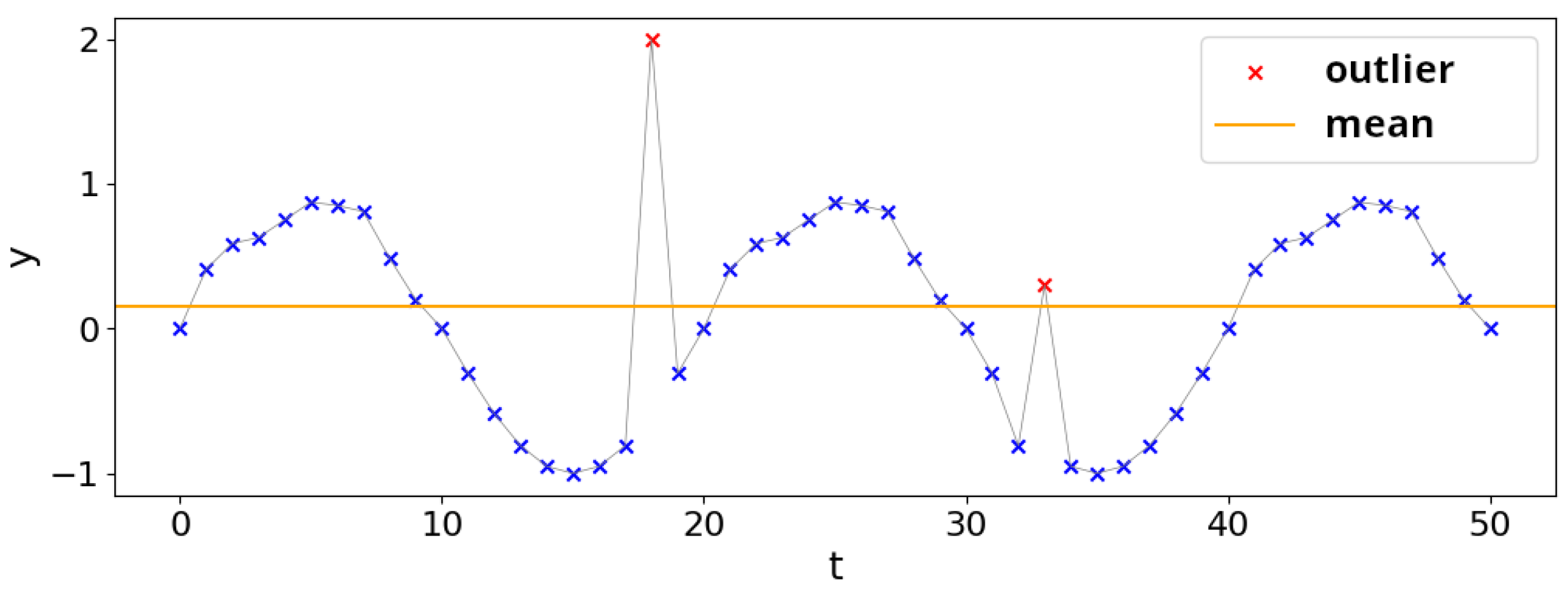
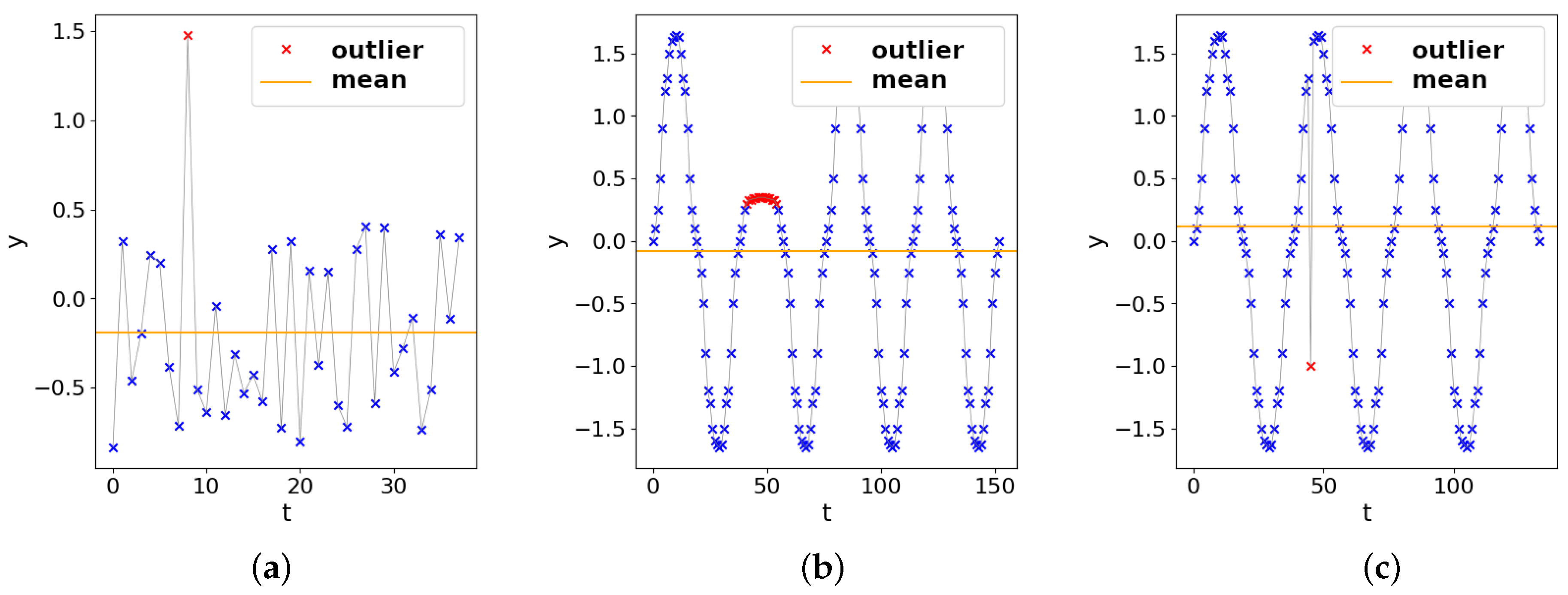
3.2. Outliers and Anomalies
3.3. Implemented and Tested Anomaly Detection Methods
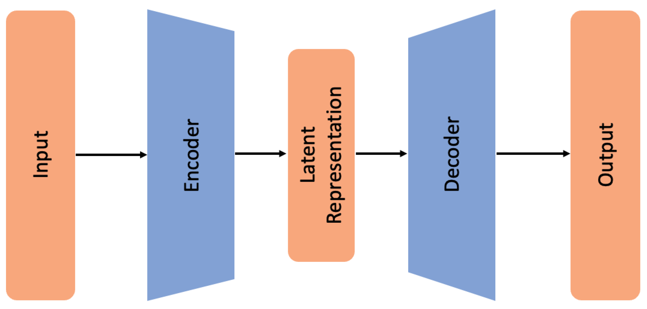
3.3.1. Autoencoder
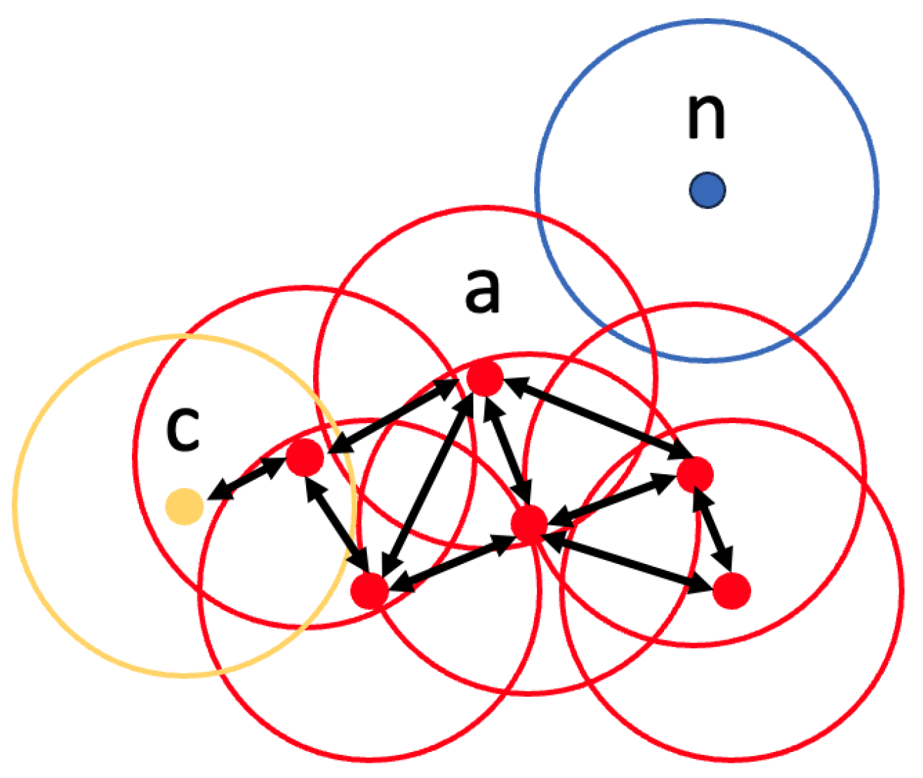
3.3.2. DBSCAN
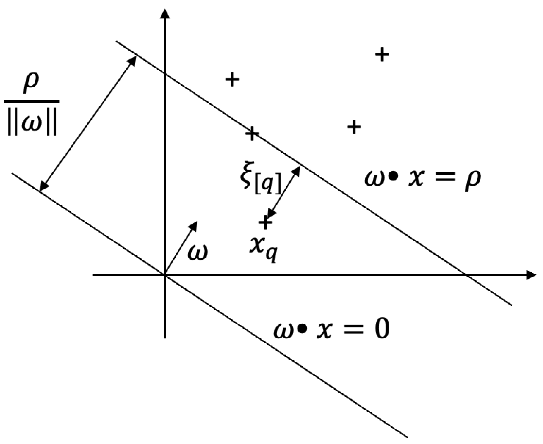
3.3.3. One-Class Support Vector Machine (OCSVM)
3.3.4. Isolation Forest
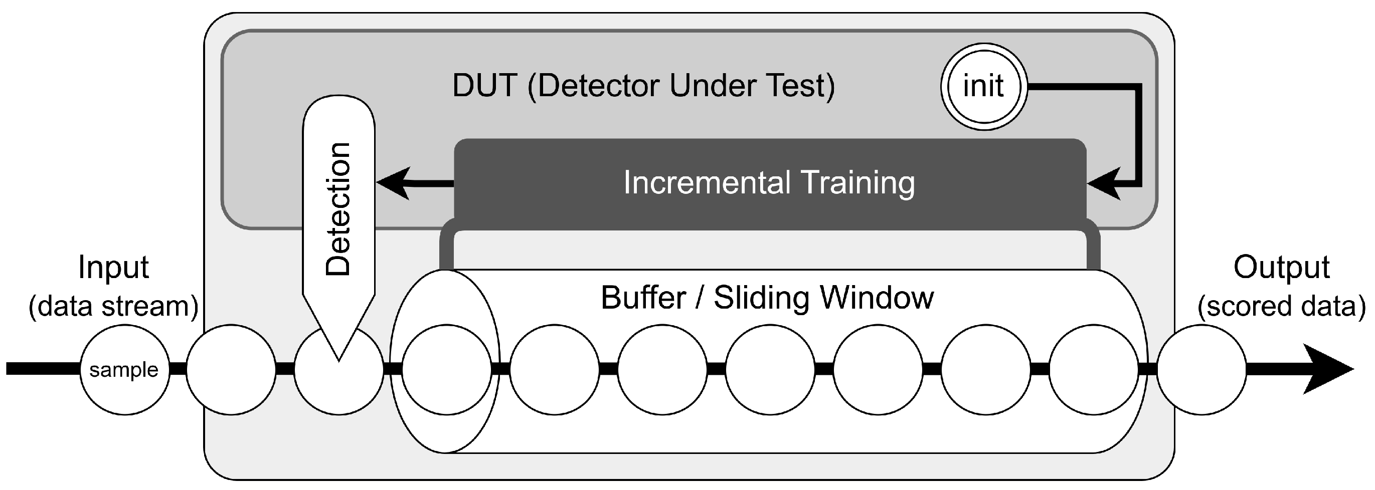
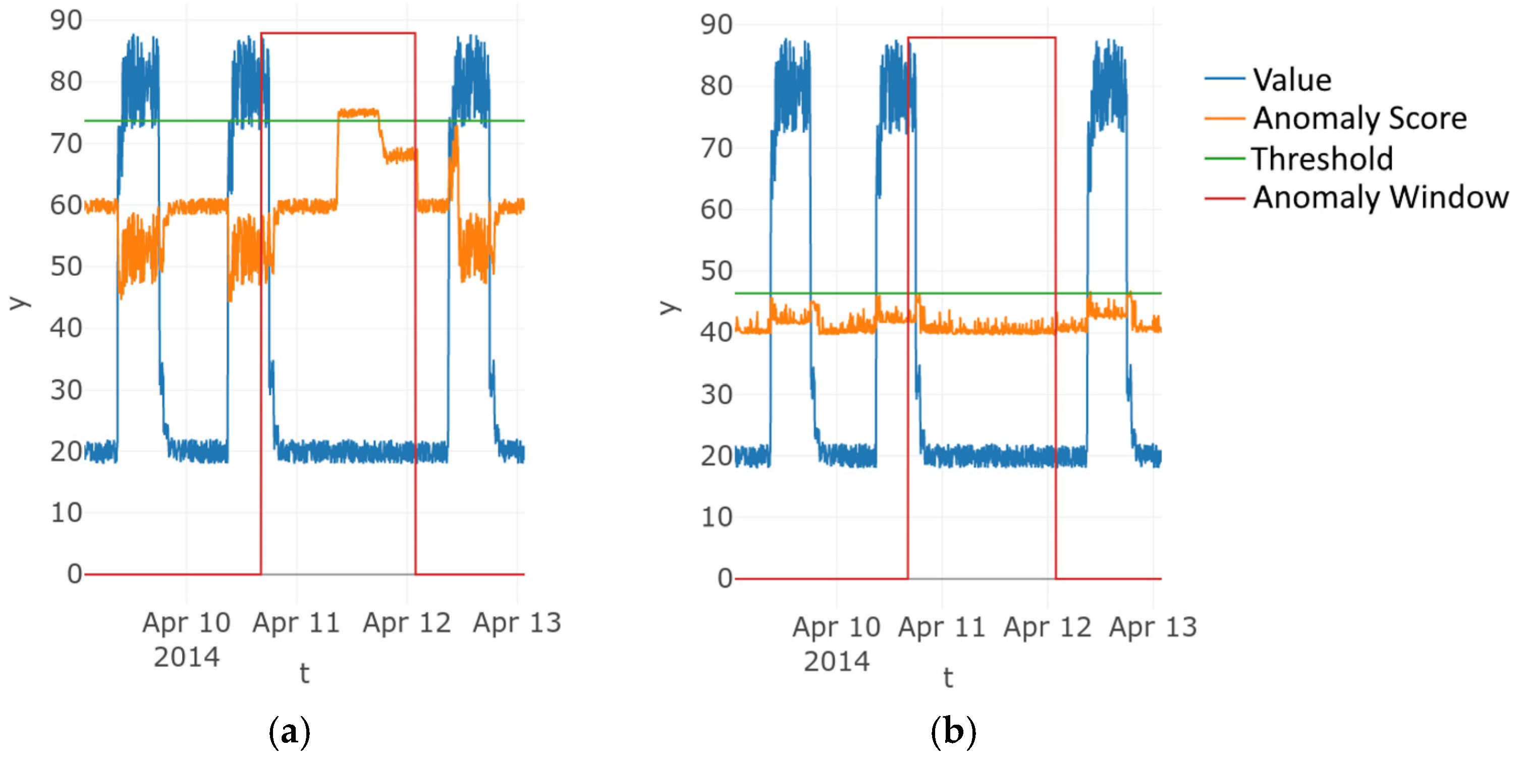
3.4. Numenta-Anomaly-Benchmark (NAB)
- Detection of all anomalies;
- Detection speed;
- No false alarms;
- Detection in real-time (no looking ahead);
- Automation [4] (pp. 39–40).

| Technique | Parameter | Value |
|---|---|---|
| Autoencoder 1 | Optimizer | adam |
| Loss function | mse | |
| DBSCAN | ||
| according to [45] | ||
| iForest | t | 100 |
| 256 | ||
| Contamination | ||
| OCSVM | Kernel Function | rbf |
4. Results
4.1. Correctness
4.2. Distinctiveness
4.3. Robustness
4.4. Outcome of the Individual Anomaly Detection Methods
4.5. Autoencoder
4.6. DBSCAN
4.7. One-Class Support Vector Machine (OCSVM)
4.8. Isolation Forest
4.9. Summary
5. Conclusions
Author Contributions
Funding
Data Availability Statement
Acknowledgments
Conflicts of Interest
References
- Schäfer, F.; Mayr, A.; Schwulera, E.; Franke, J. Smart Use Case Picking with DUCAR: A Hands-On Approach for a Successful Integration of Machine Learning in Production Processes. Procedia Manuf. 2020, 51, 1311–1318. [Google Scholar] [CrossRef]
- Singh, K.; Upadhyaya, S. Outlier detection: Applications and techniques. Int. J. Comput. Sci. Issues (IJCSI) 2012, 9, 307–323. [Google Scholar]
- Schindler, T.F.; Bode, D.; Thoben, K.D. Towards Challenges and Proposals for Integrating and Using Machine Learning Methods in Production Environments. In Proceedings of the International Conference on System-Integrated Intelligence, Genova, Italy, 7–9 September 2022; Springer: Berlin/Heidelberg, Germany, 2022; pp. 3–12. [Google Scholar]
- Lavin, A.; Ahmad, S. Evaluating Real-Time Anomaly Detection Algorithms – The Numenta Anomaly Benchmark. In Proceedings of the 2015 IEEE 14th International Conference on Machine Learning and Applications (ICMLA), Miami, FL, USA, 9–11 December 2015. [Google Scholar] [CrossRef]
- Freeman, C.; Merriman, J.; Beavers, I.; Mueen, A. Experimental Comparison of Online Anomaly Detection Algorithms. In Proceedings of the Thirty-Second International Flairs Conference, Sarasota, FL, USA, 19–22 May 2019. [Google Scholar]
- Maciąg, P.S.; Kryszkiewicz, M.; Bembenik, R.; Lobo, J.L.; Del Ser, J. Unsupervised Anomaly Detection in Stream Data with Online Evolving Spiking Neural Networks. Neural Netw. 2021, 139, 118–139. [Google Scholar] [CrossRef] [PubMed]
- Nassif, A.B.; Talib, M.A.; Nasir, Q.; Dakalbab, F.M. Machine learning for anomaly detection: A systematic review. IEEE Access 2021, 9, 78658–78700. [Google Scholar] [CrossRef]
- Wan, F.; Guo, G.; Zhang, C.; Guo, Q.; Liu, J. Outlier Detection for Monitoring Data Using Stacked Autoencoder. IEEE Access 2019, 7, 173827–173837. [Google Scholar] [CrossRef]
- Ahmad, S.; Styp-Rekowski, K.; Nedelkoski, S.; Kao, O. Autoencoder-based Condition Monitoring and Anomaly Detection Method for Rotating Machines. In Proceedings of the 2020 IEEE International Conference on Big Data (Big Data), Atlanta, GA, USA, 10–13 December 2020. [Google Scholar] [CrossRef]
- Hussain, M.; Ali, N.; Hong, J.E. DeepGuard: A framework for safeguarding autonomous driving systems from inconsistent behaviour. Autom. Softw. Eng. 2021, 29, 1. [Google Scholar] [CrossRef]
- Stocco, A.; Tonella, P. Towards Anomaly Detectors that Learn Continuously. In Proceedings of the 2020 IEEE International Symposium on Software Reliability Engineering Workshops (ISSREW), Coimbra, Portugal, 12–15 October 2020. [Google Scholar] [CrossRef]
- Hussain, M.; Suh, J.W.; Seo, B.S.; Hong, J.E. How Reliable are the Deep Learning-based Anomaly Detectors? A Comprehensive Reliability Analysis of Autoencoder-based Anomaly Detectors. In Proceedings of the 2023 Fourteenth International Conference on Ubiquitous and Future Networks (ICUFN), Paris, France, 4–7 July 2023. [Google Scholar] [CrossRef]
- Celik, M.; Dadaser-Celik, F.; Dokuz, A.S. Anomaly detection in temperature data using DBSCAN algorithm. In Proceedings of the 2011 International Symposium on Innovations in Intelligent Systems and Applications, Istanbul, Turkey, 15–18 June 2011. [Google Scholar] [CrossRef]
- Ijaz, M.; Alfian, G.; Syafrudin, M.; Rhee, J. Hybrid Prediction Model for Type 2 Diabetes and Hypertension Using DBSCAN-Based Outlier Detection, Synthetic Minority Over Sampling Technique (SMOTE), and Random Forest. Appl. Sci. 2018, 8, 1325. [Google Scholar] [CrossRef]
- Sheridan, K.; Puranik, T.G.; Mangortey, E.; Pinon-Fischer, O.J.; Kirby, M.; Mavris, D.N. An Application of DBSCAN Clustering for Flight Anomaly Detection During the Approach Phase. In Proceedings of the AIAA Scitech 2020 Forum, Orlando, FL, USA, 6–10 January 2020. [Google Scholar] [CrossRef]
- John, H.; Naaz, S. Credit Card Fraud Detection using Local Outlier Factor and Isolation Forest. Int. J. Comput. Sci. Eng. 2019, 7, 1060–1064. [Google Scholar] [CrossRef]
- Khaledian, E.; Pandey, S.; Kundu, P.; Srivastava, A.K. Real-Time Synchrophasor Data Anomaly Detection and Classification Using Isolation Forest, KMeans, and LoOP. IEEE Trans. Smart Grid 2021, 12, 2378–2388. [Google Scholar] [CrossRef]
- Ripan, R.C.; Sarker, I.H.; Anwar, M.M.; Furhad, M.H.; Rahat, F.; Hoque, M.M.; Sarfraz, M. An Isolation Forest Learning Based Outlier Detection Approach for Effectively Classifying Cyber Anomalies. In Advances in Intelligent Systems and Computing; Springer International Publishing: Berlin/Heidelberg, Germany, 2021; pp. 270–279. [Google Scholar] [CrossRef]
- Mourão-Miranda, J.; Hardoon, D.R.; Hahn, T.; Marquand, A.F.; Williams, S.C.; Shawe-Taylor, J.; Brammer, M. Patient classification as an outlier detection problem: An application of the One-Class Support Vector Machine. NeuroImage 2011, 58, 793–804. [Google Scholar] [CrossRef]
- Shia, H.H.; Ali Tawfeeq, M.; Mahmoud, S.M. High Rate Outlier Detection in Wireless Sensor Networks: A Comparative Study. Int. J. Mod. Educ. Comput. Sci. 2019, 11, 13–22. [Google Scholar] [CrossRef]
- Wang, Z.; Fu, Y.; Song, C.; Zeng, P.; Qiao, L. Power System Anomaly Detection Based on OCSVM Optimized by Improved Particle Swarm Optimization. IEEE Access 2019, 7, 181580–181588. [Google Scholar] [CrossRef]
- Yang, K.; Kpotufe, S.; Feamster, N. An Efficient One-Class SVM for Anomaly Detection in the Internet of Things. arXiv 2021, arXiv:2104.11146. [Google Scholar] [CrossRef]
- Mockenhaupt, A. Digitalisierung und Künstliche Intelligenz in der Produktion; Springer: Wiesbaden, Germany, 2021. [Google Scholar] [CrossRef]
- O’Leary, D.E. Artificial intelligence and big data. IEEE Intell. Syst. 2013, 28, 96–99. [Google Scholar] [CrossRef]
- Runkler, T.A. Data Mining: Modelle und Algorithmen Intelligenter Datenanalyse, 2nd ed.; Computational Intelligence; Springer: Wiesbaden, Germany, 2015. [Google Scholar]
- Mehrotra, K.G.; Mohan, C.K.; Huang, H. Anomaly Detection Principles and Algorithms; Springer: Berlin/Heidelberg, Germany, 2017; Volume 1. [Google Scholar]
- Hawkins, D.M. Identification of Outliers; Springer: Berlin/Heidelberg, Germany, 1980; Volume 11. [Google Scholar]
- Collett, D.; Lewis, T. The subjective nature of outlier rejection procedures. J. R. Stat. Soc. Ser. C Appl. Stat. 1976, 25, 228–237. [Google Scholar] [CrossRef]
- Aggarwal, C.C. Applications of Outlier Analysis. In Outlier Analysis; Springer International Publishing: Cham, Switzerland, 2017; pp. 399–422. [Google Scholar] [CrossRef]
- Omar, S.; Ngadi, A.; Jebur, H.H. Machine learning techniques for anomaly detection: An overview. Int. J. Comput. Appl. 2013, 79, 33–41. [Google Scholar] [CrossRef]
- Zimek, A.; Filzmoser, P. There and back again: Outlier detection between statistical reasoning and data mining algorithms. Wiley Interdiscip. Rev. Data Min. Knowl. Discov. 2018, 8, e1280. [Google Scholar] [CrossRef]
- Chen, Z.; Yeo, C.K.; Lee, B.S.; Lau, C.T. Autoencoder-based network anomaly detection. In Proceedings of the 2018 Wireless Telecommunications Symposium (WTS), Phoenix, AZ, USA, 17–20 April 2018; pp. 1–5. [Google Scholar]
- Ye, A.; Wang, Z. Autoencoders. In Modern Deep Learning for Tabular Data: Novel Approaches to Common Modeling Problems; Apress: Berkeley, CA, USA, 2023; pp. 601–680. [Google Scholar] [CrossRef]
- Zhou, C.; Paffenroth, R.C. Anomaly detection with robust deep autoencoders. In Proceedings of the 23rd ACM SIGKDD International Conference on Knowledge Discovery and Data Mining, Halifax, NS, Canada, 13–17 August 2017; pp. 665–674. [Google Scholar]
- Ester, M.; Kriegel, H.P.; Sander, J.; Xu, X. A density-based algorithm for discovering clusters in large spatial databases with noise. In Proceedings of the 2nd International Conference on Knowledge Discovery and Data Mining (KDD-96), Portland, OR, USA, 2–4 August 1996; Volume 96, pp. 226–231. [Google Scholar]
- Wibisono, S.; Anwar, M.; Supriyanto, A.; Amin, I. Multivariate weather anomaly detection using DBSCAN clustering algorithm. Proc. J. Phys. Conf. Ser. 2021, 1869, 012077. [Google Scholar] [CrossRef]
- Schubert, E.; Sander, J.; Ester, M.; Kriegel, H.P.; Xu, X. DBSCAN Revisited, Revisited: Why and How You Should (Still) Use DBSCAN. ACM Trans. Database Syst. 2017, 42, 1–21. [Google Scholar] [CrossRef]
- Hejazi, M.; Singh, Y.P. One-class support vector machines approach to anomaly detection. Appl. Artif. Intell. 2013, 27, 351–366. [Google Scholar] [CrossRef]
- Hamel, L.H. Knowledge Discovery with Support Vector Machines; John Wiley & Sons: Hoboken, NJ, USA, 2011; pp. 103–113, 209–217. [Google Scholar]
- Liu, F.T.; Ting, K.M.; Zhou, Z.H. Isolation Forest. In Proceedings of the 2008 Eighth IEEE International Conference on Data Mining, Pisa, Italy, 15–19 December 2008; pp. 413–422. [Google Scholar] [CrossRef]
- Hota, H.; Handa, R.; Shrivas, A.K. Time series data prediction using sliding window based RBF neural network. Int. J. Comput. Intell. Res. 2017, 13, 1145–1156. [Google Scholar]
- Fahrmeir, L.; Heumann, C.; Künstler, R.; Pigeot, I.; Tutz, G. Stetige Zufallsvariablen. In Statistik: Der Weg zur Datenanalyse; Springer: Berlin/Heidelberg, Germany, 2016; pp. 251–287. [Google Scholar] [CrossRef]
- Keras. 2015. Available online: https://keras.io (accessed on 1 December 2023).
- Sander, J.; Ester, M.; Kriegel, H.P.; Xu, X. Density-based clustering in spatial databases: The algorithm gdbscan and its applications. Data Min. Knowl. Discov. 1998, 2, 169–194. [Google Scholar] [CrossRef]
- Akbari, Z.; Unland, R. Automated determination of the input parameter of DBSCAN based on outlier detection. In Proceedings of the Artificial Intelligence Applications and Innovations: 12th IFIP WG 12.5 International Conference and Workshops, AIAI 2016, Thessaloniki, Greece, 16–18 September 2016; Proceedings 12. Springer: Berlin/Heidelberg, Germany, 2016; pp. 280–291. [Google Scholar]
- Pedregosa, F.; Varoquaux, G.; Gramfort, A.; Michel, V.; Thirion, B.; Grisel, O.; Blondel, M.; Prettenhofer, P.; Weiss, R.; Dubourg, V.; et al. Scikit-learn: Machine Learning in Python. J. Mach. Learn. Res. 2011, 12, 2825–2830. [Google Scholar]
- Campos, G.O.; Zimek, A.; Sander, J.; Campello, R.J.; Micenková, B.; Schubert, E.; Assent, I.; Houle, M.E. On the evaluation of unsupervised outlier detection: Measures, datasets, and an empirical study. Data Min. Knowl. Discov. 2016, 30, 891–927. [Google Scholar] [CrossRef]


| Technique | Categorization in Machine Learning |
|---|---|
| Autoencoder | Dimensionality reduction |
| DBSCAN | Clustering |
| Isolation Forest | Hybrid |
| One-Class Support Vector Machine | Classification |
| Detection Result | Outlier (Positive) | No Outlier (Negative) |
|---|---|---|
| Outlier detected | True Positive (TP) | False Positive (FP) |
| Outlier not detected | False Negative (FN) | True Negative (TN) |
| Autoencoder | DBSCAN | iForest | OCSVM | |||||
|---|---|---|---|---|---|---|---|---|
| Dataset | AUC | AUC | AUC | AUC | ||||
| 1 | 40.210 | 0.474 | 93.030 | 0.580 | 99.670 | 0.820 | 93.030 | 0.634 |
| 2 | 42.900 | 0.766 | 93.030 | 0.617 | 55.710 | 0.611 | 93.030 | 0.659 |
| 3 | 93.030 | 0.773 | 93.030 | 0.675 | 59.640 | 0.697 | 93.030 | 0.670 |
| 4 | 93.030 | 0.837 | 0.000 | 0.578 | 34.640 | 0.380 | 0.000 | 0.553 |
| 5 | 0.000 | 0.564 | 0.000 | 0.583 | 0.000 | 0.587 | 0.000 | 0.543 |
| 6 | 87.190 | 0.669 | 86.440 | 0.595 | 92.270 | 0.779 | 97.740 | 0.484 |
| Mean | 59.393 | 0.681 | 60.922 | 0.605 | 56.988 | 0.646 | 62.805 | 0.591 |
| 7 | 46.660 | 0.682 | 91.450 | 0.586 | 0.000 | 0.583 | 47.540 | 0.581 |
| 8 | 0.000 | 0.722 | 98.560 | 0.533 | 0.000 | 0.746 | 98.720 | 0.639 |
| 9 | 95.310 | 0.591 | 83.930 | 0.592 | 67.970 | 0.578 | 80.770 | 0.621 |
| 10 | 48.380 | 0.885 | 41.450 | 0.569 | 0.000 | 0.840 | 0.170 | 0.638 |
| 11 | 53.110 | 0.608 | 16.440 | 0.550 | 0.000 | 0.591 | 0.000 | 0.464 |
| 12 | 0.000 | — | 18.390 | 0.597 | 22.740 | 0.610 | 23.980 | 0.721 |
| 13 | 39.890 | 0.699 | 57.840 | 0.578 | 64.640 | 0.742 | 73.540 | 0.791 |
| Mean | 40.479 | 0.698 | 58.294 | 0.572 | 22.193 | 0.670 | 46.389 | 0.636 |
Disclaimer/Publisher’s Note: The statements, opinions and data contained in all publications are solely those of the individual author(s) and contributor(s) and not of MDPI and/or the editor(s). MDPI and/or the editor(s) disclaim responsibility for any injury to people or property resulting from any ideas, methods, instructions or products referred to in the content. |
© 2023 by the authors. Licensee MDPI, Basel, Switzerland. This article is an open access article distributed under the terms and conditions of the Creative Commons Attribution (CC BY) license (https://creativecommons.org/licenses/by/4.0/).
Share and Cite
Schindler, T.F.; Schlicht, S.; Thoben, K.-D. Towards Benchmarking for Evaluating Machine Learning Methods in Detecting Outliers in Process Datasets. Computers 2023, 12, 253. https://doi.org/10.3390/computers12120253
Schindler TF, Schlicht S, Thoben K-D. Towards Benchmarking for Evaluating Machine Learning Methods in Detecting Outliers in Process Datasets. Computers. 2023; 12(12):253. https://doi.org/10.3390/computers12120253
Chicago/Turabian StyleSchindler, Thimo F., Simon Schlicht, and Klaus-Dieter Thoben. 2023. "Towards Benchmarking for Evaluating Machine Learning Methods in Detecting Outliers in Process Datasets" Computers 12, no. 12: 253. https://doi.org/10.3390/computers12120253