
Diagnosing Ovarian Cancer on MRI: A Preliminary Study Comparing Deep Learning and Radiologist Assessments

 , ,
, ,
Abstract
:Simple Summary
Abstract
1. Introduction
2. Materials and Methods
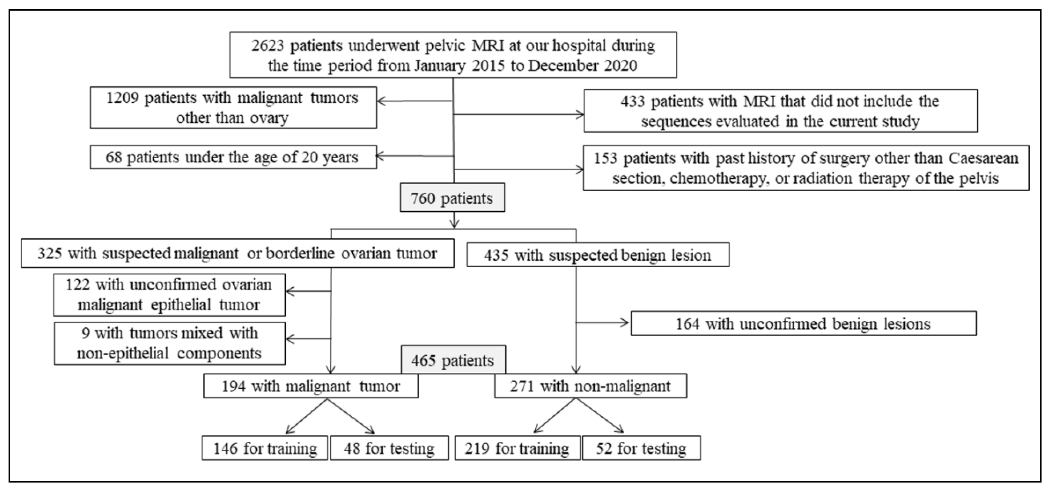
2.1. Patients
2.2. MRI Acquisition
2.3. Data Set
2.4. Deep Learning Using CNNs
2.5. Radiologist Interpretation
2.6. Statistical Analysis
3. Results
4. Discussion
5. Conclusions
Author Contributions
Funding
Institutional Review Board Statement
Informed Consent Statement
Data Availability Statement
Conflicts of Interest
References
- Sung, H.; Ferlay, J.; Siegel, R.L.; Laversanne, M.; Soerjomataram, I.; Jemal, A.; Bray, F. Global Cancer Statistics 2020: GLOBOCAN Estimates of Incidence and Mortality Worldwide for 36 Cancers in 185 Countries. CA Cancer J. Clin. 2021, 71, 209–249. [Google Scholar] [CrossRef]
- Goff, B.A.; Mandel, L.S.; Melancon, C.H.; Muntz, H.G. Frequency of symptoms of ovarian cancer in women presenting to primary care clinics. JAMA 2004, 291, 2705–2712. [Google Scholar] [CrossRef] [Green Version]
- Timmerman, D.; Schwärzler, P.; Collins, W.P.; Claerhout, F.; Coenen, M.; Amant, F.; Vergote, I.; Bourne, T. Subjective assessment of adnexal masses with the use of ultrasonography: An analysis of interobserver variability and experience. Ultrasound Obstet. Gynecol. 1999, 13, 11–16. [Google Scholar] [CrossRef]
- Sadowski, E.A.; Rockall, A.G.; Maturen, K.E.; Robbins, J.B.; Thomassin-Naggara, I. Adnexal lesions: Imaging strategies for ultrasound and MR imaging. Diagn. Interv. Imaging 2019, 100, 635–646. [Google Scholar] [CrossRef]
- Rieber, A.; Nüssle, K.; Stöhr, I.; Grab, D.; Fenchel, S.; Kreienberg, R.; Reske, S.N.; Brambs, H.J. Preoperative diagnosis of ovarian tumors with MR imaging: Comparison with transvaginal sonography, positron emission tomography, and histologic findings. Am. J. Roentgenol. 2001, 177, 123–129. [Google Scholar] [CrossRef]
- Hricak, H.; Chen, M.; Coakley, F.V.; Kinkel, K.; Yu, K.K.; Sica, G.; Bacchetti, P.; Powell, C.B. Complex Adnexal Masses: Detection and Characterization with MR Imaging—Multivariate Analysis. Radiology 2000, 214, 39–46. [Google Scholar] [CrossRef]
- Pi, S.; Cao, R.; Qiang, J.W.; Guo, Y.H. Utility of DWI with quantitative ADC values in ovarian tumors: A meta-analysis of diagnostic test performance. Acta Radiol. 2018, 59, 1386–1394. [Google Scholar] [CrossRef]
- Fujii, S.; Kakite, S.; Nishihara, K.; Kanasaki, Y.; Harada, T.; Kigawa, J.; Kaminou, T.; Ogawa, T. Diagnostic accuracy of diffusion-weighted imaging in differentiating benign from malignant ovarian lesions. J. Magn. Reson. Imaging 2008, 28, 1149–1156. [Google Scholar] [CrossRef]
- Ricke, J.; Sehouli, J.; Hach, C.; Hänninen, E.L.; Lichtenegger, W.; Felix, R. Prospective evaluation of contrast-enhanced MRI in the depiction of peritoneal spread in primary or recurrent ovarian cancer. Eur. Radiol. 2003, 13, 943–949. [Google Scholar] [CrossRef]
- Thomassin-Naggara, I.; Aubert, E.; Rockall, A.; Jalaguier-Coudray, A.; Rouzier, R.; Daraï, E.; Bazot, M. Adnexal Masses: Development and Preliminary Validation of an MR Imaging Scoring System. Radiology 2013, 267, 432–443. [Google Scholar] [CrossRef]
- Park, S.Y.; Oh, Y.T.; Jung, D.C. Differentiation between borderline and benign ovarian tumors: Combined analysis of MRI with tumor markers for large cystic masses (≥5 cm). Acta Radiol. 2015, 57, 633–639. [Google Scholar] [CrossRef]
- Soffer, S.; Ben-Cohen, A.; Shimon, O.; Amitai, M.M.; Greenspan, H.; Klang, E. Convolutional Neural Networks for Radiologic Images: A Radiologist’s Guide. Radiology 2019, 290, 590–606. [Google Scholar] [CrossRef]
- Chollet, F. Xception: Deep learning with depthwise separa-ble convolutions. In Proceedings of the IEEE Conference on Computer Vision and Pattern Recognition, Honolulu, HI, USA, 21–26 July 2017. [Google Scholar]
- Russakovsky, O.; Deng, J.; Su, H.; Krause, J.; Satheesh, S.; Ma, S.; Huang, Z.; Karpathy, A.; Khosla, A.; Bernstein, M.; et al. ImageNet Large Scale Visual Recognition Challenge. Int. J. Comput. Vis. 2015, 115, 211–252. [Google Scholar] [CrossRef] [Green Version]
- Linden, A. Measuring diagnostic and predictive accuracy in disease management: An introduction to receiver operating characteristic (ROC) analysis. J. Eval. Clin. Pract. 2006, 12, 132–139. [Google Scholar] [CrossRef]
- Landis, J.R.; Koch, G.G. The Measurement of Observer Agreement for Categorical Data. Biometrics 1977, 33, 159–174. [Google Scholar] [CrossRef] [Green Version]
- Urushibara, A.; Saida, T.; Mori, K.; Ishiguro, T.; Sakai, M.; Masuoka, S.; Satoh, T.; Masumoto, T. Diagnosing uterine cervical cancer on a single T2-weighted image: Comparison between deep learning versus radiologists. Eur. J. Radiol. 2021, 135, 109471. [Google Scholar] [CrossRef]
- Aramendía-Vidaurreta, V.; Cabeza, R.; Villanueva, A.; Navallas, J.; Alcázar, J.L. Ultrasound Image Discrimination between Benign and Malignant Adnexal Masses Based on a Neural Network Approach. Ultrasound Med. Biol. 2016, 42, 742–752. [Google Scholar] [CrossRef]
- Jian, J.; Li, Y.A.; Pickhardt, P.J.; Xia, W.; He, Z.; Zhang, R.; Zhao, S.; Zhao, X.; Cai, S.; Zhang, J.; et al. MR image-based radiomics to differentiate type Ι and type ΙΙ epithelial ovarian cancers. Eur. Radiol. 2021, 3, 403–410. [Google Scholar] [CrossRef]
- Li, Y.; Jian, J.; Pickhardt, P.J.; Ma, F.; Xia, W.; Li, H.; Zhang, R.; Zhao, S.; Cai, S.; Zhao, X.; et al. MRI-Based Machine Learning for Differentiating Borderline from Malignant Epithelial Ovarian Tumors: A Multicenter Study. J. Magn. Reson. Imaging 2020, 52, 897–904. [Google Scholar] [CrossRef]
- Wang, R.; Cai, Y.; Lee, I.K.; Hu, R.; Purkayastha, S.; Pan, I.; Yi, T.; Tran, T.M.L.; Lu, S.; Liu, T.; et al. Evaluation of a convolutional neural network for ovarian tumor differentiation based on magnetic resonance imaging. Eur. Radiol. 2021, 31, 4960–4971. [Google Scholar] [CrossRef]
- WHO Classification of Tumours Editorial Board. Female Genital Tumours WHO Classification of Tumours, 5th ed.; World Health Organization: Lyon, France, 2020; pp. 32–76. [Google Scholar]
- Tanaka, Y.O.; Okada, S.; Satoh, T.; Matsumoto, K.; Oki, A.; Saida, T.; Yoshikawa, H.; Minami, M. Differentiation of epithelial ovarian cancer subtypes by use of imaging and clinical data: A detailed analysis. Cancer Imaging 2016, 16, 3. [Google Scholar] [CrossRef] [Green Version]
- Foti, P.V.; Attinà, G.; Spadola, S.; Caltabiano, R.; Farina, R.; Palmucci, S.; Zarbo, G.; Zarbo, R.; D’Arrigo, M.; Milone, P.; et al. MR imaging of ovarian masses: Classification and differential diagnosis. Insights Imaging 2016, 7, 21–41. [Google Scholar] [CrossRef] [Green Version]
- Ando, T.; Kato, H.; Kawaguchi, M.; Furui, T.; Morishige, K.I.; Hyodo, F.; Matsuo, M. MR findings for differentiating decidualized endometriomas from seromucinousborderline tumors of the ovary. Abdom. Radiol. 2020, 45, 1783–1789. [Google Scholar] [CrossRef]
- Laurent, P.-E.; Thomassin-Piana, J.; Jalaguier-Coudray, A. Mucin-producing tumors of the ovary: MR imaging appearance. Diagn. Interv. Imaging 2015, 96, 1125–1132. [Google Scholar] [CrossRef] [Green Version]
- Marko, J.; Marko, K.I.; Pachigolla, S.L.; Crothers, B.A.; Mattu, R.; Wolf-Man, D.J. Mucinous neoplasms of the ovary: Radiologic-patho- logic correlation. Radiographics 2019, 39, 982–997. [Google Scholar] [CrossRef]
- Aldoj, N.; Lukas, S.; Dewey, S.M.; Penzkofer, T. Semi-automatic classification of prostate cancer on multi-parametric MR imaging using a multi-channel 3D convolutional neural network. Eur. Radiol. 2020, 30, 1243–1253. [Google Scholar] [CrossRef]
- Le, M.H.; Chen, J.; Wang, L.; Wang, Z.; Liu, W.; Cheng, K.T.; Yang, X. Automated diagnosis of prostate cancer in multi-parametric MRI based on multimodal convolutional neural networks. Phys. Med. Biol. 2017, 62, 6497–6514. [Google Scholar] [CrossRef]
- Wang, X.; Peng, Y.; Lu, L.; Lu, Z.; Bagheri, M.; Summers, R.M. ChestX-Ray8: Hospital-Scale Chest X-Ray Database and Benchmarks on Weakly-Supervised Classification and Localization of Common Thorax Diseases. In Proceedings of the IEEE Conference on Computer Vision and Pattern Recognition, Honolulu, HI, USA, 21–26 July 2017; pp. 2097–2106. [Google Scholar]


| Sequence | Type | Repetition Time/Echo Time (ms) | Flip Angle (Degree) | Slice/Gap (mm) | Field of View (mm) | Matrix |
|---|---|---|---|---|---|---|
| T2WI | 2D Turbo-spin echo | 1400–6013/10–110 | 90 | 3–5/0.3–1 | 260–380 | 512 × 512–704 × 704 |
| DWI | Echo planar imaging | 4068–7500/70–79 | 90 | 3–5/0–1 | 260–380 | 224 × 224–352 × 352 |
| CE-T1WI | 3D Gradient echo spectral pre-saturation with inversion recovery | 4–5/2 | 10–15 | 2.2–3.3/0–1.6 | 260–380 | 352 × 352–704 × 704 |
| Variable | Training Data | Testing Data | ||||
|---|---|---|---|---|---|---|
| Malignant Group | Non-Malignant Group | All | Malignant Group | Non-Malignant Group | All | |
| Patients (n) | 146 | 219 | 365 | 48 | 52 | 100 |
| Images (slices) | 1798 | 1865 | 3663 | 48 | 52 | 100 |
| Age | ||||||
| Mean ± standard deviation (y) | 55 ± 14 | 47 ± 13 | 50 ± 14 | 55 ± 14 | 45 ± 14 | 50 ± 15 |
| Range (y) | 20–87 | 21–86 | 20–87 | 22–76 | 20–90 | 20–90 |
| Tumor stage of malignant group (n) (I/Ⅱ/Ⅲ/Ⅳ) | 83/17/34/22 | 28/3/14/3 | ||||
| Tumor type of malignant group (n) | ||||||
| Serous tumor (HGSC/LGSC/BOT) | 39/1/5 | 14/0/1 | ||||
| Clear cell tumor (carcinoma/BOT) | 40/0 | 13/0 | ||||
| Mucinous tumor (carcinoma/BOT) | 15/18 | 4/6 | ||||
| Endometrioid tumor (carcinoma/BOT) | 14/4 | 5/2 | ||||
| Seromucinous tumor (carcinoma/BOT) | 4/6 | 1/2 | ||||
| Tumor type of non-malignant group (n) | ||||||
| Serous tumor (cystadenoma/adenofibroma) | 15/6 | 6/1 | ||||
| Mucinous tumor (cystadenoma/adenofibroma) | 34/1 | 10/0 | ||||
| Seromucinous cystadenoma | 2 | 1 | ||||
| Endometriosis | 28 | 7 | ||||
| Mature teratoma | 16 | 6 | ||||
| Leiomyoma | 56 | 10 | ||||
| Uterine benign lesion other than leiomyoma | 39 | 9 | ||||
| Other (including normal) | 22 | 2 | ||||
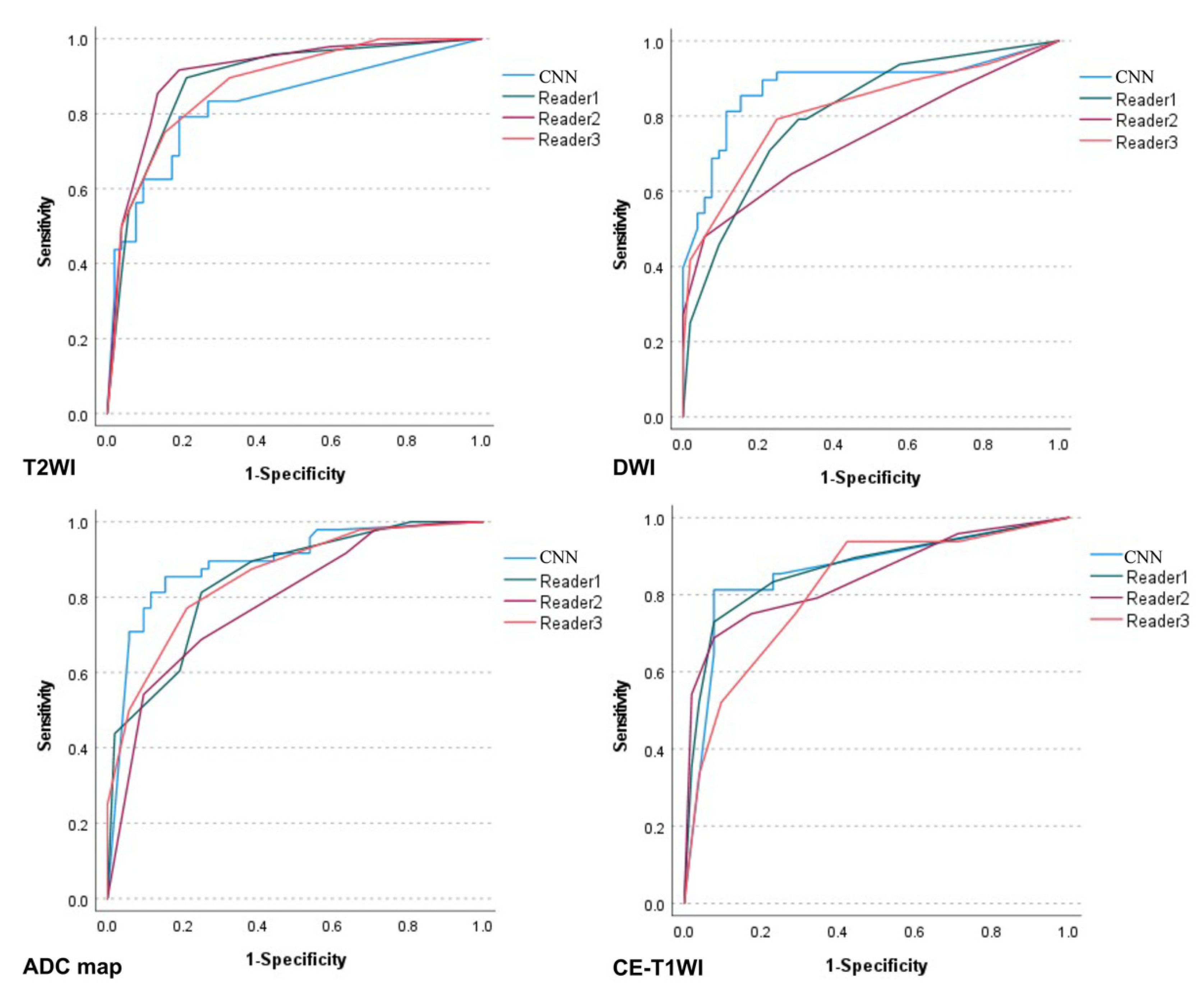
| Sequence | Interpreter | Sensitivity | 95% CI | Specificity | 95% CI | Accuracy | 95% CI | AUC | 95% CI | p-Value for AUC (Versus CNN) |
|---|---|---|---|---|---|---|---|---|---|---|
| T2WI | CNN | 0.77 | 0.68–0.84 | 0.85 | 0.76–0.91 | 0.81 | 0.72–0.87 | 0.83 | 0.74–0.91 | - |
| Reader 1 | 0.63 | 0.54–0.68 | 0.90 | 0.82–0.96 | 0.77 | 0.69–0.82 | 0.89 | 0.82–0.95 | 0.127 | |
| Reader 2 | 0.85 | 0.77–0.91 | 0.87 | 0.79- 0.92 | 0.86 | 0.78–0.92 | 0.91 | 0.85–0.97 | 0.048 * | |
| Reader 3 | 0.75 | 0.66–0.82 | 0.85 | 0.76–0.91 | 0.80 | 0.71–0.86 | 0.88 | 0.81–0.94 | 0.305 | |
| DWI | CNN | 0.85 | 0.77–0.91 | 0.85 | 0.77–0.90 | 0.85 | 0.77–0.91 | 0.88 | 0.81–0.95 | - |
| Reader 1 | 0.71 | 0.61–0.79 | 0.77 | 0.68–0.84 | 0.74 | 0.65–0.82 | 0.81 | 0.72–0.89 | 0.151 | |
| Reader 2 | 0.65 | 0.55–0.73 | 0.71 | 0.62–0.79 | 0.68 | 0.58–0.76 | 0.74 | 0.64–0.84 | 0.004 * | |
| Reader 3 | 0.79 | 0.70–0.87 | 0.75 | 0.66–0.82 | 0.77 | 0.68–0.84 | 0.82 | 0.73–0.90 | 0.135 | |
| ADC map | CNN | 0.85 | 0.76–0.92 | 0.77 | 0.69–0.83 | 0.81 | 0.72–0.87 | 0.89 | 0.83–0.96 | - |
| Reader 1 | 0.81 | 0.72–0.88 | 0.75 | 0.66–0.82 | 0.78 | 0.69–0.85 | 0.84 | 0.77–0.92 | 0.263 | |
| Reader 2 | 0.92 | 0.83–0.97 | 0.36 | 0.29–0.41 | 0.63 | 0.55–0.68 | 0.79 | 0.70–0.88 | 0.023 * | |
| Reader 3 | 0.77 | 0.68–0.84 | 0.79 | 0.70–0.86 | 0.78 | 0.69–0.85 | 0.85 | 0.78–0.93 | 0.356 | |
| CE-T1WI | CNN | 0.81 | 0.73–0.86 | 0.92 | 0.85–0.97 | 0.87 | 0.79–0.92 | 0.86 | 0.78–0.94 | - |
| Reader 1 | 0.73 | 0.65–0.78 | 0.92 | 0.85–0.97 | 0.83 | 0.75- 0.88 | 0.87 | 0.79–0.94 | 0.903 | |
| Reader 2 | 0.75 | 0.66–0.82 | 0.83 | 0.74–0.89 | 0.79 | 0.70–0.86 | 0.85 | 0.77–0.92 | 0.730 | |
| Reader 3 | 0.75 | 0.65–0.83 | 0.71 | 0.62–0.79 | 0.73 | 0.64–0.81 | 0.82 | 0.73–0.90 | 0.416 |
| Comparison | Interpreter | T2WI | DWI | ADC Map | CE-T1WI |
|---|---|---|---|---|---|
| CNN vs. radiologists | 1 | 0.42 | 0.50 | 0.42 | 0.63 |
| 2 | 0.50 | 0.46 | 0.17 | 0.55 | |
| 3 | 0.45 | 0.56 | 0.42 | 0.36 | |
| Between radiologists | 1 vs. 2 | 0.58 | 0.60 | 0.45 | 0.63 |
| 2 vs. 3 | 0.68 | 0.50 | 0.39 | 0.52 | |
| 1 vs. 3 | 0.77 | 0.58 | 0.84 | 0.64 |
Publisher’s Note: MDPI stays neutral with regard to jurisdictional claims in published maps and institutional affiliations. |
© 2022 by the authors. Licensee MDPI, Basel, Switzerland. This article is an open access article distributed under the terms and conditions of the Creative Commons Attribution (CC BY) license (https://creativecommons.org/licenses/by/4.0/).
Share and Cite
Saida, T.; Mori, K.; Hoshiai, S.; Sakai, M.; Urushibara, A.; Ishiguro, T.; Minami, M.; Satoh, T.; Nakajima, T. Diagnosing Ovarian Cancer on MRI: A Preliminary Study Comparing Deep Learning and Radiologist Assessments. Cancers 2022, 14, 987. https://doi.org/10.3390/cancers14040987
Saida T, Mori K, Hoshiai S, Sakai M, Urushibara A, Ishiguro T, Minami M, Satoh T, Nakajima T. Diagnosing Ovarian Cancer on MRI: A Preliminary Study Comparing Deep Learning and Radiologist Assessments. Cancers. 2022; 14(4):987. https://doi.org/10.3390/cancers14040987
Chicago/Turabian StyleSaida, Tsukasa, Kensaku Mori, Sodai Hoshiai, Masafumi Sakai, Aiko Urushibara, Toshitaka Ishiguro, Manabu Minami, Toyomi Satoh, and Takahito Nakajima. 2022. "Diagnosing Ovarian Cancer on MRI: A Preliminary Study Comparing Deep Learning and Radiologist Assessments" Cancers 14, no. 4: 987. https://doi.org/10.3390/cancers14040987