


Deep Learning for Automated Elective Lymph Node Level Segmentation for Head and Neck Cancer Radiotherapy
Abstract
:Simple Summary
Abstract
1. Introduction
2. Materials and Methods
2.1. Data Acquisition
2.2. Pre-Processing
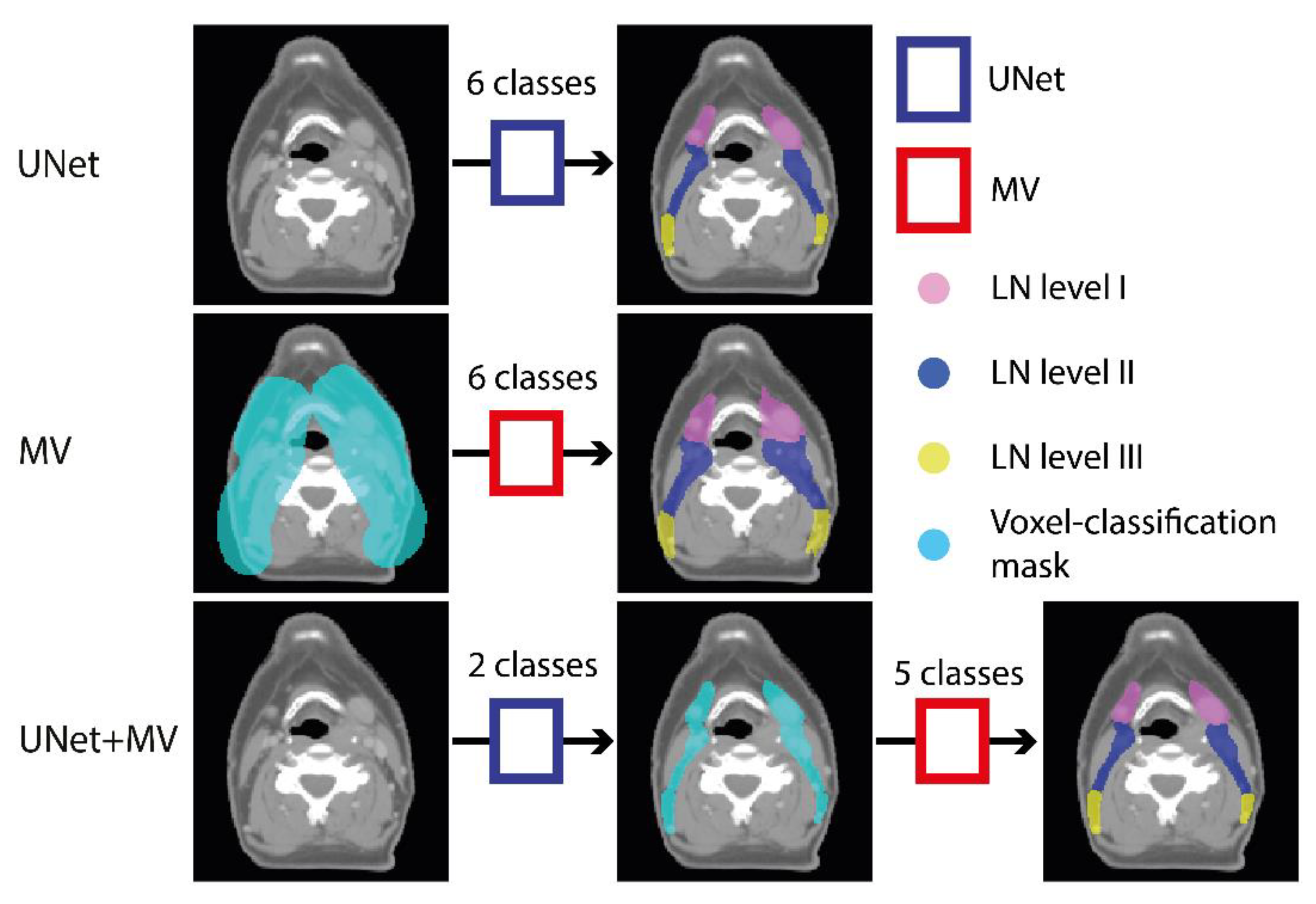
2.3. Experimental Outline
2.4. Model Training
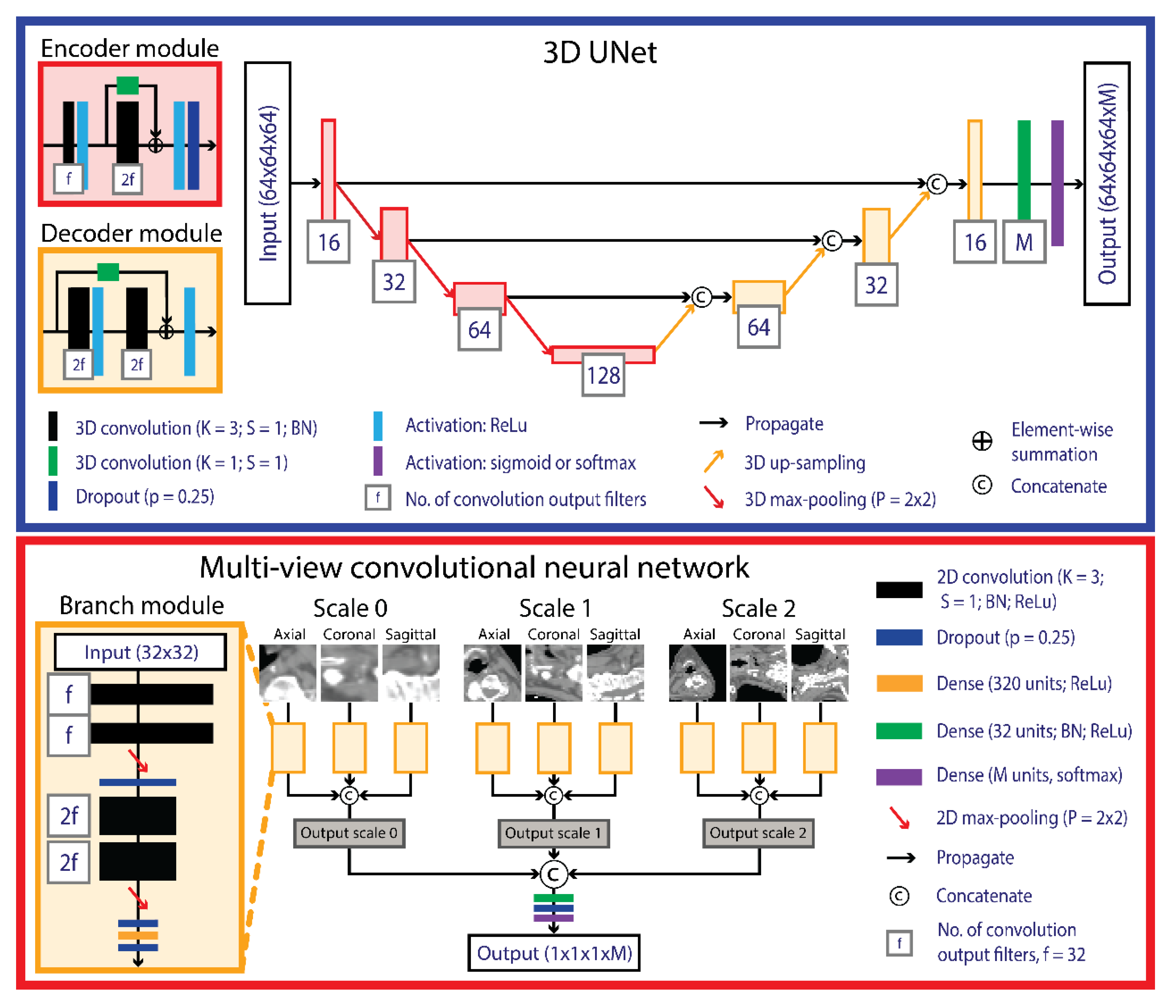
2.4.1. UNet
2.4.2. Multi-View
2.4.3. Data Augmentation
2.5. Post-Processing
2.6. Evaluation and Statistical Analysis
2.7. Independent Validation
3. Results
4. Discussion
5. Conclusions
Supplementary Materials
Author Contributions
Funding
Institutional Review Board Statement
Informed Consent Statement
Data Availability Statement
Conflicts of Interest
References
- Van der Veen, J.; Gulyban, A.; Nuyts, S. Interobserver variability in delineation of target volumes in head and neck cancer. Radiother. Oncol. 2019, 137, 9–15. [Google Scholar] [CrossRef] [PubMed]
- Grégoire, V.; Ang, K.; Budach, W.; Grau, C.; Hamoir, M.; Langendijk, J.A.; Lee, A.; Le, Q.-T.; Maingon, P.; Nutting, C.; et al. Delineation of the primary tumour Clinical Target Volumes (CTV-P) in laryngeal, hypopharyngeal, oropharyngeal and oral cavity squamous cell carcinoma: AIRO, CACA, DAHANCA, EORTC, GEORCC, GORTEC, HKNPCSG, HNCIG, IAG-KHT, LPRHHT, NCIC CTG, NCRI, NRG Oncolog. Int. J. Radiat. Oncol. 2019, 104, 677–684. [Google Scholar] [CrossRef] [Green Version]
- Van Rooij, W.; Dahele, M.; Brandao, H.R.; Delaney, A.R.; Slotman, B.J.; Verbakel, W.F.A.R. Deep Learning-Based Delineation of Head and Neck Organs at Risk: Geometric and Dosimetric Evaluation. Int. J. Radiat. Oncol. 2019, 104, 677–684. [Google Scholar] [CrossRef] [PubMed]
- Zhu, W.; Huang, Y.; Zeng, L.; Chen, X.; Liu, Y.; Qian, Z.; Du, N.; Fan, W.; Xie, X. AnatomyNet: Deep learning for fast and fully automated whole-volume segmentation of head and neck anatomy. Med. Phys. 2018, 46, 576–589. [Google Scholar] [CrossRef] [PubMed] [Green Version]
- Wang, W.; Wang, Q.; Jia, M.; Wang, Z.; Yang, C.; Zhang, D.; Wen, S.; Hou, D.; Liu, N.; Wang, P. Deep Learning-Augmented Head and Neck Organs at Risk Segmentation From CT Volumes. Front. Phys. 2021, 9, 1–11. [Google Scholar] [CrossRef]
- Kawahara, D.; Tsuneda, M.; Ozawa, S.; Okamoto, H.; Nakamura, M.; Nishio, T.; Saito, A.; Nagata, Y. Stepwise deep neural network (stepwise-net) for head and neck auto-segmentation on CT images. Comput. Biol. Med. 2022, 143, 105295. [Google Scholar] [CrossRef]
- Ali, R.; Hardie, R.C.; Narayanan, B.N.; Kebede, T.M. IMNets: Deep Learning Using an Incremental Modular Network Synthesis Approach for Medical Imaging Applications. Appl. Sci. 2022, 12, 5500. [Google Scholar] [CrossRef]
- Men, K.; Chen, X.; Zhang, Y.; Zhang, T.; Dai, J.; Yi, J.; Li, Y. Deep deconvolutional neural network for target segmentation of nasopharyngeal cancer in planning computed tomography images. Front. Oncol. 2017, 7, 315. [Google Scholar] [CrossRef] [Green Version]
- Cardenas, C.E.; Beadle, B.M.; Garden, A.S.; Skinner, H.D.; Yang, J.; Rhee, D.J.; McCarroll, R.E.; Netherton, T.J.; Gay, S.S.; Zhang, L. Generating High-Quality Lymph Node Clinical Target Volumes for Head and Neck Cancer Radiation Therapy Using a Fully Automated Deep Learning-Based Approach. Int. J. Radiat. Oncol. 2021, 109, 801–812. [Google Scholar] [CrossRef]
- Chen, A.; Deeley, M.A.; Niermann, K.J.; Moretti, L.; Dawant, B.M. Combining registration and active shape models for the automatic segmentation of the lymph node regions in head and neck CT images. Med. Phys. 2010, 37, 6338–6346. [Google Scholar] [CrossRef]
- Stapleford, L.J.; Lawson, J.D.; Perkins, C.; Edelman, S.; Davis, L.; McDonald, M.W.; Waller, A.; Schreibmann, E.; Fox, T. Evaluation of Automatic Atlas-Based Lymph Node Segmentation for Head-and-Neck Cancer. Int. J. Radiat. Oncol. 2010, 77, 959–966. [Google Scholar] [CrossRef]
- Ronneberger, O.; Fischer, P.; Brox, T. U-net: Convolutional networks for biomedical image segmentation. In Lecture Notes in Computer Science, Proceedings of the Medical Image Computing and Computer-Assisted Intervention 2015, Munich, Germany, 5–9 October 2015; Springer: Cham, Switzerland, 2015. [Google Scholar] [CrossRef] [Green Version]
- Weissmann, T.; Huang, Y.; Fischer, S.; Roesch, J. Deep Learning for automatic head and neck lymph node level delineation. Int. J. Radiat. Oncol. Biol. Phys. 2022, 1–17. Available online: https://arxiv.org/abs/2208.13224 (accessed on 1 October 2022).
- Van der Veen, J.; Willems, S.; Bollen, H.; Maes, F.; Nuyts, S. Deep learning for elective neck delineation: More consistent and time efficient. Radiother. Oncol. 2020, 153, 180–188. [Google Scholar] [CrossRef]
- Birenbaum, A.; Greenspan, H. Multi-view longitudinal CNN for multiple sclerosis lesion segmentation. Eng. Appl. Artif. Intell. 2017, 65, 111–118. [Google Scholar] [CrossRef]
- Strijbis, V.I.J.; de Bloeme, C.M.; Jansen, R.W.; Kebiri, H.; Nguyen, H.-G.; de Jong, M.C.; Moll, A.C.; Bach-Cuadra, M.; de Graaf, P.; Steenwijk, M.D. Multi-view convolutional neural networks for automated ocular structure and tumor segmentation in retinoblastoma. Sci. Rep. 2021, 11, 14590. [Google Scholar] [CrossRef]
- Roth, H.R.; Lu, L.; Seff, A.; Cherry, K.M.; Hoffman, J.; Wang, S.; Liu, J.; Turkbey, E.; Summers, R.M. A New 2.5D Representation for Lymph Node Detection Using Random Sets of Deep Convolutional Neural Network Observations. In Lecture Notes in Computer Science, Proceedings of the Medical Image Computing and Computer-Assisted Intervention (MICCAI), Boston, MA, USA, 14–18 September 2014; Springer: Cham, Switzerland, 2014; Volume 17, pp. 520–527. [Google Scholar] [CrossRef] [Green Version]
- Schouten, J.P.; Noteboom, S.; Martens, R.M.; Mes, S.W.; Leemans, C.R.; de Graaf, P.; Steenwijk, M.D. Automatic segmentation of head and neck primary tumors on MRI using a multi-view CNN. Cancer Imaging 2022, 22, 8. [Google Scholar] [CrossRef]
- Aslani, S.; Dayan, M.; Storelli, L.; Filippi, M.; Murino, V.; Rocca, M.A.; Sona, D. Multi-branch convolutional neural network for multiple sclerosis lesion segmentation. NeuroImage 2019, 196, 1–15. [Google Scholar] [CrossRef] [Green Version]
- Kingma, D.P.; Ba, J. Adam: A Method for Stochastic Optimization. In Proceedings of the 3rd International Conference of Learning Representations (ICLR), San Diego, USA, 7–9 May 2015. [Google Scholar]
- Ren, J.; Eriksen, J.G.; Nijkamp, J.; Korreman, S.S. Comparing different CT, PET and MRI multi-modality image combinations for deep learning-based head and neck tumor segmentation. Acta Oncol. 2021, 60, 1399–1406. [Google Scholar] [CrossRef]
- Van Rooij, W.; Dahele, M.; Nijhuis, H.; Slotman, B.J.; Verbakel, W.F.A.R. OC-0346: Strategies to improve deep learning-based salivary gland segmentation. Radiat. Oncol. 2020, 15, 272. [Google Scholar] [CrossRef]
- Van Rooij, W.; Verbakel, W.F.; Slotman, B.J.; Dahele, M. Using Spatial Probability Maps to Highlight Potential Inaccuracies in Deep Learning-Based Contours: Facilitating Online Adaptive Radiation Therapy. Adv. Radiat. Oncol. 2021, 6, 100658. [Google Scholar] [CrossRef]
- He, K.; Zhang, X.; Ren, S.; Sun, J. Identity Mappings in Deep Residual Networks. In European Conference on Computer Vision; Springer: Cham, Switzerland, 2016. [Google Scholar]
- He, K.; Zhang, X.; Ren, S.; Sun, J. Deep residual learning for image recognition. In Proceedings of the 2016 IEEE Conference on Computer Vision and Pattern Recognition (CVPR), Las Vegas, NV, USA, 27–30 June 2016. [Google Scholar] [CrossRef] [Green Version]
- Milletari, F.; Navab, N.; Ahmadi, S.-A. V-Net: Fully convolutional neural networks for volumetric medical image segmentation. In Proceedings of the 2016 Fourth International Conference on 3D Vision (3DV), Stanford, CA, USA, 25–28 October 2016. [Google Scholar]
- Wu, D.; Kim, K.; Li, Q. Computationally efficient deep neural network for computed tomography image reconstruction. Med. Phys. 2019, 46, 4763–4776. [Google Scholar] [CrossRef] [PubMed] [Green Version]
- Bouman, P.M.; Strijbis, V.I.J.; Jonkman, L.E.; Hulst, H.E.; Geurts, J.J.G.; Steenwijk, M.D. Artificial double inversion recovery images for (juxta)cortical lesion visualization in multiple sclerosis. Mult. Scler. J. 2022. [Google Scholar] [CrossRef] [PubMed]
- Pedregosa, F.; Varoquaux, G.; Gramfort, A.; Michel, V.; Thirion, B.; Grisel, O.; Blondel, M.; Prettenhofer, P.; Weiss, R.; Dubourg, V. Scikit-learn: Machine learning in Python. J. Mach. Learn. Res. 2011, 12, 2825–2830. [Google Scholar]
- D’Agostino, B.B. An omnibus test of normality for moderate and large size samples. Biometrika 1971, 58, 341–348. [Google Scholar] [CrossRef]
- Koo, T.K.; Li, M.Y. A Guideline of Selecting and Reporting Intraclass Correlation Coefficients for Reliability Research. J. Chiropr. Med. 2016, 15, 155–163. [Google Scholar] [CrossRef] [Green Version]
- Wack, D.S.; Dwyer, M.G.; Bergsland, N.; Di Perri, C.; Ranza, L.; Hussein, S.; Ramasamy, D.; Poloni, G.; Zivadinov, R. Improved assessment of multiple sclerosis lesion segmentation agreement via detection and outline error estimates. BMC Med. Imaging 2012, 12, 17. [Google Scholar] [CrossRef] [Green Version]
- Grégoire, V.; Ang, K.; Budach, W.; Grau, C.; Hamoir, M.; Langendijk, J.A.; Lee, A.; Quynh-Thu, L.; Maingon, P.; Nutting, C.; et al. Delineation of the neck node levels for head and neck tumors: A 2013 update. DAHANCA, EORTC, HKNPCSG, NCIC CTG, NCRI, RTOG, TROG consensus guidelines. Radiother. Oncol. 2014, 110, 172–181. [Google Scholar] [CrossRef]
- Nogues, I.; Lu, L.; Wang, X.; Roth, H.; Bertasius, G.; Lay, N.; Shi, J.; Tsehay, Y.; Summers, R.M. Automatic lymph node cluster segmentation using holistically-nested neural networks and structured optimization in CT images. In Lecture Notes in Computer Science, Proceedings of the Medical Image Computing and Computer-Assisted Intervention–MICCAI 2016, Athens, Greece, 17–21 October 2016; Springer: Cham, Switzerland, 2016. [Google Scholar] [CrossRef]


| Cross-Validation | Independent Test | |||||||
|---|---|---|---|---|---|---|---|---|
| UNet | MV | UNet+MV | UNet | UNet+MV | ||||
| Ind. | Ens. | Ind. | Ens. | Ind. | Ens. | Ens. | Ens. | |
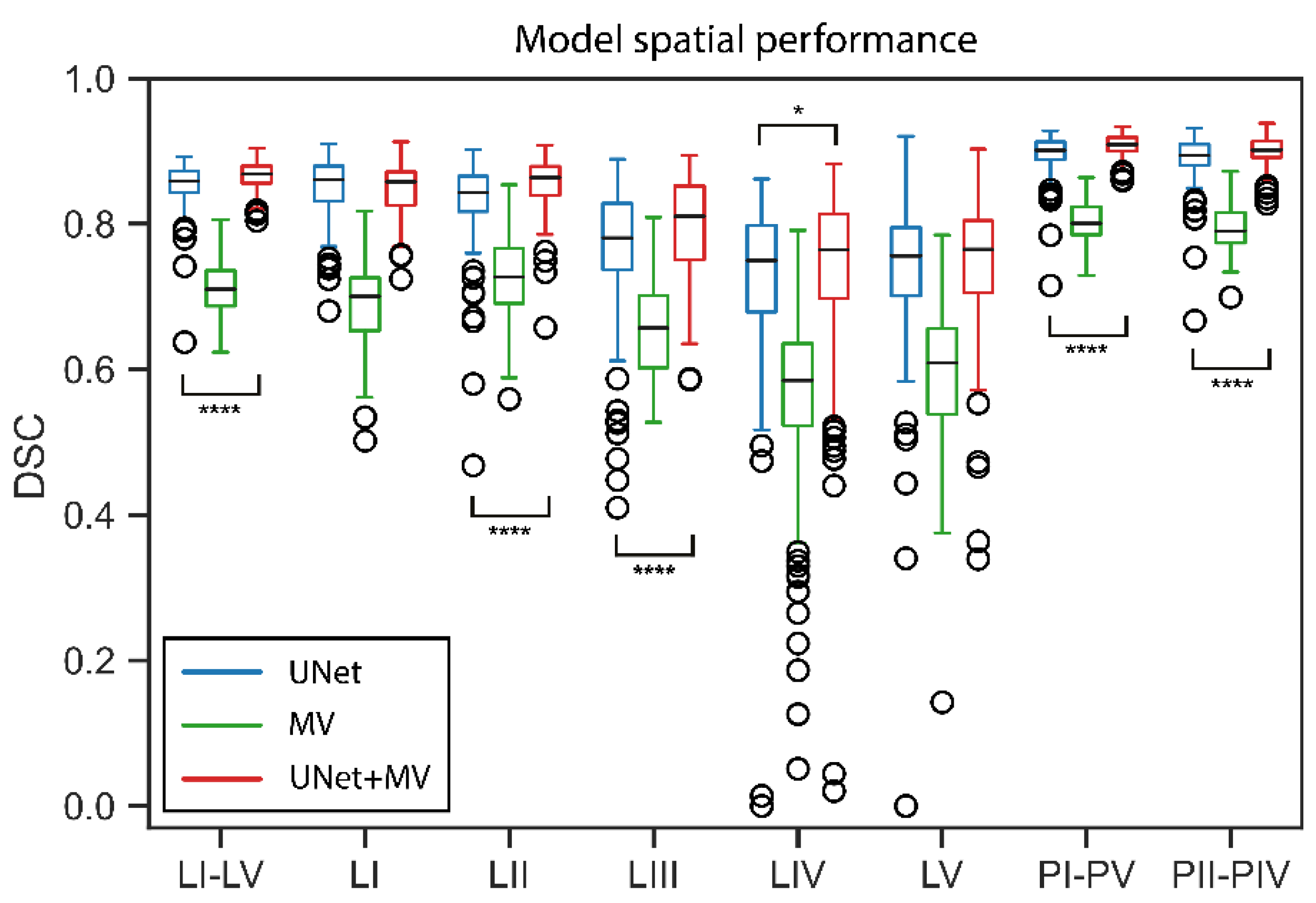
| LN I–V | [0.850–0.852] | 0.857 | [0.692–0.706] | 0.708 | [0.860–0.862] | 0.867 | 0.846 | 0.865 |
| LN I | [0.849–0.855] | 0.860 | [0.682–0.695] | 0.700 | [0.851–0.856] | 0.857 | 0.856 | 0.852 |
| LN II | [0.827–0.834] | 0.840 | [0.702–0.720] | 0.726 | [0.856–0.858] | 0.862 | 0.824 | 0.850 |
| LN III | [0.771–0.781] | 0.781 | [0.628–0.653] | 0.656 | [0.802–0.812] | 0.810 | 0.755 | 0.825 |
| LN IV | [0.714–0.746] | 0.748 | [0.559–0.585] | 0.583 | [0.757–0.764] | 0.764 | 0.743 | 0.724 |
| LN V | [0.738–0.751] | 0.754 | [0.572–0.604] | 0.610 | [0.753–0.761] | 0.763 | 0.697 | 0.707 |
| PI–PV | [0.897–0.898] | 0.899 | [0.779–0.788] | 0.798 | [0.899–0.900] | 0.908 | 0.892 | 0.904 |
| PII–PIV | [0.887–0.891] | 0.892 | [0.768–0.782] | 0.788 | [0.899–0.900] | 0.902 | 0.893 | 0.892 |
Publisher’s Note: MDPI stays neutral with regard to jurisdictional claims in published maps and institutional affiliations. |
© 2022 by the authors. Licensee MDPI, Basel, Switzerland. This article is an open access article distributed under the terms and conditions of the Creative Commons Attribution (CC BY) license (https://creativecommons.org/licenses/by/4.0/).
Share and Cite
Strijbis, V.I.J.; Dahele, M.; Gurney-Champion, O.J.; Blom, G.J.; Vergeer, M.R.; Slotman, B.J.; Verbakel, W.F.A.R. Deep Learning for Automated Elective Lymph Node Level Segmentation for Head and Neck Cancer Radiotherapy. Cancers 2022, 14, 5501. https://doi.org/10.3390/cancers14225501
Strijbis VIJ, Dahele M, Gurney-Champion OJ, Blom GJ, Vergeer MR, Slotman BJ, Verbakel WFAR. Deep Learning for Automated Elective Lymph Node Level Segmentation for Head and Neck Cancer Radiotherapy. Cancers. 2022; 14(22):5501. https://doi.org/10.3390/cancers14225501
Chicago/Turabian StyleStrijbis, Victor I. J., Max Dahele, Oliver J. Gurney-Champion, Gerrit J. Blom, Marije R. Vergeer, Berend J. Slotman, and Wilko F. A. R. Verbakel. 2022. "Deep Learning for Automated Elective Lymph Node Level Segmentation for Head and Neck Cancer Radiotherapy" Cancers 14, no. 22: 5501. https://doi.org/10.3390/cancers14225501