
Chaotic Sparrow Search Algorithm with Deep Transfer Learning Enabled Breast Cancer Classification on Histopathological Images

 , ,
, ,  ,
,  and
and 
Abstract
:Simple Summary
Abstract
1. Introduction
2. Literature Review
3. The Proposed Model
3.1. Image Pre-Processing
3.2. MixNet-Based Feature Extractor
3.3. Image Classification Using SGRU Model
3.4. Hyperparameter Optimization
4. Performance Validation
5. Conclusions
Author Contributions
Funding
Institutional Review Board Statement
Informed Consent Statement
Data Availability Statement
Conflicts of Interest
References
- Das, A.; Nair, M.S.; Peter, S.D. Computer-aided histopathological image analysis techniques for automated nuclear atypia scoring of breast cancer: A review. J. Digit. Imaging 2020, 33, 1091–1121. [Google Scholar] [CrossRef] [PubMed]
- Krithiga, R.; Geetha, P. Breast cancer detection, segmentation and classification on histopathology images analysis: A systematic review. Arch. Comput. Methods Eng. 2021, 28, 2607–2619. [Google Scholar] [CrossRef]
- Carvalho, E.D.; Antonio Filho, O.C.; Silva, R.R.; Araujo, F.H.; Diniz, J.O.; Silva, A.C.; Paiva, A.C.; Gattass, M. Breast cancer diagnosis from histopathological images using textural features and CBIR. Artif. Intell. Med. 2020, 105, 101845. [Google Scholar] [CrossRef] [PubMed]
- Xie, J.; Liu, R.; Luttrell, J., IV; Zhang, C. Deep learning based analysis of histopathological images of breast cancer. Front. Genet. 2019, 10, 80. [Google Scholar] [CrossRef] [Green Version]
- Kaushal, C.; Bhat, S.; Koundal, D.; Singla, A. Recent trends in computer assisted diagnosis (CAD) systems for breast cancer diagnosis using histopathological images. IRBM 2019, 40, 211–227. [Google Scholar] [CrossRef]
- Yan, R.; Ren, F.; Wang, Z.; Wang, L.; Zhang, T.; Liu, Y.; Rao, X.; Zheng, C.; Zhang, F. Breast cancer histopathological image classification using a hybrid deep neural network. Methods 2020, 173, 52–60. [Google Scholar] [CrossRef]
- Mehra, R. Breast cancer histology images classification: Training from scratch or transfer learning? ICT Express 2018, 4, 247–254. [Google Scholar]
- Alkassar, S.; Jebur, B.A.; Abdullah, M.A.; Al-Khalidy, J.H.; Chambers, J.A. Going deeper: Magnification-invariant approach for breast cancer classification using histopathological images. IET Comput. Vis. 2021, 15, 151–164. [Google Scholar] [CrossRef]
- Sohail, A.; Khan, A.; Wahab, N.; Zameer, A.; Khan, S. A multi-phase deep CNN based mitosis detection framework for breast cancer histopathological images. Sci. Rep. 2021, 11, 6215. [Google Scholar] [CrossRef]
- Ahmad, N.; Asghar, S.; Gillani, S.A. Transfer learning-assisted multi-resolution breast cancer histopathological images classification. Vis. Comput. 2021, 1–20. [Google Scholar] [CrossRef]
- Rai, R.; Sisodia, D.S. Real-time data augmentation based transfer learning model for breast cancer diagnosis using histopathological images. In Advances in Biomedical Engineering and Technology; Springer: Singapore, 2021; pp. 473–488. [Google Scholar]
- Alom, M.Z.; Yakopcic, C.; Nasrin, M.; Taha, T.M.; Asari, V.K. Breast cancer classification from histopathological images with inception recurrent residual convolutional neural network. J. Digit. Imaging 2019, 32, 605–617. [Google Scholar] [CrossRef] [PubMed] [Green Version]
- Vo, D.M.; Nguyen, N.Q.; Lee, S.W. Classification of breast cancer histology images using incremental boosting convolution networks. Inf. Sci. 2019, 482, 123–138. [Google Scholar] [CrossRef]
- Wang, P.; Wang, J.; Li, Y.; Li, P.; Li, L.; Jiang, M. Automatic classification of breast cancer histopathological images based on deep feature fusion and enhanced routing. Biomed. Signal Process. Control. 2021, 65, 102341. [Google Scholar] [CrossRef]
- Hirra, I.; Ahmad, M.; Hussain, A.; Ashraf, M.U.; Saeed, I.A.; Qadri, S.F.; Alghamdi, A.M.; Alfakeeh, A.S. Breast cancer classification from histopathological images using patch-based deep learning modeling. IEEE Access 2021, 9, 24273–24287. [Google Scholar] [CrossRef]
- Demir, F. DeepBreastNet: A novel and robust approach for automated breast cancer detection from histopathological images. Biocybern. Biomed. Eng. 2021, 41, 1123–1139. [Google Scholar] [CrossRef]
- Saxena, S.; Shukla, S.; Gyanchandani, M. Breast cancer histopathology image classification using kernelized weighted extreme learning machine. Int. J. Imaging Syst. Technol. 2021, 31, 168–179. [Google Scholar] [CrossRef]
- Wang, Y.; Yan, J.; Yang, Z.; Zhao, Y.; Liu, T. Optimizing GIS partial discharge pattern recognition in the ubiquitous power internet of things context: A MixNet deep learning model. Int. J. Electr. Power Energy Syst. 2021, 125, 106484. [Google Scholar] [CrossRef]
- Al Wazrah, A.; Alhumoud, S. Sentiment Analysis Using Stacked Gated Recurrent Unit for Arabic Tweets. IEEE Access 2021, 9, 137176–137187. [Google Scholar] [CrossRef]
- Yuan, J.; Zhao, Z.; Liu, Y.; He, B.; Wang, L.; Xie, B.; Gao, Y. DMPPT control of photovoltaic microgrid based on improved sparrow search algorithm. IEEE Access 2021, 9, 16623–16629. [Google Scholar] [CrossRef]
- Spanhol, F.; Oliveira, L.S.; Petitjean, C.; Heutte, L. A Dataset for Breast Cancer Histopathological Image Classification. IEEE Trans. Biomed. Eng. (TBME) 2016, 63, 1455–1462. [Google Scholar] [CrossRef]
- Reshma, V.K.; Arya, N.; Ahmad, S.S.; Wattar, I.; Mekala, S.; Joshi, S.; Krah, D. Detection of Breast Cancer Using Histopathological Image Classification Dataset with Deep Learning Techniques. BioMed Res. Int. 2022. [Google Scholar] [CrossRef] [PubMed]


| Category | Class Names | Labels | No. of Images | Total |
|---|---|---|---|---|
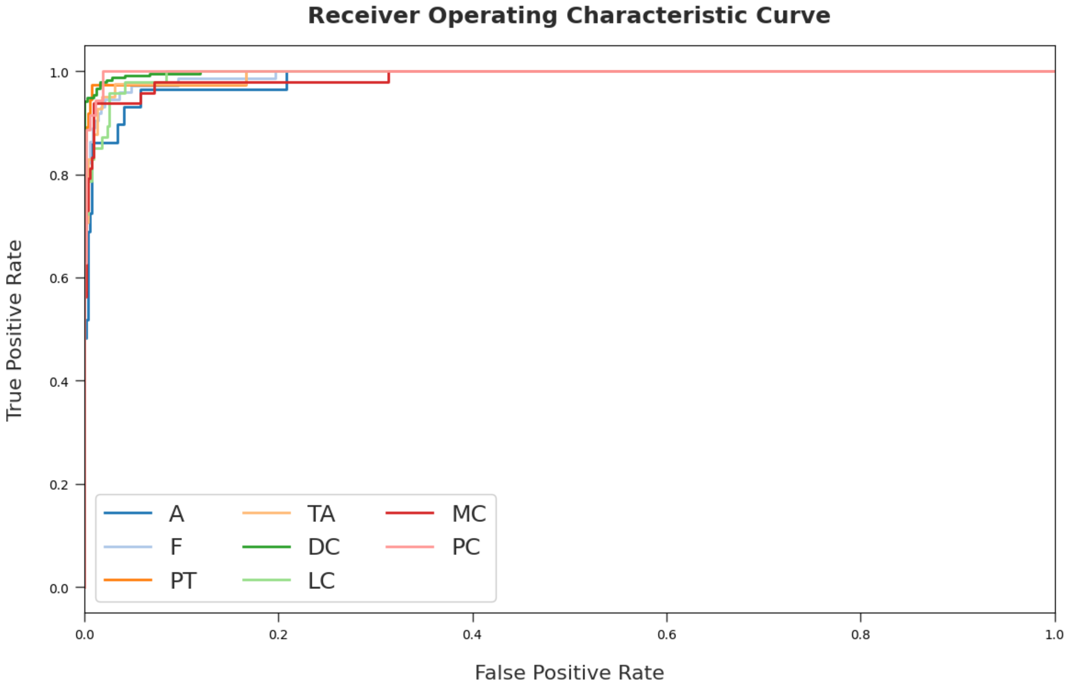
| Benign | Adenosis | A | 106 | 588 |
| Fibroadenoma | F | 237 | ||
| Phyllodes Tumor | PT | 115 | ||
| Tubular Adenoma | TA | 130 | ||
| Malignant | Carcinoma | DC | 788 | 1232 |
| Lobular Carcinoma | LC | 137 | ||
| Mucinous Carcinoma | MC | 169 | ||
| Papillary Carcinoma | PC | 138 | ||
| Total Number of Images | 1820 | |||
| Class Labels | Accuracy | Precision | Recall | Specificity | F-Score | MCC | G-Mean |
|---|---|---|---|---|---|---|---|
| Epoch-500 | |||||||
| A | 96.43 | 73.03 | 61.32 | 98.60 | 66.67 | 65.07 | 77.76 |
| F | 95.77 | 82.00 | 86.50 | 97.16 | 84.19 | 81.79 | 91.67 |
| PT | 97.25 | 83.51 | 70.43 | 99.06 | 76.42 | 75.27 | 83.53 |
| TA | 95.55 | 70.59 | 64.62 | 97.93 | 67.47 | 65.16 | 79.55 |
| DC | 92.42 | 87.36 | 96.45 | 89.34 | 91.68 | 85.10 | 92.83 |
| LC | 96.21 | 78.81 | 67.88 | 98.51 | 72.94 | 71.14 | 81.78 |
| MC | 94.84 | 73.58 | 69.23 | 97.46 | 71.34 | 68.54 | 82.14 |
| PC | 96.48 | 81.36 | 69.57 | 98.69 | 75.00 | 73.38 | 82.86 |
| Average | 95.62 | 78.78 | 73.25 | 97.09 | 75.71 | 73.18 | 84.01 |
| Epoch-1000 | |||||||
| A | 97.25 | 80.43 | 69.81 | 98.95 | 74.75 | 73.51 | 83.11 |
| F | 97.20 | 87.50 | 91.56 | 98.04 | 89.48 | 87.90 | 94.75 |
| PT | 98.13 | 89.32 | 80.00 | 99.35 | 84.40 | 83.56 | 89.15 |
| TA | 96.76 | 77.52 | 76.92 | 98.28 | 77.22 | 75.48 | 86.95 |
| DC | 95.82 | 93.20 | 97.46 | 94.57 | 95.29 | 91.61 | 96.01 |
| LC | 97.14 | 84.55 | 75.91 | 98.87 | 80.00 | 78.60 | 86.63 |
| MC | 96.98 | 83.14 | 84.62 | 98.24 | 83.87 | 82.21 | 91.18 |
| PC | 97.53 | 86.05 | 80.43 | 98.93 | 83.15 | 81.87 | 89.20 |
| Average | 97.10 | 85.21 | 82.09 | 98.16 | 83.52 | 81.84 | 89.62 |
| Epoch-1500 | |||||||
| A | 98.46 | 89.80 | 83.02 | 99.42 | 86.27 | 85.53 | 90.85 |
| F | 98.68 | 94.19 | 95.78 | 99.12 | 94.98 | 94.22 | 97.43 |
| PT | 99.23 | 93.91 | 93.91 | 99.59 | 93.91 | 93.50 | 96.71 |
| TA | 98.41 | 90.40 | 86.92 | 99.29 | 88.63 | 87.79 | 92.90 |
| DC | 98.13 | 97.12 | 98.60 | 97.77 | 97.86 | 96.21 | 98.19 |
| LC | 98.68 | 93.80 | 88.32 | 99.52 | 90.98 | 90.31 | 93.76 |
| MC | 98.52 | 89.89 | 94.67 | 98.91 | 92.22 | 91.44 | 96.77 |
| PC | 98.79 | 93.28 | 90.58 | 99.46 | 91.91 | 91.27 | 94.92 |
| Average | 98.61 | 92.80 | 91.48 | 99.14 | 92.10 | 91.29 | 95.19 |
| Epoch-2000 | |||||||
| A | 98.57 | 90.82 | 83.96 | 99.47 | 87.25 | 86.57 | 91.39 |
| F | 98.68 | 93.83 | 96.20 | 99.05 | 95.00 | 94.25 | 97.62 |
| PT | 99.18 | 92.37 | 94.78 | 99.47 | 93.56 | 93.13 | 97.10 |
| TA | 98.30 | 89.60 | 86.15 | 99.23 | 87.84 | 86.95 | 92.46 |
| DC | 98.02 | 96.65 | 98.86 | 97.38 | 97.74 | 96.00 | 98.12 |
| LC | 98.46 | 94.31 | 84.67 | 99.58 | 89.23 | 88.55 | 91.83 |
| MC | 98.68 | 91.43 | 94.67 | 99.09 | 93.02 | 92.31 | 96.86 |
| PC | 98.46 | 91.67 | 87.68 | 99.35 | 89.63 | 88.82 | 93.33 |
| Average | 98.54 | 92.58 | 90.87 | 99.08 | 91.66 | 90.82 | 94.84 |
| Methods | Accuracy | Precision | Recall | F-Score |
|---|---|---|---|---|
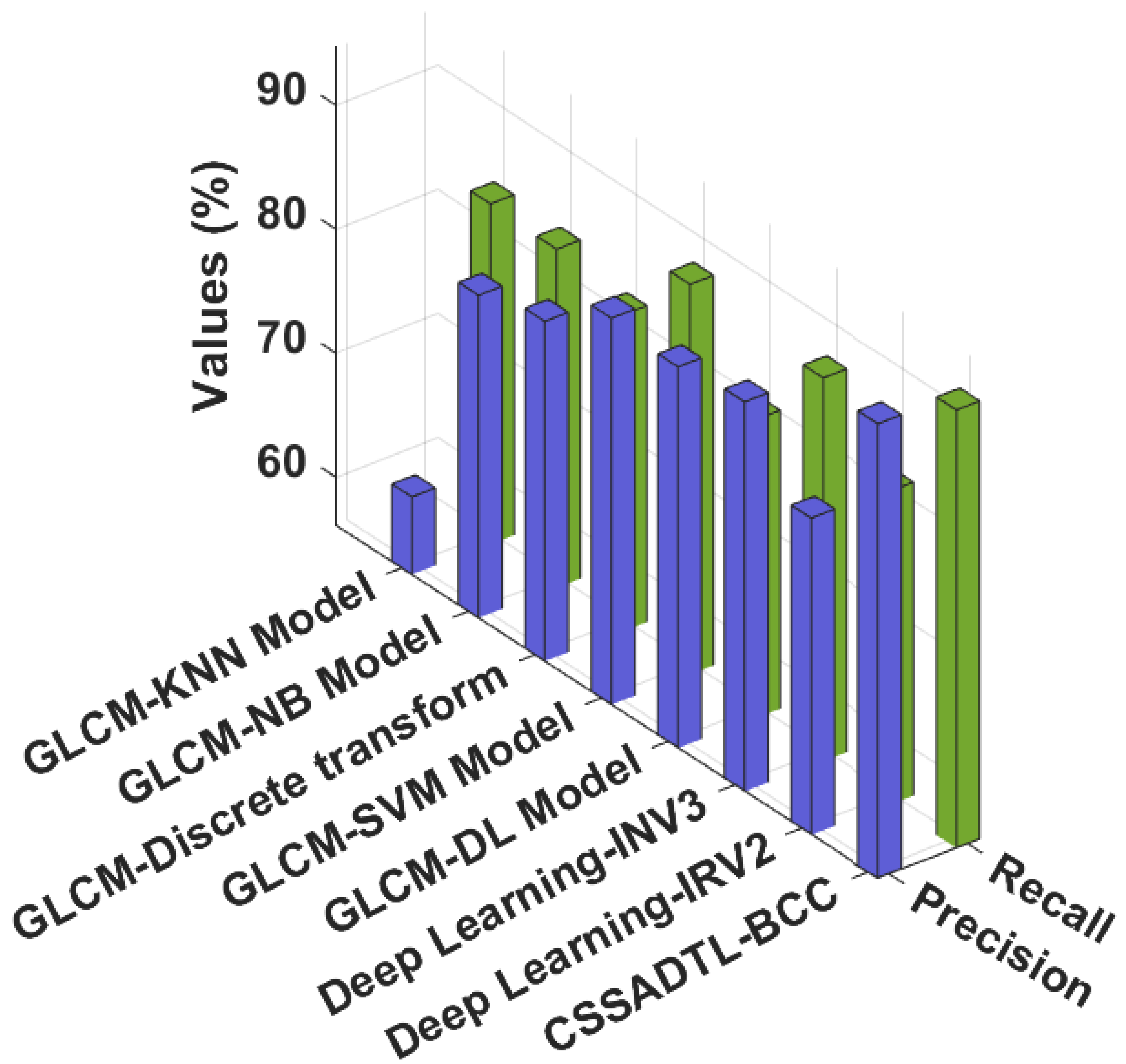
| GLCM-KNN Model | 76.17 | 62.40 | 83.60 | 82.22 |
| GLCM-NB Model | 78.45 | 82.16 | 83.45 | 86.97 |
| GLCM-Discrete transform | 85.00 | 83.56 | 81.66 | 84.69 |
| GLCM-SVM Model | 85.00 | 87.32 | 87.61 | 81.62 |
| GLCM-DL Model | 92.44 | 86.89 | 80.24 | 87.92 |
| Deep Learning-INV3 | 94.71 | 87.57 | 87.07 | 81.86 |
| Deep Learning-IRV2 | 88.12 | 81.70 | 81.44 | 86.42 |
| CSSADTL-BCC | 98.61 | 92.80 | 91.48 | 92.10 |
Publisher’s Note: MDPI stays neutral with regard to jurisdictional claims in published maps and institutional affiliations. |
© 2022 by the authors. Licensee MDPI, Basel, Switzerland. This article is an open access article distributed under the terms and conditions of the Creative Commons Attribution (CC BY) license (https://creativecommons.org/licenses/by/4.0/).
Share and Cite
Shankar, K.; Dutta, A.K.; Kumar, S.; Joshi, G.P.; Doo, I.C. Chaotic Sparrow Search Algorithm with Deep Transfer Learning Enabled Breast Cancer Classification on Histopathological Images. Cancers 2022, 14, 2770. https://doi.org/10.3390/cancers14112770
Shankar K, Dutta AK, Kumar S, Joshi GP, Doo IC. Chaotic Sparrow Search Algorithm with Deep Transfer Learning Enabled Breast Cancer Classification on Histopathological Images. Cancers. 2022; 14(11):2770. https://doi.org/10.3390/cancers14112770
Chicago/Turabian StyleShankar, K., Ashit Kumar Dutta, Sachin Kumar, Gyanendra Prasad Joshi, and Ill Chul Doo. 2022. "Chaotic Sparrow Search Algorithm with Deep Transfer Learning Enabled Breast Cancer Classification on Histopathological Images" Cancers 14, no. 11: 2770. https://doi.org/10.3390/cancers14112770