
Precision Motion Control of a Piezoelectric Actuator via a Modified Preisach Hysteresis Model and Two-Degree-of-Freedom H-Infinity Robust Control


Abstract
:1. Introduction
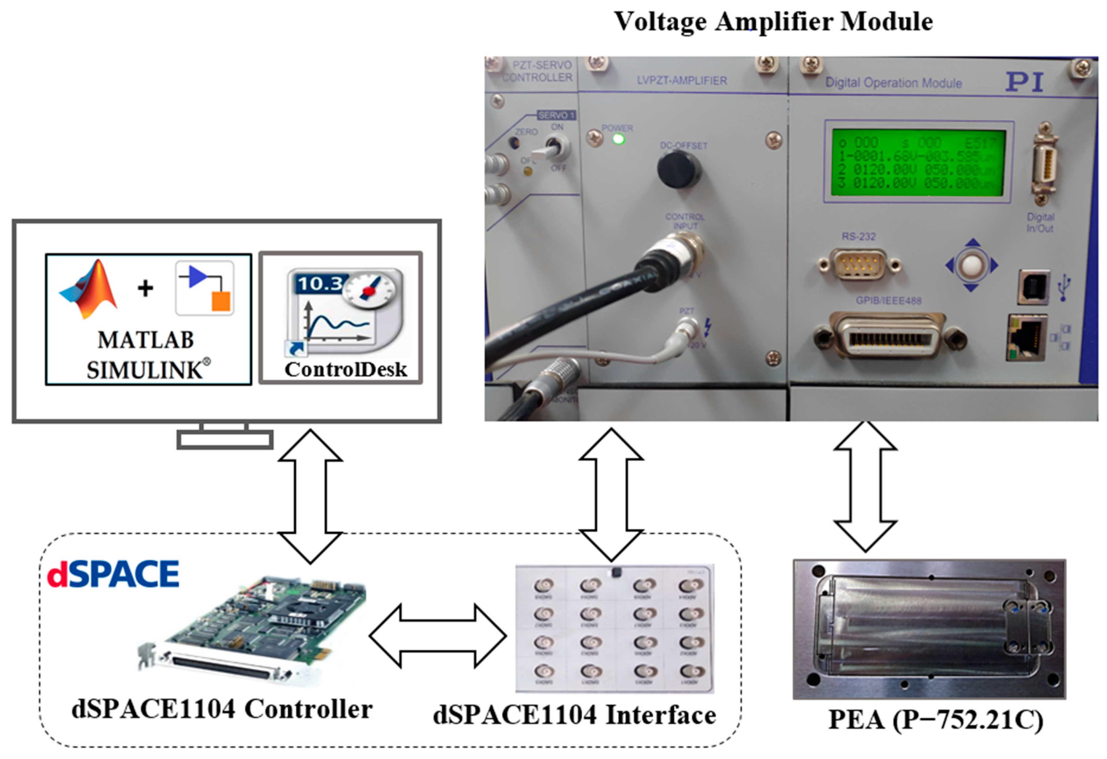
2. Experimental Setup
3. Modeling and System Identification
3.1. Linear Dynamic Model
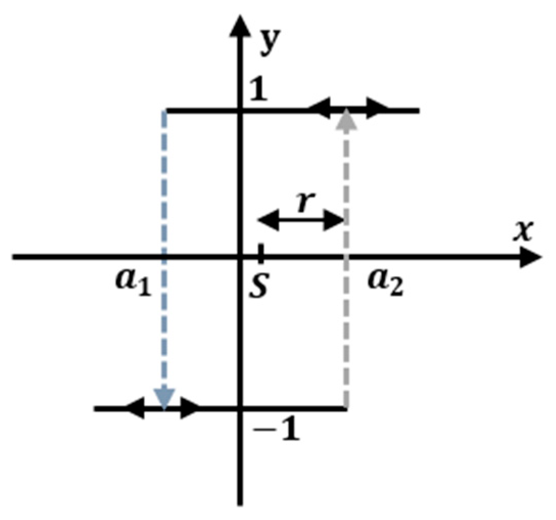
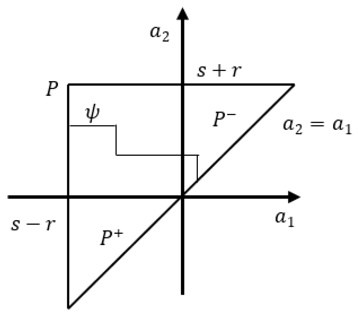
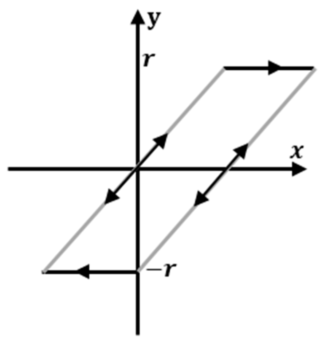
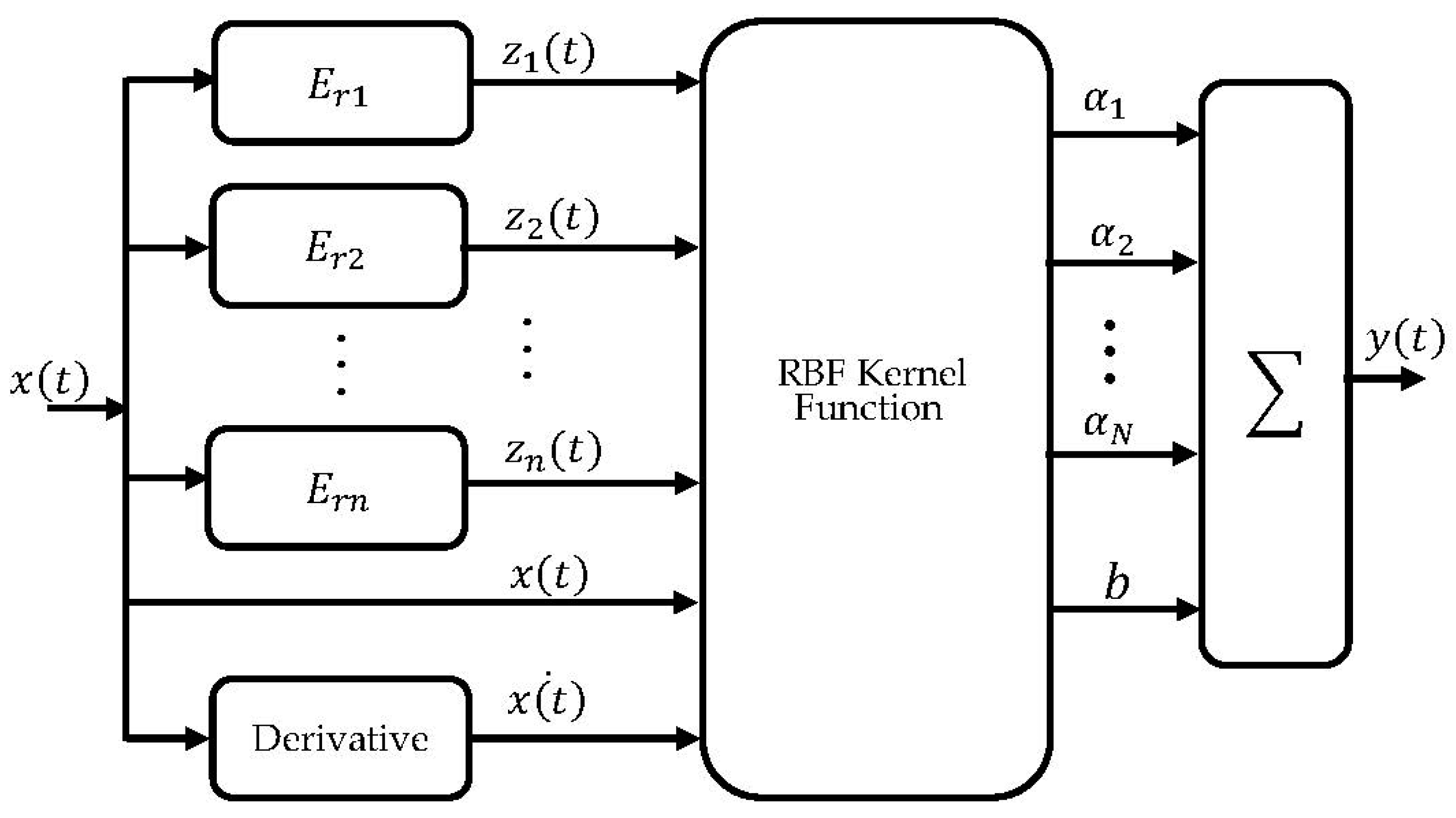
3.2. Hysteresis Modeling Using a Modified Preisach Model
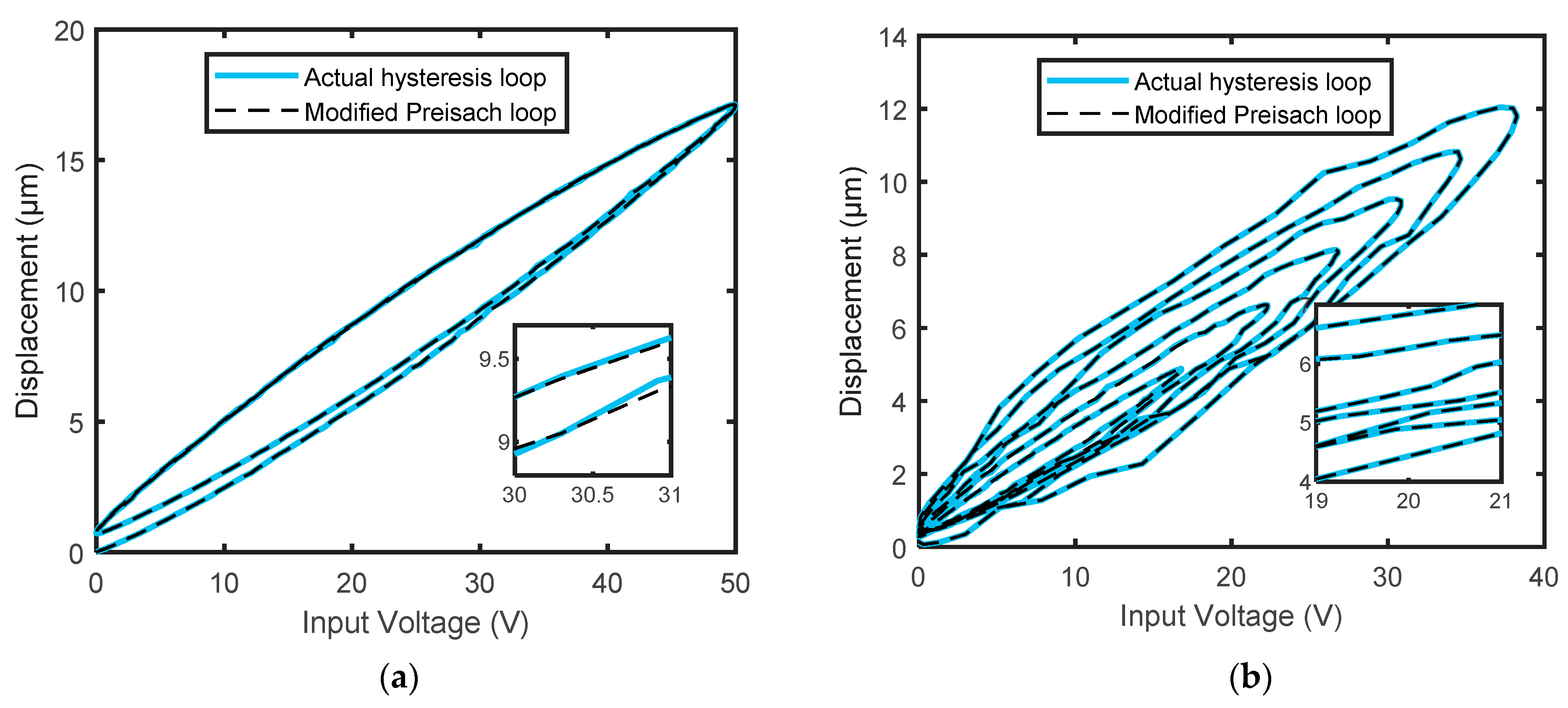
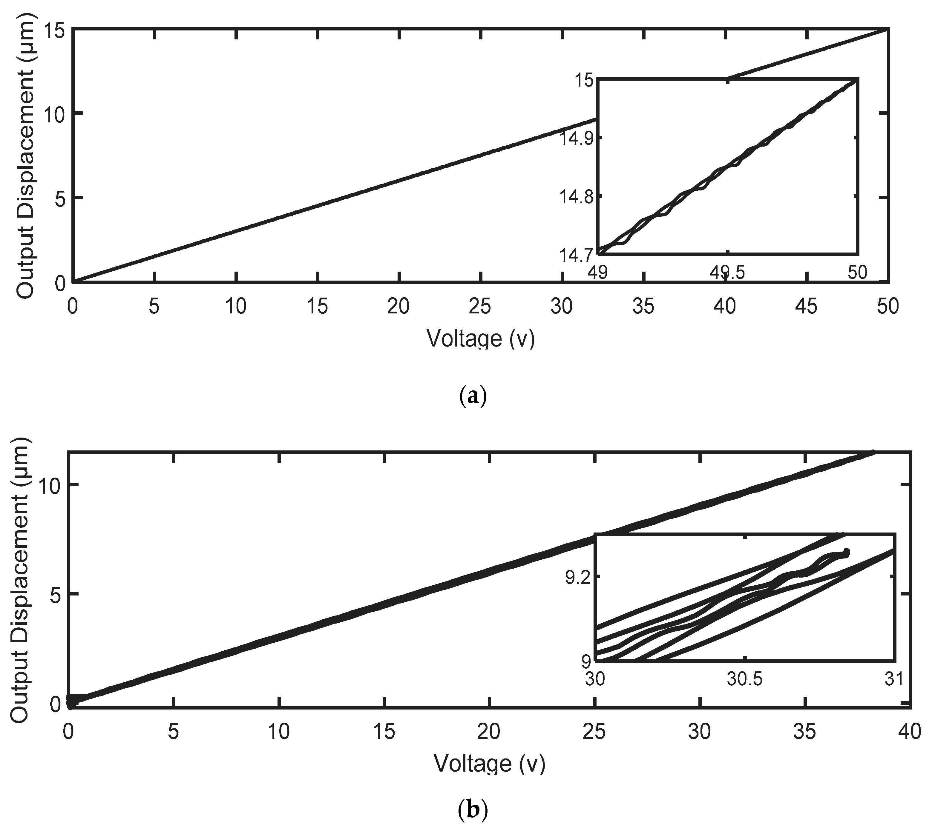
3.3. Hysteresis Modeling Results
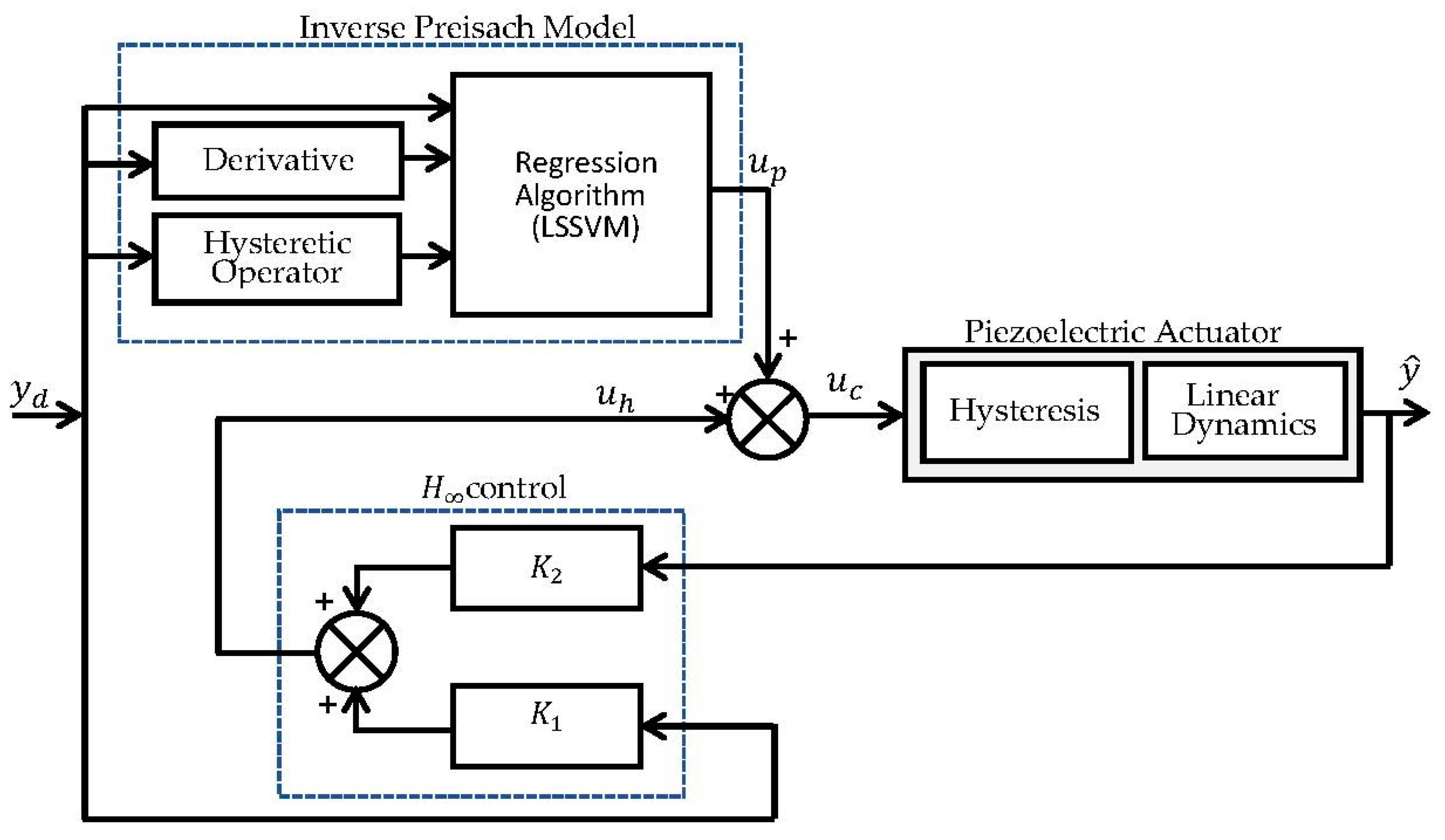
4. Hysteresis Compensation
4.1. Feedforward–Feedback Control Structure
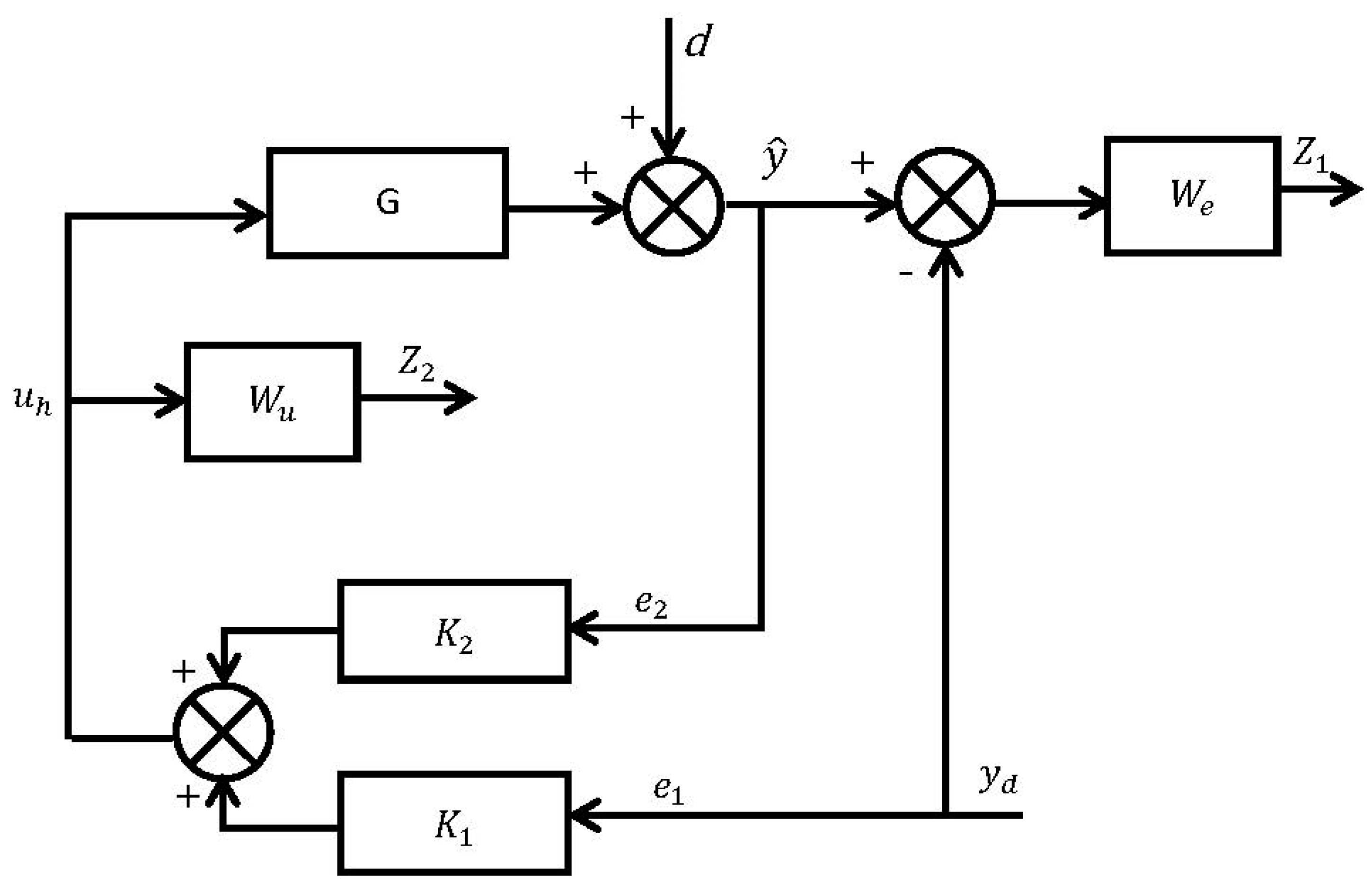
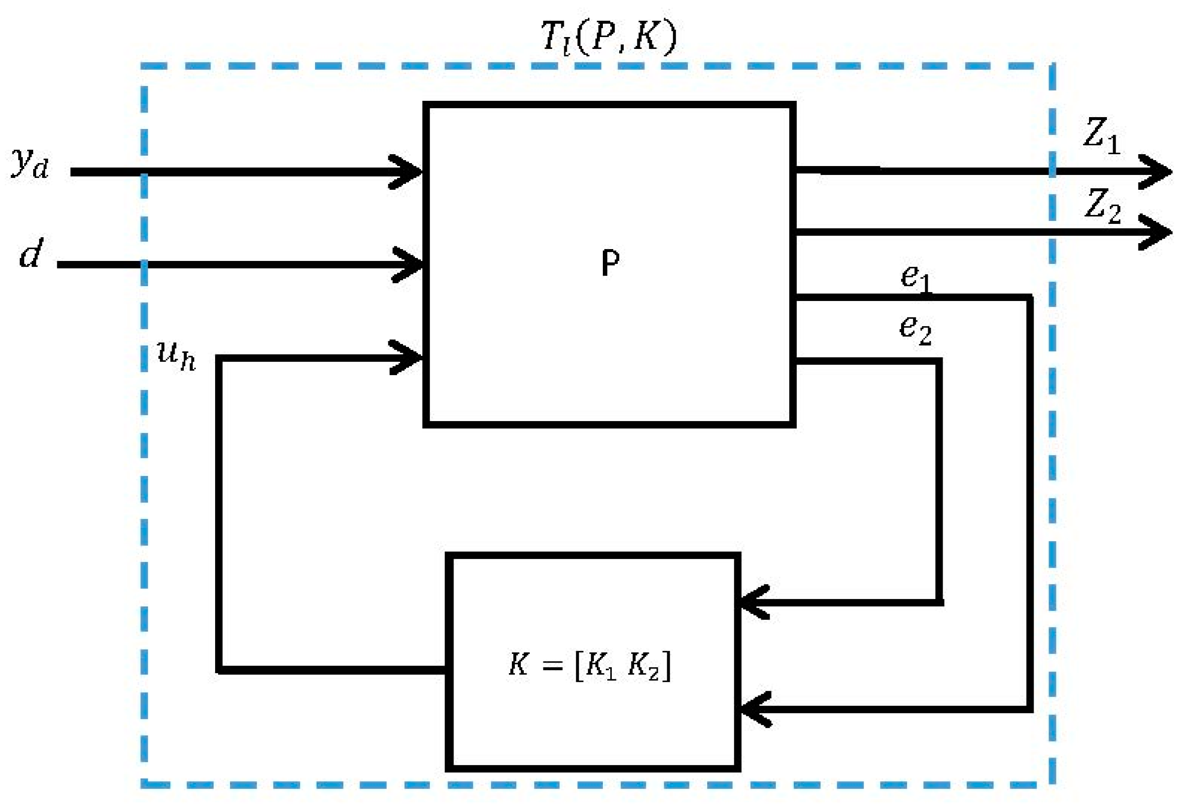
4.2. Two-Degree-of-Freedom (2-DOF) H-Infinity Controller Design
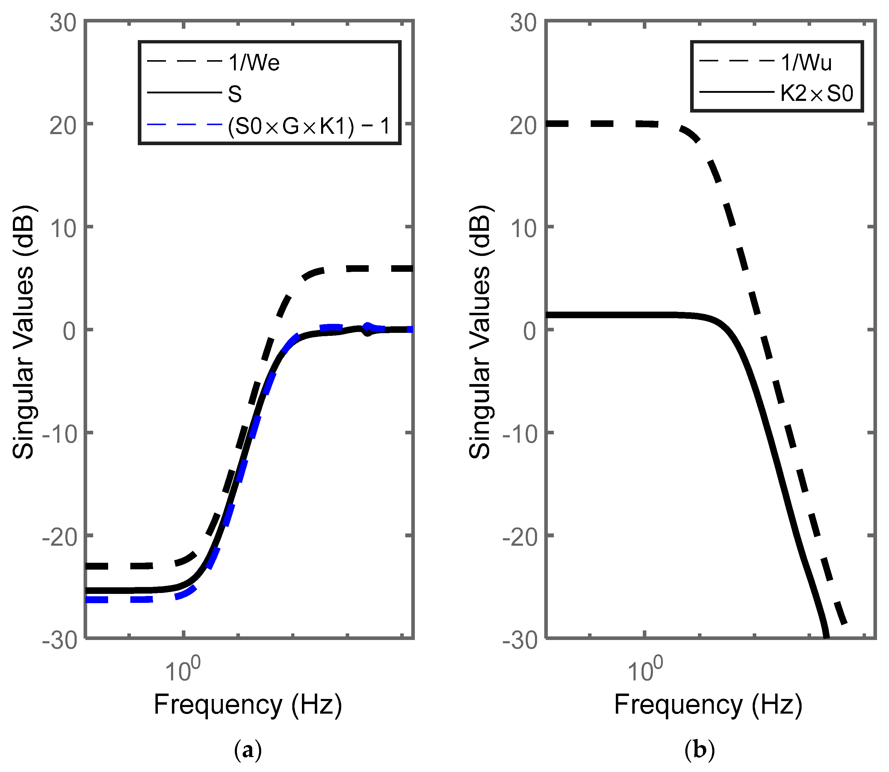
4.3. Performance Specifications and Robustness Analysis
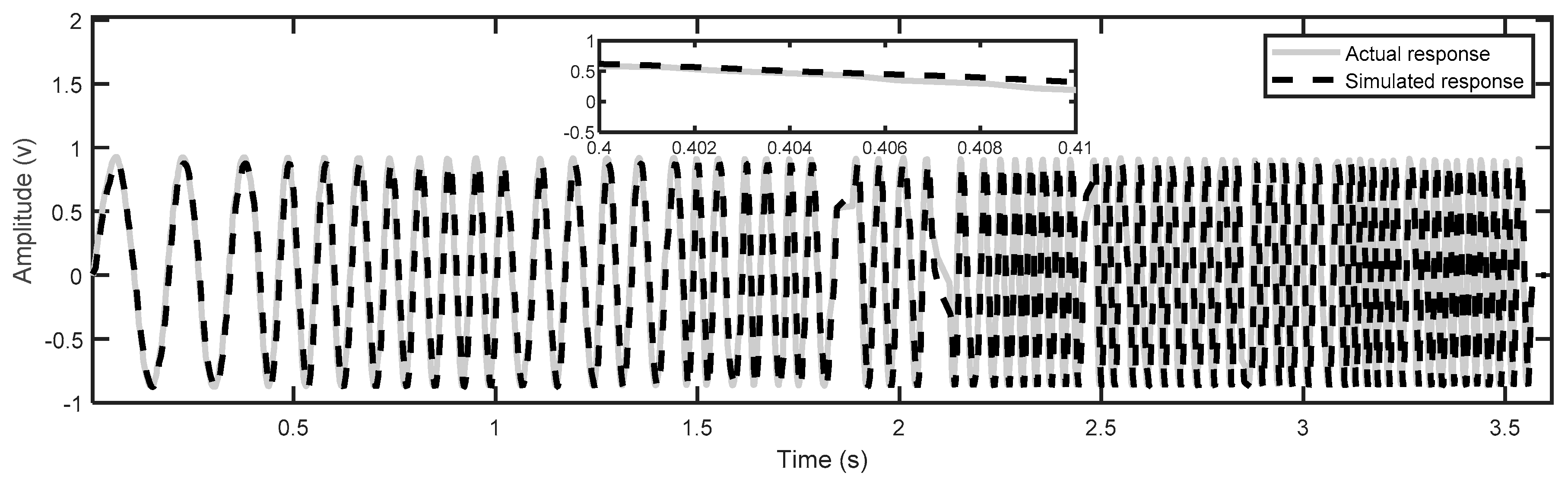
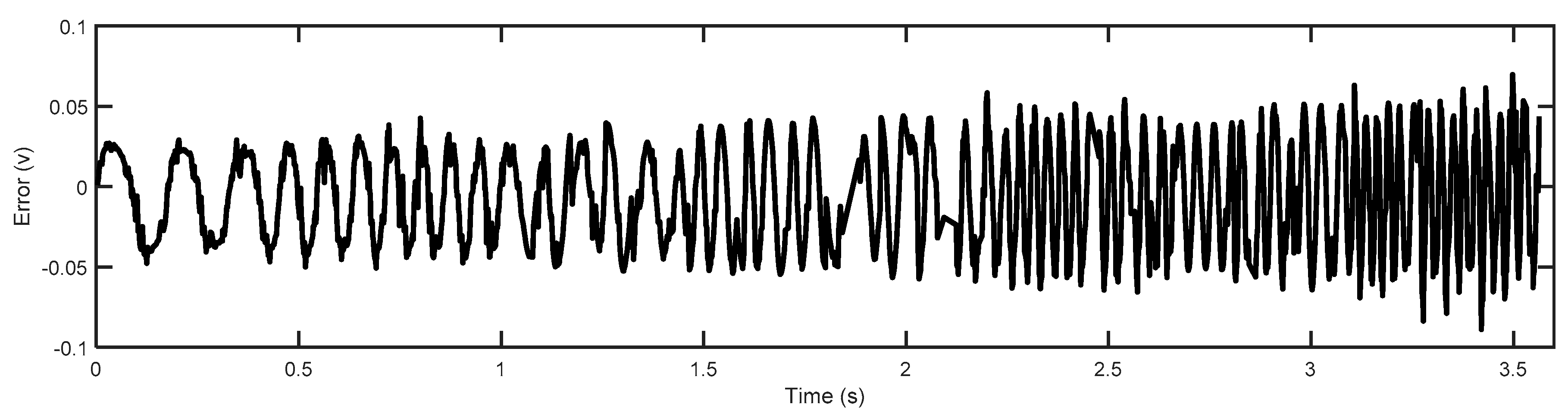
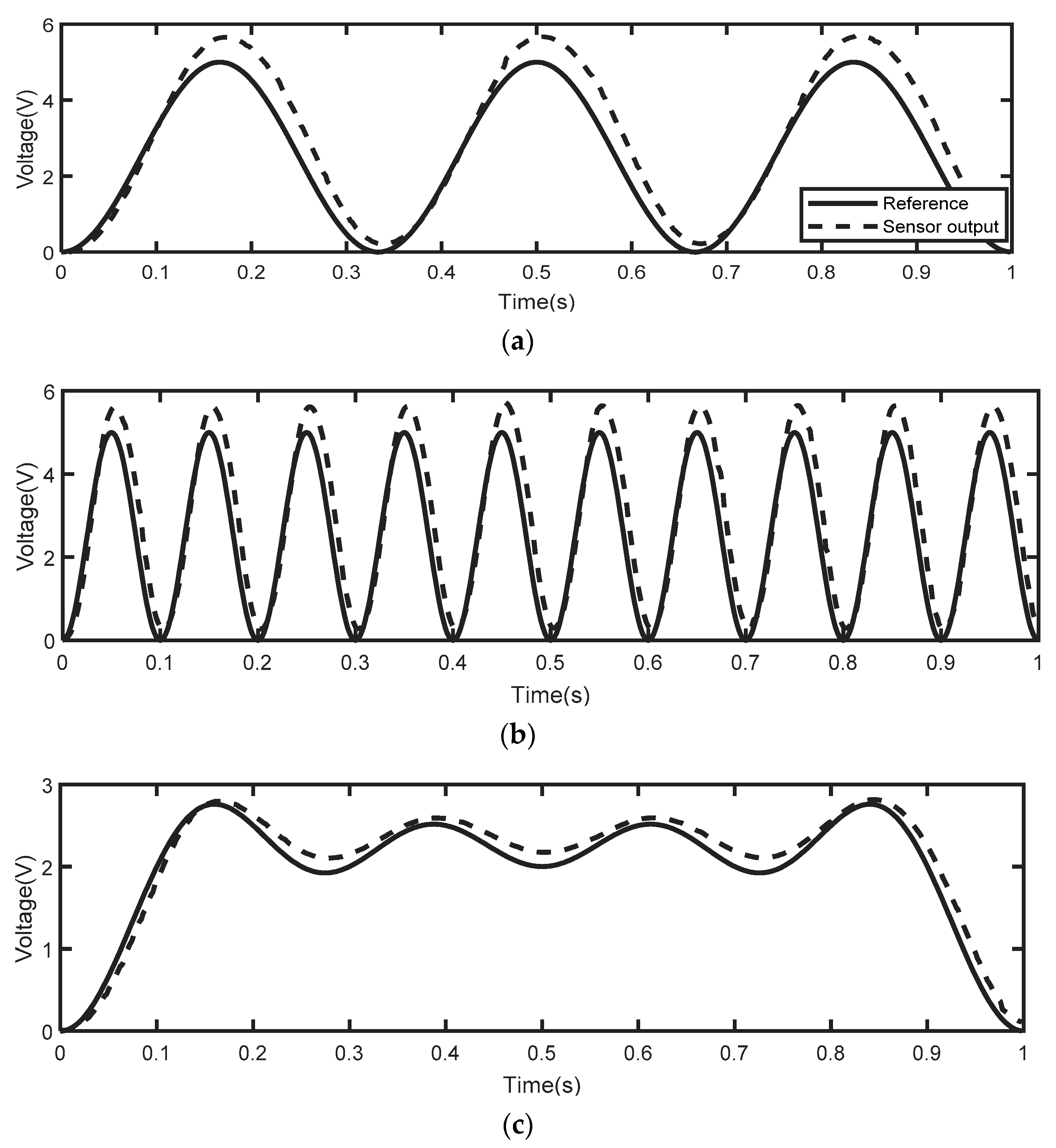
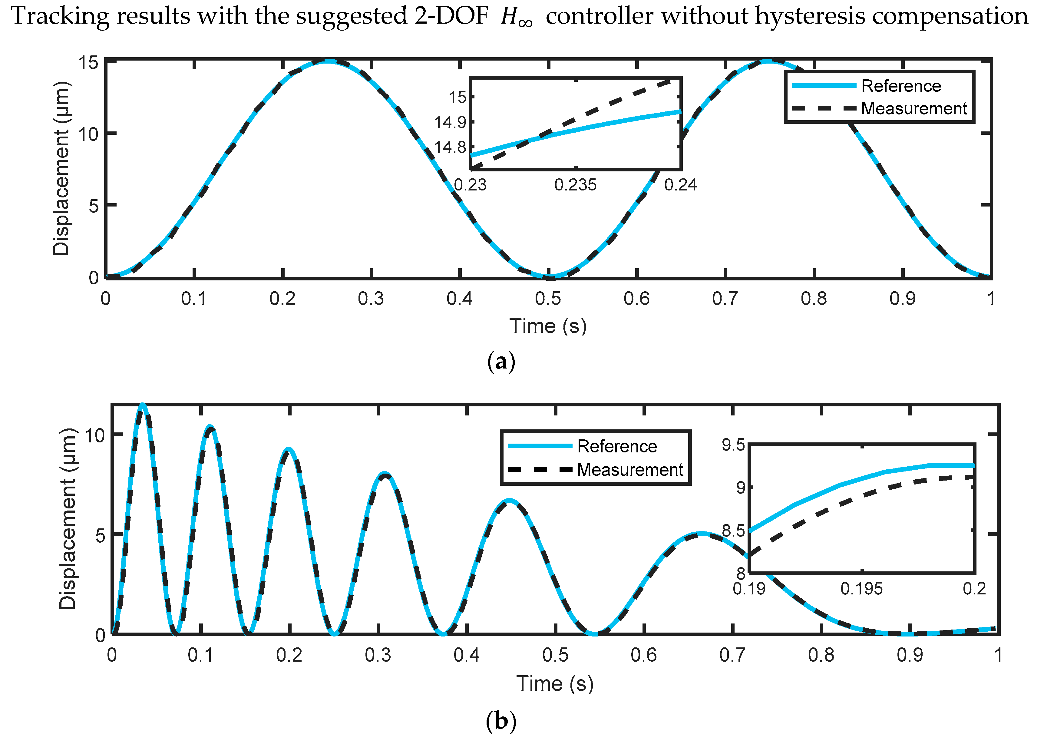
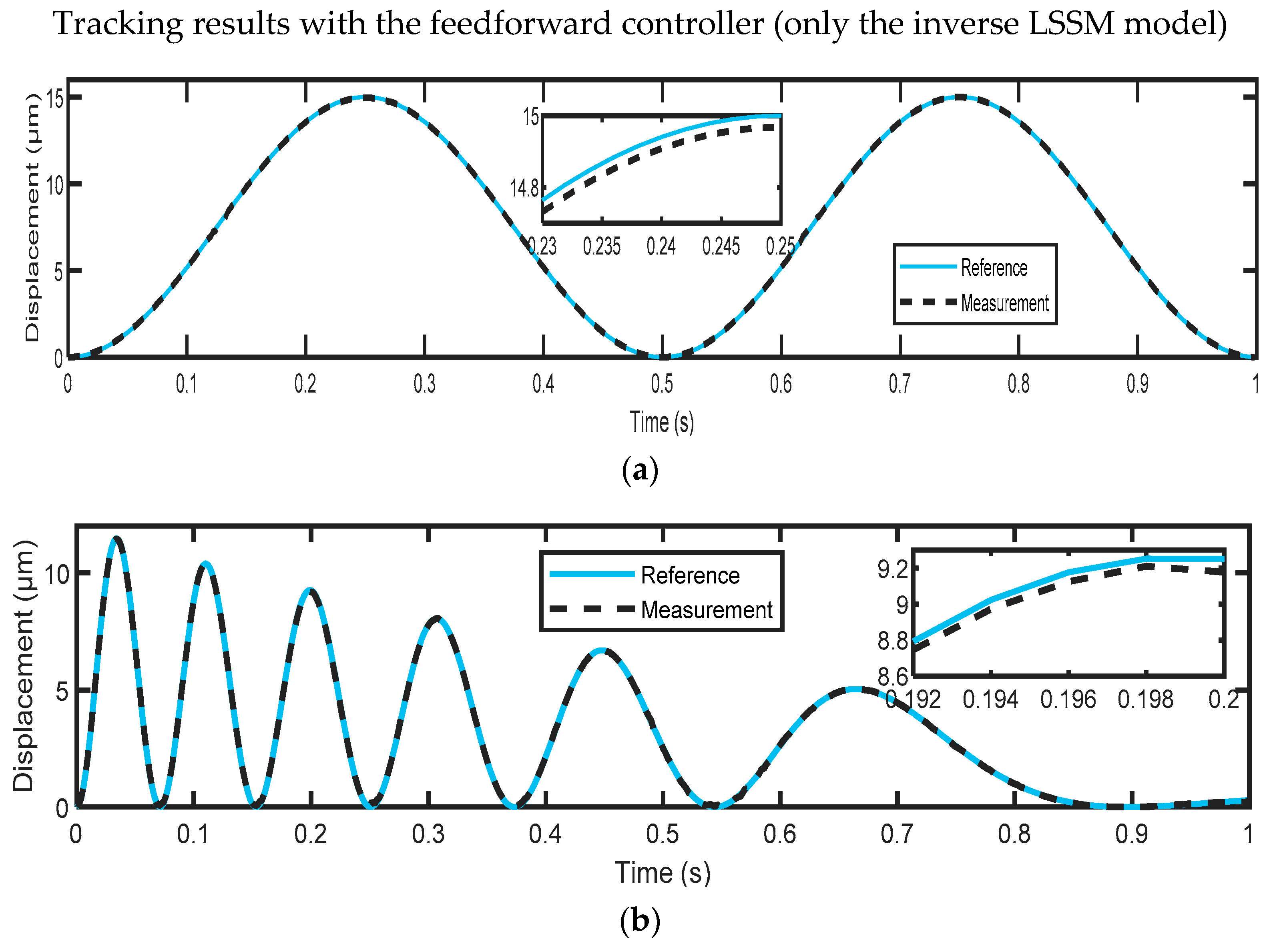
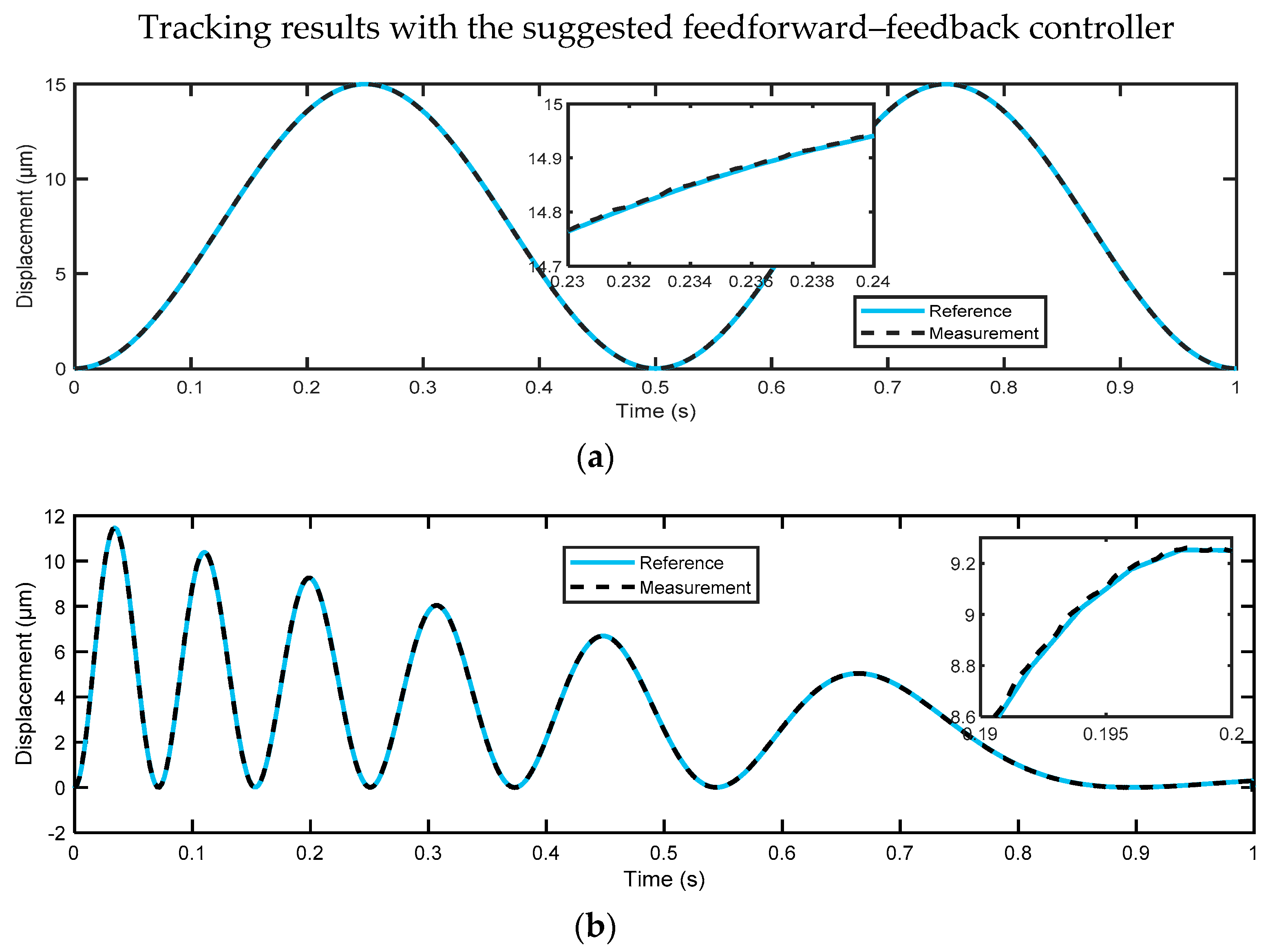
5. Tracking Results
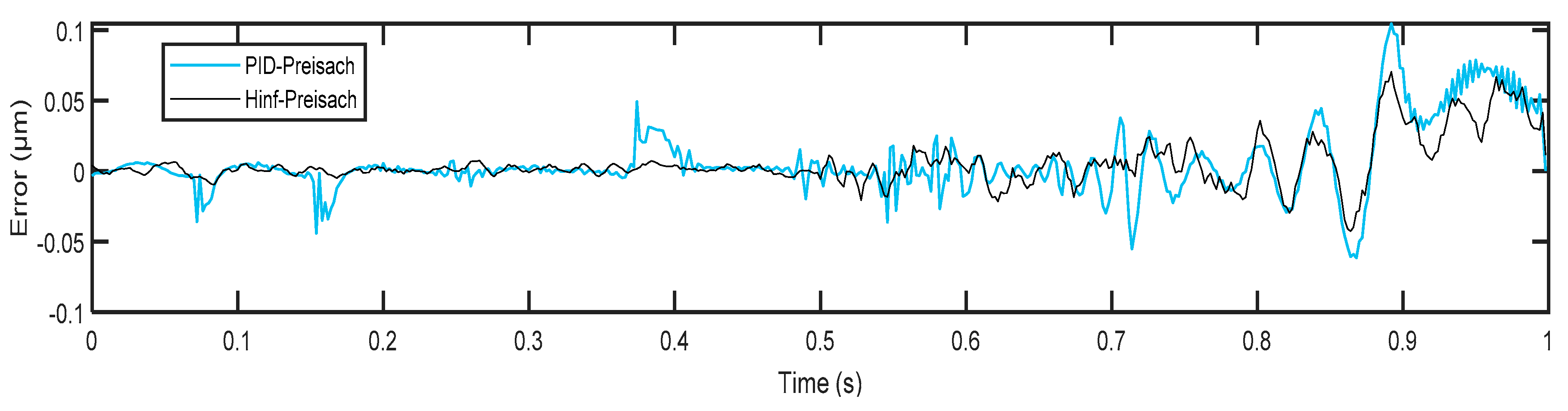
6. Comparison with Other Relevant Works
7. Conclusions
Author Contributions
Funding
Data Availability Statement
Conflicts of Interest
References
- Ji, H.-W.; Lv, B.; Wang, Y.-J.; Yang, F.; Qi, A.-Q.; Wu, X.; Ni, J. Modeling and control of rate-dependent hysteresis characteristics of piezoelectric actuators based on analog filters. Ferroelectrics 2023, 603, 94–115. [Google Scholar] [CrossRef]
- Arockiarajan, A.; Menzel, A.; Delibas, B.; Seemann, W. Computational modeling of rate0dependent domain switching in piezoelectric materials. Eur. J. Mech.—A/Solids 2006, 25, 950–964. [Google Scholar] [CrossRef] [Green Version]
- Ewing, J.A.X. Experimental researches in magnetism. Philos. Trans. R. Soc. Lond. 1885, 176, 523–640. [Google Scholar]
- Ang, W.T.; Garmón, F.A.; Khosla, P.K.; Riviere, C.N. Modeling rate-dependent hysteresis in piezoelectric actuators. In Proceedings of the 2003 IEEE/RSJ International Conference on Intelligent Robots and Systems (IROS 2003), Las Vegas, NV, USA, 27–31 October 2003; Volume 4, pp. 1975–1980. [Google Scholar]
- Janta, J. The influence of the shape of domains on the ferroelectric hysteresis loop. Ferroelectrics 1971, 1, 299–302. [Google Scholar] [CrossRef]
- Abeyaratne, R.; Kim, S.-J. Cyclic effects in shape-memory alloys: A one-dimensional continuum model. Int. J. Solids Struct. 1997, 34, 3273–3328. [Google Scholar] [CrossRef]
- Kamlah, M.; Böhle, U. Finite element analysis of piezoceramic components taking into account ferroelectric hysteresis behavior. Int. J. Solids Struct. 2001, 38, 605–633. [Google Scholar] [CrossRef]
- Al Janaideh, M.; Rakheja, S.; Su, C.-Y. Experimental characterization and modeling of rate-dependent hysteresis of a piezoceramic actuator. Mechatronics 2009, 19, 656–670. [Google Scholar] [CrossRef]
- Hu, H.; Mrad, R.B. On the classical Preisach model for hysteresis in piezoceramic actuators. Mechatronics 2003, 13, 85–94. [Google Scholar] [CrossRef]
- Ji, H.; Lv, B.; Ding, H.; Yang, F.; Qi, A.; Wu, X.; Ni, J. Modeling and Control of Hysteresis Characteristics of Piezoelectric Micro-Positioning Platform Based on Duhem Model. Actuators 2022, 11, 122. [Google Scholar] [CrossRef]
- Xu, Q.; Li, Y. Dahl model-based hysteresis compensation and precise positioning control of an XY parallel micromanipulator with piezoelectric actuation. J. Dyn. Syst. Meas. Control 2010, 4, 132. [Google Scholar] [CrossRef]
- Zhao, X.; Tan, Y. Neural network based identification of Preisach-type hysteresis in piezoelectric actuator using hysteretic operator. Sens. Actuators A Phys. 2006, 126, 306–311. [Google Scholar] [CrossRef]
- Yang, L.; Ding, B.; Liao, W.; Li, Y. Identification of preisach model parameters based on an improved particle swarm optimization method for piezoelectric actuators in micro-manufacturing stages. Micromachines 2022, 13, 698. [Google Scholar] [CrossRef] [PubMed]
- Al Janaideh, M.; Krejčí, P. Inverse rate-dependent Prandtl–Ishlinskii model for feedforward compensation of hysteresis in a piezomicropositioning actuator. IEEE ASME Trans. Mechatron. 2012, 18, 1498–1507. [Google Scholar] [CrossRef]
- Tan, U.-X.; Win, T.; Ang, W.T. Modeling piezoelectric actuator hysteresis with singularity free Prandtl-Ishlinskii model. In Proceedings of the 2006 IEEE International Conference on Robotics and Biomimetics, Kunming, China, 17–20 December 2006; pp. 251–256. [Google Scholar]
- Yang, Y.; Huang, L.; Wang, J.; Xu, Z. Expression, characterization and mutagenesis of an FAD-dependent glucose dehydro genase from Aspergillus terreus. Enzym. Microb. Technol. 2015, 68, 43–49. [Google Scholar] [CrossRef]
- Zhu, W.; Bian, L.X.; Cheng, l.; Rui, X. Non-linear compensation and displacement control of the bias-rate-dependent hysteresis of a magnetostrictive actuator. Precis. Eng. 2017, 50, 107. [Google Scholar] [CrossRef]
- Pednekar, P.; Deng, L.; Barton, T. Experimental characterization and control of a four-way non-isolating power combiner. In Proceedings of the 2016 IEEE Topical Conference on Power Amplifiers for Wireless and Radio Applications (PAWR), Austin, TX, USA, 24–27 January 2016; pp. 8–10. [Google Scholar]
- Xiao, S.; Li, Y. Modeling and high dynamic compensating the rate-dependent hysteresis of piezoelectric actuators via a novel modified inverse preisach model. IEEE Trans. Control Syst. Technol. 2012, 21, 1549–1557. [Google Scholar] [CrossRef]
- Gan, J.; Zhang, X.; Wu, H. A generalized Prandtl-Ishlinskii model for characterizing the rate-independent and rate-dependent hysteresis of piezoelectric actuators. Rev. Sci. Instrum. 2016, 87, 035002. [Google Scholar] [CrossRef] [PubMed]
- Nelles, O. Nonlinear System Identification: From Classical Approaches to Neural Networks, Fuzzy Models, and Gaussian Processes; Springer Nature: Berlin/Heidelberg, Germany, 2020. [Google Scholar]
- Suykens, J.; De Brabanter, J.; Lukas, L.; Vandewalle, J. Least Squares Support Vector Machines; World Scientific Publishing: Singapore, 2002. [Google Scholar]
- Liu, D.; Fang, Y.; Wang, H. Intelligent rate-dependent hysteresis control compensator design with Bouc-Wen model based on RMSO for piezoelectric actuator. IEEE Access 2020, 8, 63993–64001. [Google Scholar] [CrossRef]
- Ahmed, K.; Yan, P. Modeling and identification of rate dependent hysteresis in piezoelectric actuated nano-stage: A gray box neural network based approach. IEEE Access 2021, 9, 65440–65448. [Google Scholar] [CrossRef]
- Xiong, Y.; Jia, W.; Zhang, L.; Zhao, Y.; Zheng, L. Feedforward Control of Piezoelectric Ceramic Actuators Based on PEA-RNN. Sensors 2022, 22, 5387. [Google Scholar] [CrossRef]
- Huang, L.; Hu, Y.; Zhao, Y.; Li, Y. Modeling and control of IPMC actuators based on LSSVM-NARX paradigm. Mathematics 2019, 7, 741. [Google Scholar] [CrossRef] [Green Version]
- Liu, X.; Ma, Z.; Mao, X.; Shan, J.; Wang, Y. A fast and accurate piezoelectric actuator modeling method based on truncated least squares support vector regression. Rev. Sci. Instrum. 2019, 5, 055004. [Google Scholar] [CrossRef]
- Xu, Q. Identification and compensation of piezoelectric hysteresis without modeling hysteresis inverse. IEEE Trans. Ind. Electron. 2012, 60, 3927–3937. [Google Scholar] [CrossRef]
- Mao, X.; Wang, Y.; Liu, X.; Guo, Y. A hybrid feedforward-feedback hysteresis compensator in piezoelectric actuators based on least-squares support vector machine. IEEE Trans. Ind. Electron. 2017, 65, 5704–5711. [Google Scholar] [CrossRef] [Green Version]
- Farrokh, M. Hysteresis simulation using least-squares support vector machine. J. Eng. Mech. 2018, 144, 04018084. [Google Scholar] [CrossRef]
- Baziyad, A.G.; Nouh, A.S.; Ahmad, I.; Alkuhayli, A. Application of Least-Squares Support-Vector Machine Based on Hysteresis Operators and Particle Swarm Optimization for Modeling and Control of Hysteresis in Piezoelectric Actuators. Actuators 2022, 11, 217. [Google Scholar] [CrossRef]
- Baziyad, A.G.; Ahmad, I.; Ali, A.E.A. Generalization Enhancement of Operator-LSSVM-Based Hysteresis Model Using Improved Particle Swarm Optimization for Piezoelectric Actuators. In Proceedings of the 2022 IEEE 1st Industrial Electronics Society Annual On-Line Conference (ONCON), Kharagpur, India, 9–11 December 2022; pp. 88–93. [Google Scholar]
- Ahamd, I.; Abdurraqeeb, A.M. H∞ control design with feed-forward compensator for hysteresis compensation in piezoelectric actuators. Automatika 2016, 57, 691–702. [Google Scholar] [CrossRef] [Green Version]
- Yan, X.; Wang, P.; Qing, J.; Wu, S.; Zhao, F. Robust power control design for a small pressurized water reactor using an H infinity mixed sensitivity method. Nucl. Eng. Technol. 2020, 52, 1443–1451. [Google Scholar] [CrossRef]
- Cheng, S.; Li, L.; Liu, C.-Z.; Wu, X.; Fang, S.-N.; Yong, J.-W. Robust LMI-based H-infinite controller integrating AFS and DYC of autonomous vehicles with parametric uncertainties. IEEE Trans. Syst. Man Cybern. Syst. 2020, 51, 6901–6910. [Google Scholar] [CrossRef]
- Modabbernia, M.; Alizadeh, B.; Sahab, A.; Moghaddam, M.M. Robust control of automatic voltage regulator (AVR) with real structured parametric uncertainties based on H∞ and μ-analysis. ISA Trans. 2020, 100, 46–62. [Google Scholar] [CrossRef]
- Physik Instrumente. P-752 High-Precision Nanopositioning Stage. Available online: https://www.physikinstrumente.com/en/products/nanopositioning-piezo-flexure-stages/linear-piezo-flexure-stages/p-752-high-precision-nanopositioning-stage-200800/ (accessed on 14 July 2022).
- Physik Instrumente. E-505 Piezo Amplifier Module. Available online: https://www.physikinstrumente.com/en/products/controllers-and-drivers/nanopositioning-piezo-controllers/e-505-piezo-amplifier-module-602300/ (accessed on 15 July 2022).
- dSPACE. DS1104 R&D Controller Board. Available online: https://www.dspace.com/en/inc/home/products/hw/singbord/ds1104.cfm (accessed on 14 July 2022).
- LJUNG, L.; Söderström, T. Theory and Practice of Recursive Identification; MIT Press: Cambridge, MA, USA, 1983; pp. 12–42. [Google Scholar]
- Mayergoyz, I. Mathematical models of hysteresis. IEEE Trans. Magn. 1986, 22, 603–608. [Google Scholar] [CrossRef] [Green Version]
- Brokate, M.; Sprekels, J. Hysteresis and Phase Transitions; Springer Science & Business Media: Berlin/Heidelberg, Germany, 1996; Volume 121. [Google Scholar]
- Suykens, J.A.; Vandewalle, J.; De Moor, B. Optimal control by least squares support vector machines. Neural Netw. 2001, 14, 23–35. [Google Scholar] [CrossRef]
- Gordon, G.; Tibshirani, R. Karush-kuhn-tucker conditions. Optimization 2012, 10, 725. [Google Scholar]
- Eberhart, R.C.; Shi, Y.; Kennedy, J. Swarm Intelligence; Elsevier: Amsterdam, The Netherlands, 2001; pp. 287–324. [Google Scholar]
- Kennedy, J.; Eberhart, R. Particle swarms optimization. In Proceedings of the IEEE International Conference on Neural Networks, Perth, Australia, 27 November–1 December 1995; Volume 4. [Google Scholar]
- De Brabanter, K.; Karsmakers, P.; Ojeda, F.; Alzate, C.; De Brabanter, J.; Pelckmans, K.; De Moor, B.; Vandewalle, J.; Suykens, J.A. LS-SVMlab Toolbox User’s Guide: Version 1.7; Katholieke Universiteit Leuven: Leuven, Belgium, 2010. [Google Scholar]
- Sabarianand, D.; Karthikeyan, P.; Muthuramalingam, T. A review on control strategies for compensation of hysteresis and creep on piezoelectric actuators based micro systems. Mech. Syst. Signal Process. 2020, 140, 106634. [Google Scholar] [CrossRef]
- Gu, G.-Y.; Zhu, L.-M.; Su, C.-Y.; Ding, H.; Fatikow, S. Modeling and control of piezo-actuated nanopositioning stages: A survey. IEEE Trans. Autom. Sci. Eng. 2014, 13, 313–332. [Google Scholar] [CrossRef]
- Gu, D.-W.; Petkov, P.; Konstantinov, M.M. Robust Control Design with MATLAB®; Springer Science & Business Media: Glasgow, UK, 2005; pp. 194–199. [Google Scholar]
- Boukarim, G.E.; Chow, J.H. Modeling of nonlinear system uncertainties using a linear fractional transformation approach. In Proceedings of the 1998 American Control Conference. ACC (IEEE Cat. No. 98CH36207), Philadelphia, PA, USA, 26–26 June 1998; pp. 2973–2979. [Google Scholar]
- Ang, W.T.; Khosla, P.K.; Riviere, C.N. Feedforward controller with inverse rate-dependent model for piezoelectric actuators in trajectory-tracking applications. IEEE/ASME Trans. Mechatron. 2007, 12, 134–142. [Google Scholar] [CrossRef] [Green Version]
- Badr, B.M.; Ali, W.G. Identification and control for a single-axis PZT nanopositioner stage. In Proceedings of the Fourth International Conference on Modeling, Simulation and Applied Optimization, Kuala Lumpur, Malaysia, 19–21 April 2011; pp. 1–6. [Google Scholar]
- Chen, Z.; Zheng, J.; Zhang, H.-T.; Ding, H. Tracking of piezoelectric actuators with hysteresis: A nonlinear robust output regulation approach. Int. J. Robust Nonlinear Control 2016, 27, 2610–2626. [Google Scholar] [CrossRef]
- Zheng, J.; Fu, M. High-bandwidth control design for a piezoelectric nanopositioning stage. In Proceedings of the 2011 9th IEEE International Conference on Control and Automation (ICCA), Santiago, Chile, 19–21 December 2011; 2011; pp. 760–765. [Google Scholar]


| Parameter | Value |
|---|---|
| Samples/second | 500 |
| Range of reference signal amplitudes | 0–6 V |
| Number of hysteresis operators | 55 |
| Acceleration parameters | 2 |
| Population size | 30 |
| Minimum and maximum inertia weights of particles | [0.4, 0.9] |
| Iterations | 100 |
| Hyper-parameters | C = , = 3.135 |
| Bias | 1.831 |
| Function | Description |
|---|---|
| The weighted error between the ideal and actual closed-loop system | |
| Weighted output sensitivity | |
| Weighted control action that can occur due to reference | |
| Weighted control action that can occur due to disturbance |
| Constraint | Description |
|---|---|
| For good robustness and sufficient stability margin | |
| For good disturbance attenuation and less tracking error | |
| To avoid saturation of the control signal |
| Parameter | Value | Parameter | Value |
|---|---|---|---|
| 0 | 0 | ||
| 1.315 | −1.315 | ||
| 6.880 | −6.880 | ||
| 8.559 | −8.559 | ||
| 1.544 | −1.544 | ||
| 8.003 | −8.003 | ||
| 2.927 | −2.927 | ||
| 1 | 1 | ||
| 1.477 | 1.477 | ||
| 1.652 | 1.652 | ||
| 3.515 | 3.515 | ||
| 1.948 | 1.948 | ||
| 7.649 | 7.649 | ||
| 1.339 | 1.339 |
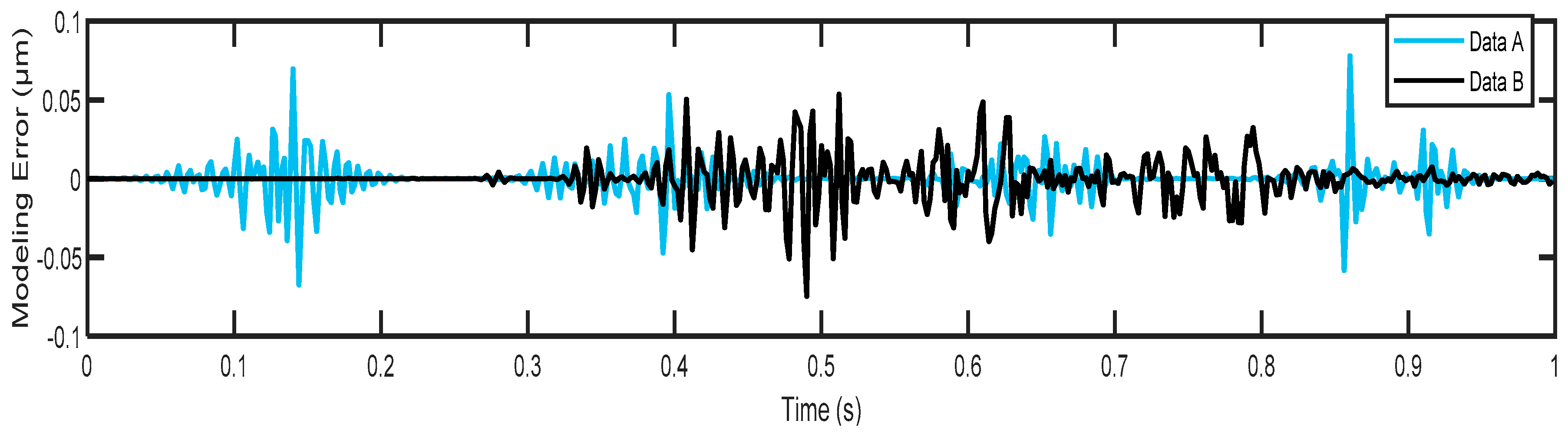
| Data | RMSE (μm) | Percentage of Improvement % | |
|---|---|---|---|
| PID-Preisach | Proposed | ||
| A | 0.0214 | 0.0190 | 11.2 |
| B | 0.0267 | 0.0233 | 12.7 |
| Mean | 0.0241 | 0.0212 | 12.03 |
| Method | Control Structure | Type of PEA | RMSE (μm) |
|---|---|---|---|
| LSSVM [28] | The feedforward–feedback controller was designed by LSSVM without modeling hysteresis. | PEA actuator (T434-A4-201, Piezo Systems, Inc., Cambridge, MA, USA) | 0.62 |
| RNN [25] | The feedforward compensator was developed by the deep learning method (RNN). | PEA actuator (P-621.1CD, Karlsruhe, Germany, PI Co.) | 0.465 |
| Modified Preisach [52] | The feedforward compensator was developed by the improved inverse Preisach. | PEA actuator (P-885.50, PI Co.) | 0.15 |
| PID-NARX-LSSVM [26] | The feedforward compensator was designed by the least-squares support vector machine and the feedback controller was designed by PID. | PEA actuator (name of the company is unavailable) | 0.03 |
| PID-Modified Preisach [31] | The feedforward compensator was designed by modified Preisach using PSO-LSSVM and the feedback controller was designed by incremental PID control. | Same actuator (P-752.21C) | 0.0241 |
| Fuzzy-PID control [53] | The FB compensator was designed by the fuzzy PI controller. | Same actuator (P-752.21C) | 0.333 |
| Modified Bouc–Wen [54] | The nonlinear internal model (estimator) coupled with the Bouc–Wen model for only rate-independent hysteresis. | Same actuator (P-752.21C) | Maximum = 0.015 (for rate-independent hysteresis) |
| CLC/MRF controller [55] | A complex lead compensator (CLC) using the phase-stabilized compensation method, combined with a multi-resonant filter (MRF). | Same actuator (P-752.21C) | 0.0278 |
| The proposed method | The feedforward compensator was designed by modified Preisach using PSO-LSSVM and the feedback controller was designed by the 2-DOF control. | (P-752.21C) | 0.0212 |
Disclaimer/Publisher’s Note: The statements, opinions and data contained in all publications are solely those of the individual author(s) and contributor(s) and not of MDPI and/or the editor(s). MDPI and/or the editor(s) disclaim responsibility for any injury to people or property resulting from any ideas, methods, instructions or products referred to in the content. |
© 2023 by the authors. Licensee MDPI, Basel, Switzerland. This article is an open access article distributed under the terms and conditions of the Creative Commons Attribution (CC BY) license (https://creativecommons.org/licenses/by/4.0/).
Share and Cite
Baziyad, A.G.; Ahmad, I.; Salamah, Y.B. Precision Motion Control of a Piezoelectric Actuator via a Modified Preisach Hysteresis Model and Two-Degree-of-Freedom H-Infinity Robust Control. Micromachines 2023, 14, 1208. https://doi.org/10.3390/mi14061208
Baziyad AG, Ahmad I, Salamah YB. Precision Motion Control of a Piezoelectric Actuator via a Modified Preisach Hysteresis Model and Two-Degree-of-Freedom H-Infinity Robust Control. Micromachines. 2023; 14(6):1208. https://doi.org/10.3390/mi14061208
Chicago/Turabian StyleBaziyad, Ayad G., Irfan Ahmad, and Yasser Bin Salamah. 2023. "Precision Motion Control of a Piezoelectric Actuator via a Modified Preisach Hysteresis Model and Two-Degree-of-Freedom H-Infinity Robust Control" Micromachines 14, no. 6: 1208. https://doi.org/10.3390/mi14061208