
Tree-Based Machine Learning Models with Optuna in Predicting Impedance Values for Circuit Analysis
 , ,
, ,
Abstract
:1. Introduction
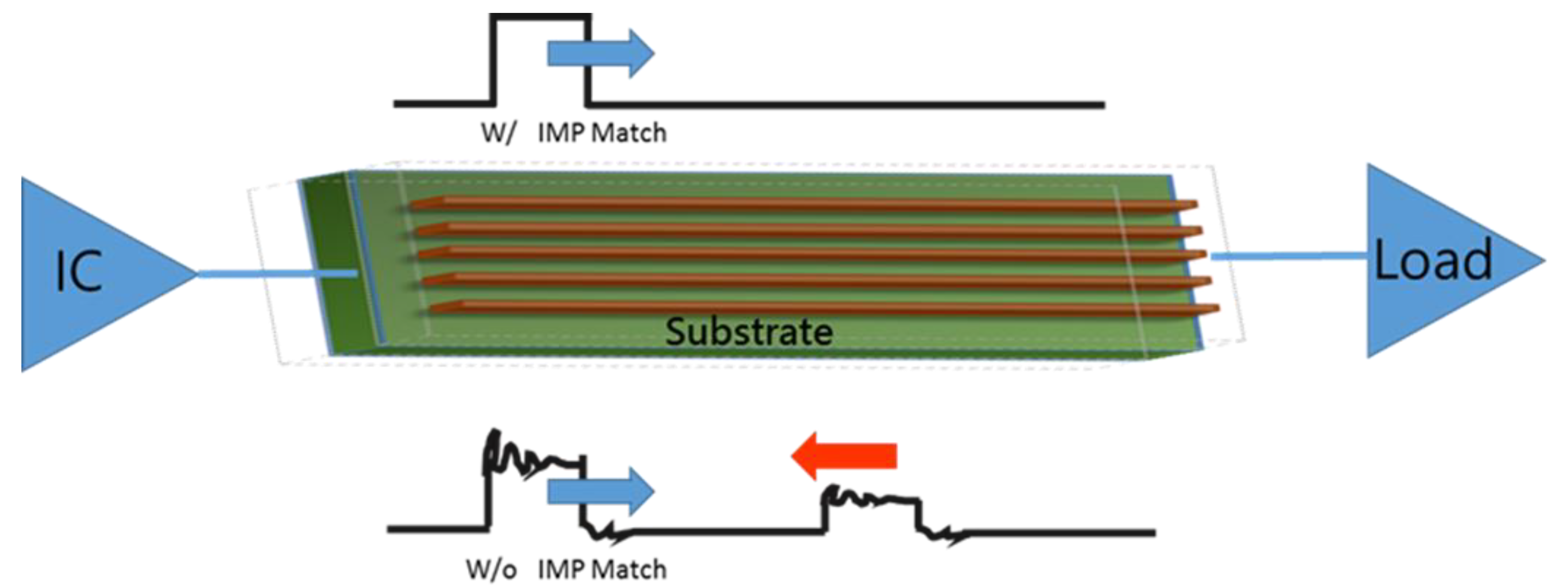
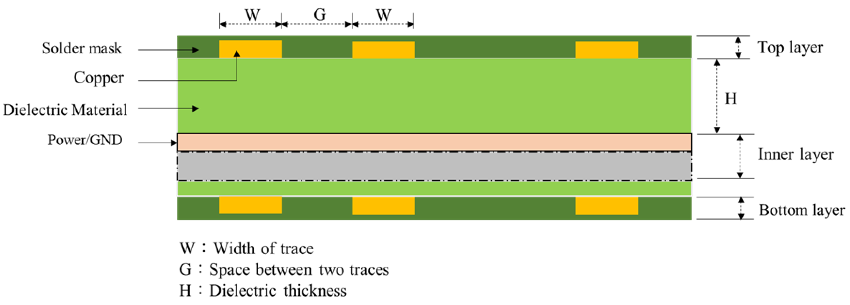
2. IC-PCB Circuit Signal Transmission and Substrate Structure
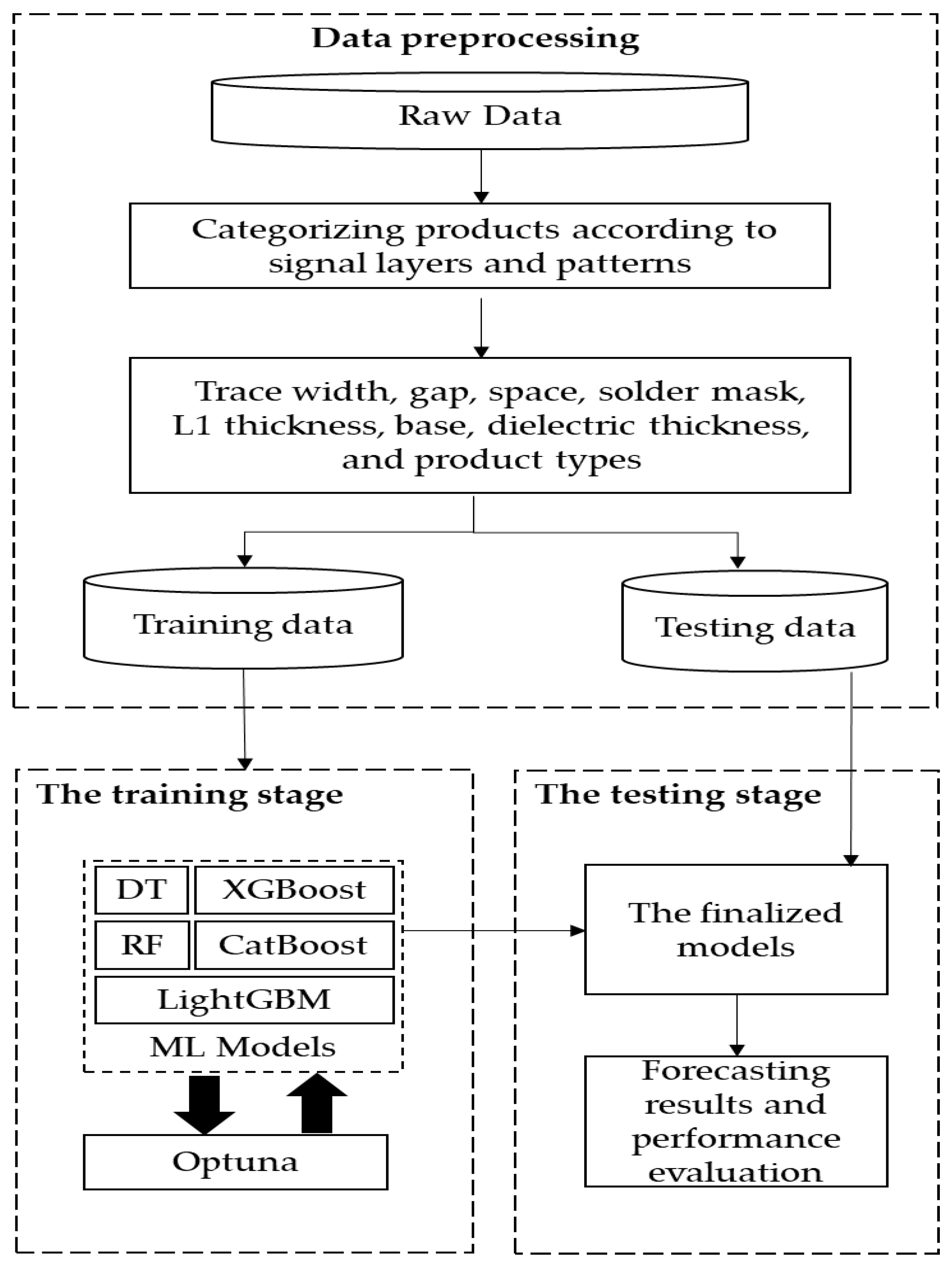
3. Tree-Based Machine Learning Architecture to Predict Impedance Value
3.1. Data Preprocessing
3.2. Tree-Based Machine Learning
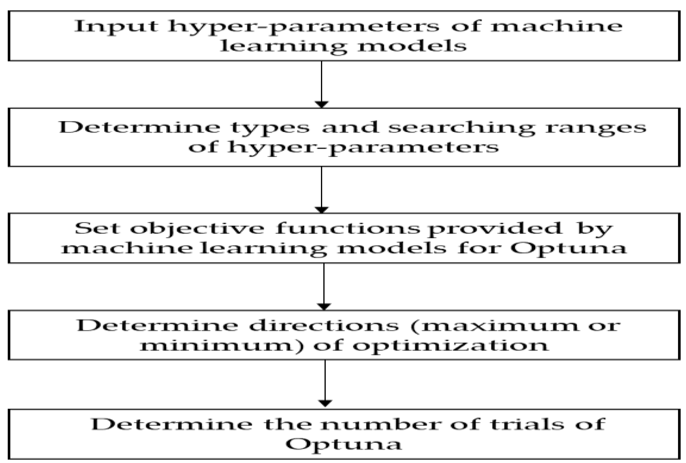
3.3. Optuna for Selecting Hyperparameters of Tree-Based Machine Learning Models
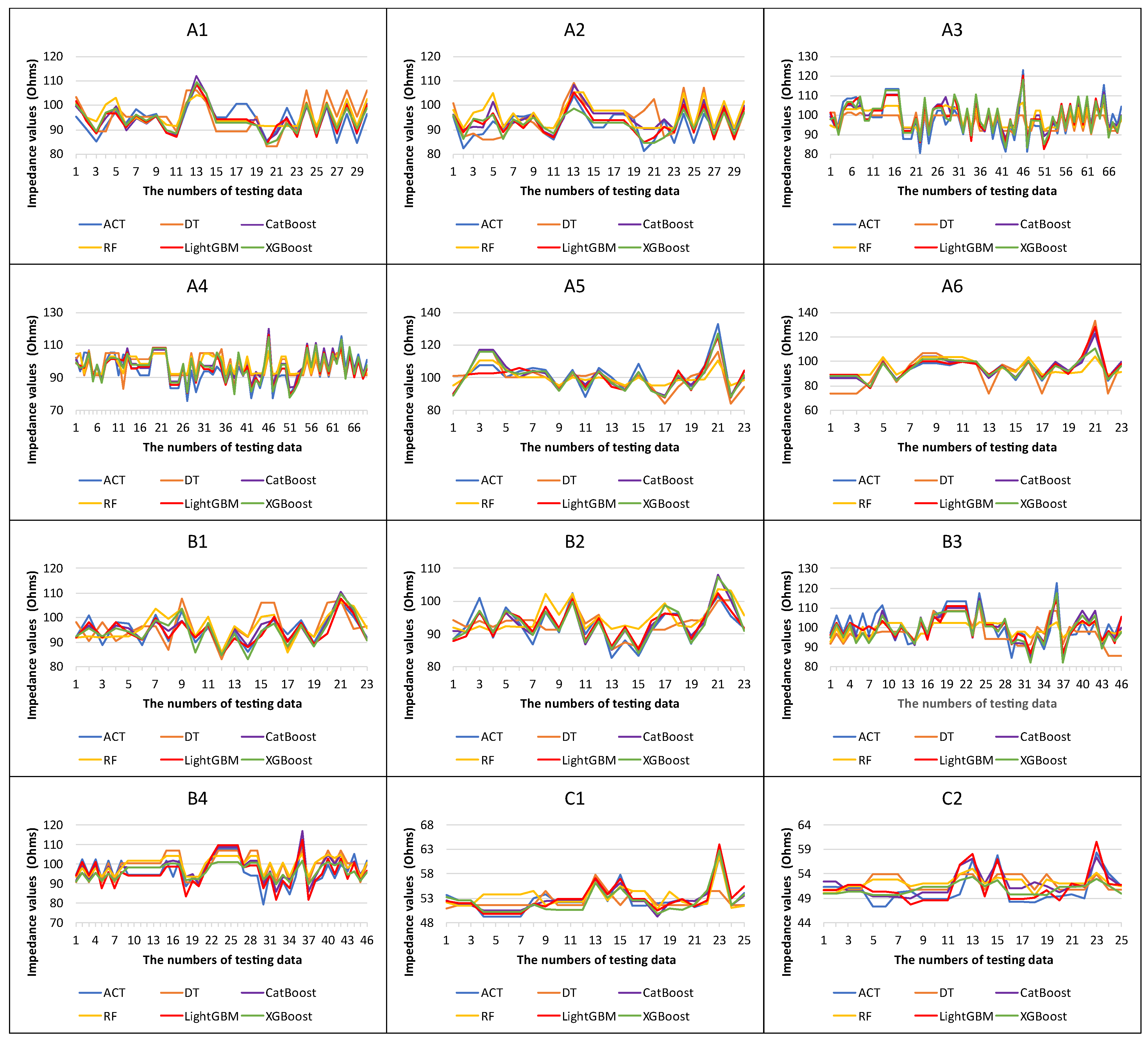
4. Numerical Results
5. Conclusions
Author Contributions
Funding
Institutional Review Board Statement
Informed Consent Statement
Data Availability Statement
Acknowledgments
Conflicts of Interest
References
- Wang, T.-C.; Zheng, Y.-G. Effective dielectric constant method for trace impedance control. In Proceedings of the 2008 International Conference on Electronic Packaging Technology & High Density Packaging, Shanghai, China, 28–31 July 2008; IEEE: Hoboken, NJ, USA, 2008; pp. 1–3. [Google Scholar]
- Jing, J.; Lingwen, K. Study of signal integrity for pcb level. In Proceedings of the 2010 11th International Conference on Electronic Packaging Technology & High Density Packaging, Xi’an, China, 16–19 August 2010; IEEE: Hoboken, NJ, USA, 2010; pp. 828–833. [Google Scholar]
- Zhang, J.W.; Chua, E.K.; See, K.Y.; Koh, W.J.; Chang, W.Y. Pre-layout multi-layer pdn model for high-speed board. In Proceedings of the 2016 Asia-Pacific International Symposium on Electromagnetic Compatibility (APEMC), Shenzhen, China, 18–21 May 2016; IEEE: Hoboken, NJ, USA, 2016; pp. 269–272. [Google Scholar]
- Shan, A.; Prakash, V. Certain investigation on impedance control of high speed signals in printed circuit board. In Proceedings of the 2022 International Conference on Inventive Computation Technologies (ICICT), Lalitpur, Nepal, 20–22 July 2022; IEEE: Hoboken, NJ, USA, 2022; pp. 564–569. [Google Scholar]
- Barzdenas, V.; Vasjanov, A. A method of optimizing characteristic impedance compensation using cut-outs in high-density pcb designs. Sensors 2022, 22, 964. [Google Scholar] [CrossRef]
- Wang, Y.; Dong, G.; Xiong, W.; Song, D.; Zhu, Z.; Yang, Y. Impedance modeling and analysis of multi-stacked on-chip power distribution network in 3D ICs. J. Comput. Electron. 2022, 21, 1282–1292. [Google Scholar] [CrossRef]
- Zhang, L.; Juang, J.; Kiguradze, Z.; Pu, B.; Jin, S.; Wu, S.; Yang, Z.; Fan, J.; Hwang, C. Fast impedance prediction for power distribution network using deep learning. Int. J. Numer. Model. Electron. Netw. Devices Fields 2022, 35, e2956. [Google Scholar] [CrossRef]
- Juang, J.; Zhang, L.; Kiguradze, Z.; Pu, B.; Jin, S.; Hwang, C. A modified genetic algorithm for the selection of decoupling capacitors in pdn design. In Proceedings of the 2021 IEEE International Joint EMC/SI/PI and EMC Europe Symposium, Virtual, 26 July–20 August 2021; IEEE: Hoboken, NJ, USA, 2021; pp. 712–717. [Google Scholar]
- Xu, Z.; Wang, Z.; Sun, Y.; Hwang, C.; Delingette, H.; Fan, J. Jitter-aware economic pdn optimization with a genetic algorithm. IEEE Trans. Microw. Theory Tech. 2021, 69, 3715–3725. [Google Scholar] [CrossRef]
- Park, H.; Park, J.; Kim, S.; Cho, K.; Lho, D.; Jeong, S.; Park, S.; Park, G.; Sim, B.; Kim, S.; et al. Deep reinforcement learning-based optimal decoupling capacitor design method for silicon interposer-based 2.5-D/3-D ICs. IEEE Trans. Compon. Packag. Manuf. Technol. 2020, 10, 467–478. [Google Scholar] [CrossRef]
- Swaminathan, M.; Torun, H.M.; Yu, H.; Hejase, J.A.; Becker, W.D. Demystifying machine learning for signal and power integrity problems in packaging. IEEE Trans. Compon. Packag. Manuf. Technol. 2020, 10, 1276–1295. [Google Scholar] [CrossRef]
- Cecchetti, R.; de Paulis, F.; Olivieri, C.; Orlandi, A.; Buecker, M. Effective pcb decoupling optimization by combining an iterative genetic algorithm and machine learning. Electronics 2020, 9, 1243. [Google Scholar] [CrossRef]
- Schierholz, M.; Yang, C.; Roy, K.; Swaminathan, M.; Schuster, C. Comparison of collaborative versus extended artificial neural networks for pdn design. In Proceedings of the 2020 IEEE 24th Workshop on Signal and Power Integrity (SPI), Cologne, Germany, 17–20 May 2020; IEEE: Hoboken, NJ, USA, 2020; pp. 1–4. [Google Scholar]
- Zhang, L.; Zhang, Z.; Huang, C.; Deng, H.; Lin, H.; Tseng, B.-C.; Drewniak, J.; Hwang, C. Decoupling capacitor selection algorithm for pdn based on deep reinforcement learning. In Proceedings of the 2019 IEEE International Symposium on Electromagnetic Compatibility, Signal & Power Integrity (EMC+SIPI), New Orleans, LA, USA, 22–26 July 2019; IEEE: Hoboken, NJ, USA, 2019; pp. 616–620. [Google Scholar]
- Park, H.; Park, J.; Lho, D.; Kim, S.; Jeong, S.; Park, G.; Kim, S.; Kang, H.; Sim, B.; Son, K.; et al. Fast and accurate deep neural network (dnn) model extension method for signal integrity (si) applications. In Proceedings of the 2019 Electrical Design of Advanced Packaging and Systems (EDAPS), Kaohsiung, Taiwan, 16–18 December 2019; IEEE: Hoboken, NJ, USA, 2019; pp. 1–3. [Google Scholar]
- Givaki, K.; Seyedzadeh, S.; Givaki, K. Machine learning based impedance estimation in power system. In Proceedings of the 8th Renewable Power Generation Conference (RPG 2019), Shanghai, China, 24–25 October 2019; IET: Lucknow, India, 2019; pp. 1–6. [Google Scholar]
- de Paulis, F.; Cecchetti, R.; Olivieri, C.; Piersanti, S.; Orlandi, A.; Buecker, M. Efficient iterative process based on an improved genetic algorithm for decoupling capacitor placement at board level. Electronics 2019, 8, 1219. [Google Scholar] [CrossRef] [Green Version]
- Renbi, A.; Carlson, J.; Delsing, J. Impact of pcb manufacturing process variations on trace impedance. In Proceedings of the International Symposium on Microelectronics, Long Beach, CA, USA, 9–13 October 2011; International Microelectronics Assembly and Packaging Society: Pittsburgh, PA, USA, 2008; pp. 000891–000895. [Google Scholar]
- Brist, G.A.; Krieger, J.; Willis, D. Pcb trace impedance: Impact of localized pcb copper density. In Proceedings of the IPC Apex Expo, San Diego, CA, USA, 28 February–1 March 2012. [Google Scholar]
- Wu, T.-L.; Buesink, F.; Canavero, F. Overview of signal integrity and emc design technologies on pcb: Fundamentals and latest progress. IEEE Trans. Electromagn. Compat. 2013, 55, 624–638. [Google Scholar]
- Rakhra, M.; Soniya, P.; Tanwar, D.; Singh, P.; Bordoloi, D.; Agarwal, P.; Takkar, S.; Jairath, K.; Verma, N. Crop price prediction using random forest and decision tree regression: A review. Mater. Today Proc. 2021; in press. [Google Scholar]
- Azimi, H.; Shiri, H.; Mahdianpari, M. Iceberg-seabed interaction evaluation in clay seabed using tree-based machine learning algorithms. J. Pipeline Sci. Eng. 2022, 2, 100075. [Google Scholar] [CrossRef]
- Iban, M.C. An explainable model for the mass appraisal of residences: The application of tree-based machine learning algorithms and interpretation of value determinants. Habitat Int. 2022, 128, 102660. [Google Scholar] [CrossRef]
- Kim, B.-Y.; Lim, Y.-K.; Cha, J.W. Short-term prediction of particulate matter (pm10 and pm2.5) in seoul, south korea using tree-based machine learning algorithms. Atmos. Pollut. Res. 2022, 13, 101547. [Google Scholar] [CrossRef]
- Sadorsky, P. Forecasting solar stock prices using tree-based machine learning classification: How important are silver prices? N. Am. J. Econ. Financ. 2022, 61, 101705. [Google Scholar] [CrossRef]
- Xiaosong, Z.; Qiangfu, Z. Stock prediction using optimized lightgbm based on cost awareness. In Proceedings of the 2021 5th IEEE International Conference on Cybernetics (CYBCONF), Virtual, 8–10 June 2021; IEEE: Hoboken, NJ, USA, 2021; pp. 107–113. [Google Scholar]
- Zhang, N.; Gao, C.; Xiao, M. Lightgbm stock forecasting model based on pca. In Proceedings of the 2021 2nd International Seminar on Artificial Intelligence, Networking and Information Technology (AINIT), Shanghai, China, 15–17 October 2021; IEEE: Hoboken, NJ, USA, 2021; pp. 396–399. [Google Scholar]
- Funk, K.D.; Paul, H.L.; Philips, A.Q. Point break: Using machine learning to uncover a critical mass in women’s representation. Political Sci. Res. Methods 2022, 10, 372–390. [Google Scholar] [CrossRef]
- Dong, S.; Fei, D. Improve the interpretability by decision tree regression: Exampled by an insurance dataset. In Proceedings of the 2021 International Conference on Computer Engineering and Artificial Intelligence (ICCEAI), Shanghai, China, 27–29 August 2021; IEEE: Hoboken, NJ, USA, 2021; pp. 325–330. [Google Scholar]
- Sohail, M.; Peres, P.; Li, Y. Feature importance analysis for customer management of insurance products. In Proceedings of the 2021 International Joint Conference on Neural Networks (IJCNN), Virtual, 18–22 July 2021; IEEE: Hoboken, NJ, USA, 2021; pp. 1–8. [Google Scholar]
- Aswad, F.M.; Kareem, A.N.; Khudhur, A.M.; Khalaf, B.A.; Mostafa, S.A. Tree-based machine learning algorithms in the internet of things environment for multivariate flood status prediction. J. Intell. Syst. 2022, 31, 1–14. [Google Scholar] [CrossRef]
- Demir, S.; Sahin, E.K. Comparison of tree-based machine learning algorithms for predicting liquefaction potential using canonical correlation forest, rotation forest, and random forest based on cpt data. Soil Dyn. Earthq. Eng. 2022, 154, 107130. [Google Scholar] [CrossRef]
- Ghiasi, M.M.; Zendehboudi, S. Application of decision tree-based ensemble learning in the classification of breast cancer. Comput. Biol. Med. 2021, 128, 104089. [Google Scholar] [CrossRef]
- Simsekler, M.C.E.; Rodrigues, C.; Qazi, A.; Ellahham, S.; Ozonoff, A. A comparative study of patient and staff safety evaluation using tree-based machine learning algorithms. Reliab. Eng. Syst. Saf. 2021, 208, 107416. [Google Scholar] [CrossRef]
- Luo, H.; Cheng, F.; Yu, H.; Yi, Y. Sdtr: Soft decision tree regressor for tabular data. IEEE Access 2021, 9, 55999–56011. [Google Scholar] [CrossRef]
- Li, M.; Vanberkel, P.; Zhong, X. Predicting ambulance offload delay using a hybrid decision tree model. Socio-Econ. Plan. Sci. 2022, 80, 101146. [Google Scholar] [CrossRef]
- Silva, G.; Schulze, B.; Ferro, M. Performance and Energy Efficiency Analysis of Machine Learning Algorithms towards Green AI: A Case Study of Decision Tree Algorithms. Master’s Thesis, National Laboratory for Scientific Computing, Petrópolis, Brazil, 2021. [Google Scholar]
- García, E.M.; Alberti, M.G.; Arcos Álvarez, A.A. Measurement-while-drilling based estimation of dynamic penetrometer values using decision trees and random forests. Appl. Sci. 2022, 12, 4565. [Google Scholar] [CrossRef]
- Khiem, N.M.; Takahashi, Y.; Yasuma, H.; Dong, K.T.P.; Hai, T.N.; Kimura, N. A novel machine learning approach to predict the export price of seafood products based on competitive information: The case of the export of vietnamese shrimp to the us market. PloS ONE 2022, 17, e0275290. [Google Scholar] [CrossRef] [PubMed]
- Breiman, L. Random forests. Mach. Learn. 2001, 45, 5–32. [Google Scholar] [CrossRef] [Green Version]
- Fan, G.-F.; Yu, M.; Dong, S.-Q.; Yeh, Y.-H.; Hong, W.-C. Forecasting short-term electricity load using hybrid support vector regression with grey catastrophe and random forest modeling. Util. Policy 2021, 73, 101294. [Google Scholar] [CrossRef]
- Khrakhuean, W.; Chutima, P. Real-time induction motor health index prediction in a petrochemical plant using machine learning. Eng. J. 2022, 26, 91–107. [Google Scholar] [CrossRef]
- Chen, T.; Guestrin, C. Xgboost: A scalable tree boosting system. In Proceedings of the 22nd ACM SIGKDD International Conference on Knowledge Discovery and Data Mining, San Francisco, CA, USA, 13–17 August 2016; pp. 785–794. [Google Scholar]
- Ali, H.A.; Mohamed, C.; Abdelhamid, B.; Ourdani, N.; El Alami, T. A comparative evaluation use bagging and boosting ensemble classifiers. In Proceedings of the 2022 International Conference on Intelligent Systems and Computer Vision (ISCV), Fez, Morocco, 18–20 May 2022; IEEE: Hoboken, NJ, USA, 2022; pp. 1–6. [Google Scholar]
- Guang, M.; Yan, C.; Liu, G.; Wang, J.; Jiang, C. A novel neighborhood-weighted sampling method for imbalanced datasets. Chin. J. Electron. 2022, 31, 969–979. [Google Scholar] [CrossRef]
- Hancock, J.; Khoshgoftaar, T.M. Performance of catboost and xgboost in medicare fraud detection. In Proceedings of the 2020 19th IEEE International Conference on Machine Learning and Applications (ICMLA), Miami, FL, USA, 14–17 December 2020; IEEE: Hoboken, NJ, USA, 2020; pp. 572–579. [Google Scholar]
- Huang, Z.; Yang, M.; Yang, B.; Liu, W.; Chen, Z. Data-driven model for predicting production periods in the sagd process. Petroleum 2022, 8, 363–374. [Google Scholar] [CrossRef]
- Prokhorenkova, L.; Gusev, G.; Vorobev, A.; Dorogush, A.V.; Gulin, A. Catboost: Unbiased boosting with categorical features. Adv. Neural Inf. Process. Syst. 2018, 31. [Google Scholar]
- Winkelmolen, F.; Ivkin, N.; Bozkurt, H.F.; Karnin, Z. Practical and sample efficient zero-shot hpo. arXiv 2020. [Google Scholar] [CrossRef]
- Bassi, A.; Shenoy, A.; Sharma, A.; Sigurdson, H.; Glossop, C.; Chan, J.H. Building energy consumption forecasting: A comparison of gradient boosting models. In Proceedings of the 12th International Conference on Advances in Information Technology, Bangkok, Thailand, 29 June–1 July 2021; pp. 1–9. [Google Scholar]
- Zheng, J.; Hu, M.; Wang, C.; Wang, S.; Han, B.; Wang, H. Spatial patterns of residents’ daily activity space and its influencing factors based on the catboost model: A case study of nanjing, china. Front. Archit. Res. 2022, 11, 1193–1204. [Google Scholar] [CrossRef]
- Ke, G.; Meng, Q.; Finley, T.; Wang, T.; Chen, W.; Ma, W.; Ye, Q.; Liu, T.-Y. LightGBM: A highly efficient gradient boosting decision tree. Adv. Neural Inf. Process. Syst. 2017, 30. [Google Scholar]
- Tang, M.; Zhao, Q.; Ding, S.X.; Wu, H.; Li, L.; Long, W.; Huang, B. An improved lightgbm algorithm for online fault detection of wind turbine gearboxes. Energies 2020, 13, 807. [Google Scholar] [CrossRef] [Green Version]
- Gan, M.; Pan, S.; Chen, Y.; Cheng, C.; Pan, H.; Zhu, X. Application of the machine learning lightgbm model to the prediction of the water levels of the lower columbia river. J. Mar. Sci. Eng. 2021, 9, 496. [Google Scholar] [CrossRef]
- Liang, S.; Peng, J.; Xu, Y.; Ye, H. Passive fetal movement recognition approaches using hyperparameter tuned lightgbm model and bayesian optimization. Comput. Intell. Neurosci. 2021, 2021, 6252362. [Google Scholar] [CrossRef]
- Le, H.; Peng, B.; Uy, J.; Carrillo, D.; Zhang, Y.; Aevermann, B.D.; Scheuermann, R.H. Machine learning for cell type classification from single nucleus rna sequencing data. PloS ONE 2022, 17, e0275070. [Google Scholar] [CrossRef]
- Andonie, R. Hyperparameter optimization in learning systems. J. Membr. Comput. 2019, 1, 279–291. [Google Scholar] [CrossRef] [Green Version]
- Yang, L.; Shami, A. On hyperparameter optimization of machine learning algorithms: Theory and practice. Neurocomputing 2020, 415, 295–316. [Google Scholar] [CrossRef]
- Akiba, T.; Sano, S.; Yanase, T.; Ohta, T.; Koyama, M. Optuna: A next-generation hyperparameter optimization framework. In Proceedings of the 25th ACM SIGKDD International Conference on Knowledge Discovery & Data Mining, Anchorage, AK, USA, 4–8 August 2019; pp. 2623–2631. [Google Scholar]
- Chintakindi, S.; Alsamhan, A.; Abidi, M.H.; Kumar, M.P. Annealing of monel 400 alloy using principal component analysis, hyper-parameter optimization, machine learning techniques, and multi-objective particle swarm optimization. Int. J. Comput. Intell. Syst. 2022, 15, 18. [Google Scholar] [CrossRef]
- Sipper, M. High per parameter: A large-scale study of hyperparameter tuning for machine learning algorithms. Algorithms 2022, 15, 315. [Google Scholar] [CrossRef]
- Lewis, C.D. Industrial and Business Forecasting Methods: A Practical Guide to Exponential Smoothing and Curve Fitting (p40); Butterworth-Heinemann: Oxford, UK, 1982. [Google Scholar]
- Calisto, F.M.; Nunes, N.; Nascimento, J.C. Modeling adoption of intelligent agents in medical imaging. Int. J. Hum.-Comput. Stud. 2022, 168, 102922. [Google Scholar] [CrossRef]
- Hematian, H.; Ranjbar, E. Evaluating urban public spaces from mental health point of view: Comparing pedestrian and car-dominated streets. J. Transp. Health 2022, 27, 101532. [Google Scholar] [CrossRef]
- Moon, J.; Lee, J.; Lee, S.; Yun, H. Urban river dissolved oxygen prediction model using machine learning. Water 2022, 14, 1899. [Google Scholar] [CrossRef]


| Literature | Years | Applications | Methods |
|---|---|---|---|
| Zhang et al. [7] | 2022 | Impedance prediction | DNN |
| Juang et al. [8] | 2022 | Decoupling capacitor | Genetic Algorithms |
| Xu et al. [9] | 2021 | Decoupling placement optimization | Genetic Algorithms |
| Park et al. [10] | 2020 | Decoupling capacitor | Q-Learning |
| Swaminathan et al. [11] | 2020 | Signal and power integrity | FFNN, RNN, CNN |
| Cecchetti et al. [12] | 2020 | Decoupling capacitor | GA-ANN |
| Schierholz et al. [13] | 2020 | Predicting target impedance violations | ANN |
| Zhang et al. [14] | 2019 | Decoupling capacitor | DRL, DNN |
| Park et al. [15] | 2019 | Signal and power integrity | DNN |
| Givaki et al. [16] | 2019 | Impedance estimation | Random Forest |
| Paulis et al. [17] | 2019 | Decoupling placement optimization | Genetic Algorithms |
| Product Categories | Patterns | Attributes (Variables) | ||||||
|---|---|---|---|---|---|---|---|---|
| X1 | X2 | X3 | X4 | X5 | X6 | X7 | ||
| Trace Width (um) | Gap (um) | Space (um) | Solder Mask (um) | L1 Thickness (um) | Base (um) | DielectricThickness (um) | ||
| A | GSSG | X | X | X | X | X | X | X |
| B | SS | X | X | X | X | X | X | |
| C | S | X | X | X | X | X | ||
| Product Subcategories | Signal Layers | Patterns | Instances |
|---|---|---|---|
| A1 | Base | GSSG | 146 |
| A2 | L1 | GSSG | 146 |
| A3 | Base | GSSG | 343 |
| A4 | L1 | GSSG | 342 |
| A5 | Base | GSSG | 114 |
| A6 | L1 | GSSG | 113 |
| B1 | Base | SS | 115 |
| B2 | L1 | SS | 115 |
| B3 | Base | SS | 229 |
| B4 | L1 | SS | 228 |
| C1 | Base | S | 122 |
| C2 | L1 | S | 122 |
| Hyperparameters | Implications | Types | Search Ranges |
|---|---|---|---|
| splitter | The strategy used for choosing the division. | Categorical numbers | ‘best’, ‘random’ |
| max_depth | The maximum depth of the tree. | Integers | 2, 24 |
| min_samples_split | The minimum number of samples required to split an internal node. | Integers | 2, 9 |
| max_features | The number of features to consider when looking for the best split | Categorical numbers | ‘sqrt’, ‘auto’, ‘log2’ |
| max_leaf_nodes | Grow a tree with max_leaf_nodes in best-first fashion. | Integers | 10, 1000 |
| Hyperparameters | Implications | Types | Search Ranges |
|---|---|---|---|
| n_estimators | The number of trees in the forest. | Integers | 50, 1000 |
| max_depth | The maximum depth of the tree. | Integers | 2, 24 |
| min_samples_split | The minimum number of data points in a node before the node is split. | Integers | 2, 9 |
| Hyper-Parameter | Implication | Types | Search Ranges |
|---|---|---|---|
| lambda | L2 regularization term on weights. | Real numbers | 0.00001, 10 |
| alpha | L1 regularization term on weights. | Real numbers | 0.00001, 10 |
| colsample_bytree | The subsample ratio of columns when constructing each tree. | Real numbers | 0.2, 0.6 |
| subsample | The subsample ratio of the training instances. | Real numbers | 0.4, 0.8 |
| learning_rate | The learning rate. | Real numbers | 0.0001, 0.2 |
| n_estimators | The number of trees. | Integers | 50, 10,000 |
| max_depth | The maximum depth of a tree. | Integers | 2, 12 |
| min_child_weight | The minimum sum of instance weight (hessian) needed in a child. | Integers | 1, 300 |
| Hyper-Parameter | Implication | Types | Search Ranges |
|---|---|---|---|
| iterations | The maximum number of trees. | Integers | 50, 10,000 |
| depth | The maximum depth of the tree. | Integers | 2, 12 |
| learning_rate | The learning rate. | Real numbers | 0.0001, 0.2 |
| l2_leaf_reg | Coefficient at the L2 regularization term of the cost function. | Real numbers | 0.00001, 10 |
| bagging_temperature | Defines the settings of the Bayesian bootstrap. | Real numbers | 0.01, 10 |
| min_child_samples (min_data_in_leaf) | The minimum number of training samples in a leaf. | Integers | 5, 100 |
| Hyperparameters | Implications | Types | Search Ranges |
|---|---|---|---|
| n_estimators | The number of trees. | Integers | 50, 10,000 |
| learning_rate | The learning rate. | Real numbers | 0.0001, 0.2 |
| num_leaves | The number of leaves per tree. | Integers | 2, 2048 |
| max_depth | The maximum learning depth. | Integers | 2, 12 |
| min_data_in_leaf | The minimal number of data in one leaf. Prevent overfitting. | Integers | 1, 100 |
| lambda_l1 | L1 regularization. Prevent overfitting. | Real numbers | 0.00001, 10 |
| lambda_l2 | L2 regularization. Prevent overfitting. | Real numbers | 0.00001, 10 |
| min_gain_to_split | The minimal error reduction to conduct the further split. | Real numbers | 0, 15 |
| bagging_fraction | The ratio of the selected data to the total data. | Real numbers | 0.3, 1.0 |
| bagging_freq | Frequency of re-sampling the data when bagging_fraction is smaller than 1.0. | Integers | 1, 7 |
| feature_fraction | The proportion of the selected feature to the total number of features. | Real numbers | 0.3, 1.0 |
| extra_trees | Uses randomized trees. | Categorical numbers | ‘True’, ‘False’ |
| Methods | Hyperparameters | A1 | A2 | A3 | A4 | A5 | A6 |
|---|---|---|---|---|---|---|---|
| DT | splitter | random | random | random | random | random | random |
| max_depth | 5 | 19 | 3 | 3 | 11 | 15 | |
| min_samples_split | 8 | 3 | 8 | 3 | 9 | 5 | |
| max_features | sqrt | log2 | log2 | log2 | sqrt | sqrt | |
| max_leaf_nodes | 730 | 886 | 604 | 359 | 279 | 778 | |
| FrozenTrial # | 41 | 31 | 85 | 45 | 77 | 21 | |
| FR | n_estimators | 50 | 273 | 140 | 184 | 328 | 60 |
| max_depth | 2 | 2 | 2 | 2 | 2 | 2 | |
| min_samples_split | 5 | 4 | 2 | 3 | 9 | 9 | |
| FrozenTrial # | 76 | 53 | 13 | 60 | 93 | 12 | |
| XGBoost | lambda | 0.00013 | 9.99880 | 7.39058 | 0.03166 | 0.33494 | 0.00003 |
| alpha | 0.17368 | 0.11708 | 0.00006 | 4.42219 | 0.31300 | 1.30132 | |
| colsample_bytree | 0.53136 | 0.43740 | 0.47339 | 0.50856 | 0.59988 | 0.31599 | |
| subsample | 0.72083 | 0.68340 | 0.58809 | 0.71827 | 0.50646 | 0.72486 | |
| learning_rate | 0.02817 | 0.02235 | 0.16934 | 0.03755 | 0.00503 | 0.00407 | |
| n_estimators | 3502 | 8701 | 3107 | 1555 | 3314 | 7162 | |
| max_depth | 3 | 4 | 2 | 10 | 3 | 4 | |
| min_child_weight | 3 | 1 | 1 | 5 | 1 | 1 | |
| FrozenTrial # | 27 | 80 | 96 | 14 | 87 | 52 | |
| CatBoost | iterations | 1361 | 1428 | 4808 | 7459 | 5246 | 9659 |
| depth | 2 | 11 | 4 | 10 | 4 | 7 | |
| learning_rate | 0.16536 | 0.02557 | 0.14240 | 0.00447 | 0.01723 | 0.01481 | |
| l2_leaf_reg | 0.00031 | 0.00052 | 0.00003 | 0.00037 | 3.60489 | 0.00001 | |
| bagging_temperature | 0.01262 | 3.30881 | 0.06255 | 1.54283 | 3.77145 | 0.06189 | |
| min_child_samples | 48 | 25 | 29 | 45 | 49 | 49 | |
| FrozenTrial # | 94 | 14 | 72 | 5 | 82 | 57 | |
| LightGBM | n_estimators | 6775 | 7866 | 4876 | 8457 | 7635 | 1355 |
| learning_rate | 0.12735 | 0.19625 | 0.17452 | 0.13543 | 0.16941 | 0.18596 | |
| num_leaves | 649 | 1631 | 1599 | 517 | 19 | 1150 | |
| max_depth | 12 | 8 | 10 | 6 | 7 | 4 | |
| min_data_in_leaf | 6 | 10 | 1 | 6 | 3 | 3 | |
| lambda_l1 | 0.65465 | 0.40568 | 0.10117 | 4.44552 | 0.01356 | 0.30749 | |
| lambda_l2 | 0.02067 | 7.10369 | 0.00002 | 3.64057 | 0.00007 | 0.00032 | |
| min_gain_to_split | 0.62324 | 6.27989 | 8.02722 | 0.01769 | 0.51251 | 3.25957 | |
| bagging_fraction | 0.71382 | 0.66880 | 0.55024 | 0.78785 | 0.73125 | 0.84466 | |
| bagging_freq | 5 | 1 | 3 | 7 | 3 | 2 | |
| feature_fraction | 0.97166 | 0.36366 | 0.84806 | 0.81182 | 0.79440 | 0.57880 | |
| extra_trees | TRUE | FALSE | TRUE | FALSE | TRUE | FALSE | |
| FrozenTrial # | 41 | 82 | 71 | 30 | 82 | 92 |
| Methods | Hyperparameters | B1 | B2 | B3 | B4 | C5 | C6 |
|---|---|---|---|---|---|---|---|
| DT | splitter | random | best | Best | random | random | best |
| max_depth | 17 | 8 | 14 | 3 | 2 | 2 | |
| min_samples_split | 3 | 2 | 9 | 6 | 7 | 3 | |
| max_features | sqrt | log2 | log2 | sqrt | sqrt | log2 | |
| max_leaf_nodes | 371 | 522 | 280 | 228 | 894 | 41 | |
| FrozenTrial # | 19 | 40 | 96 | 78 | 10 | 70 | |
| FR | n_estimators | 107 | 115 | 273 | 410 | 609 | 66 |
| max_depth | 2 | 2 | 2 | 2 | 2 | 2 | |
| min_samples_split | 5 | 9 | 5 | 2 | 8 | 6 | |
| FrozenTrial # | 45 | 11 | 99 | 98 | 85 | 15 | |
| XGBoost | lambda | 0.10002 | 0.02107 | 0.35943 | 0.00057 | 0.00014 | 3.33129 |
| alpha | 0.00025 | 0.02653 | 0.01639 | 5.60999 | 0.48286 | 0.01335 | |
| colsample_bytree | 0.57253 | 0.53535 | 0.35838 | 0.23654 | 0.53890 | 0.53090 | |
| subsample | 0.58380 | 0.72630 | 0.40557 | 0.79891 | 0.40926 | 0.69241 | |
| learning_rate | 0.02778 | 0.02027 | 0.16094 | 0.02471 | 0.00655 | 0.01433 | |
| n_estimators | 2002 | 2416 | 2905 | 9578 | 5672 | 2965 | |
| max_depth | 12 | 3 | 2 | 10 | 5 | 7 | |
| min_child_weight | 1 | 1 | 1 | 2 | 3 | 8 | |
| FrozenTrial # | 78 | 99 | 78 | 48 | 6 | 91 | |
| CatBoost | iterations | 5168 | 8064 | 5747 | 3031 | 2759 | 7897 |
| depth | 11 | 4 | 4 | 11 | 6 | 8 | |
| learning_rate | 0.01978 | 0.02600 | 0.12381 | 0.02291 | 0.00251 | 0.06970 | |
| l2_leaf_reg | 0.00001 | 0.18489 | 0.00003 | 0.07952 | 0.00251 | 0.00017 | |
| bagging_temperature | 1.11136 | 0.13162 | 0.62528 | 0.22679 | 0.23521 | 1.79410 | |
| min_child_samples | 77 | 74 | 49 | 81 | 89 | 65 | |
| FrozenTrial # | 90 | 87 | 91 | 23 | 17 | 92 | |
| LightGBM | n_estimators | 4130 | 2450 | 8692 | 8417 | 5671 | 3523 |
| learning_rate | 0.12182 | 0.17747 | 0.17526 | 0.19914 | 0.16131 | 0.18101 | |
| num_leaves | 670 | 924 | 1757 | 153 | 207 | 1683 | |
| max_depth | 12 | 5 | 9 | 10 | 3 | 3 | |
| min_data_in_leaf | 1 | 1 | 12 | 3 | 9 | 2 | |
| lambda_l1 | 0.00268 | 0.00543 | 0.02561 | 0.13634 | 0.00013 | 0.20529 | |
| lambda_l2 | 0.01191 | 0.23902 | 0.11103 | 0.02720 | 0.00183 | 0.00008 | |
| min_gain_to_split | 4.40312 | 1.28234 | 0.03857 | 4.66666 | 5.22525 | 0.41965 | |
| bagging_fraction | 0.40501 | 0.95348 | 0.84419 | 0.91639 | 0.64485 | 0.41063 | |
| bagging_freq | 7 | 2 | 1 | 6 | 1 | 5 | |
| feature_fraction | 0.77680 | 0.49448 | 0.89466 | 0.61959 | 0.92896 | 0.90923 | |
| extra_trees | FALSE | FALSE | FALSE | TRUE | FALSE | TRUE | |
| FrozenTrial # | 24 | 29 | 61 | 19 | 56 | 99 |
| Dataset | DT | RF | XGB | CatBoost | LightGBM | Average |
|---|---|---|---|---|---|---|
| with Optuna | ||||||
| MAPE | ||||||
| A1 | 5.36% | 4.38% | 3.19% | 2.77% | 2.74% | 3.68% |
| A2 | 5.42% | 5.17% | 3.32% | 3.63% | 3.12% | 4.13% |
| A3 | 4.64% | 4.80% | 3.25% | 3.64% | 3.25% | 3.92% |
| A4 | 6.89% | 6.45% | 3.85% | 4.15% | 3.46% | 4.96% |
| A5 | 5.36% | 5.36% | 2.59% | 3.10% | 2.20% | 3.72% |
| A6 | 6.25% | 5.27% | 1.81% | 1.77% | 1.38% | 3.29% |
| B1 | 5.38% | 4.11% | 2.59% | 2.16% | 1.99% | 3.25% |
| B2 | 3.27% | 4.48% | 2.18% | 2.37% | 1.99% | 2.86% |
| B3 | 6.04% | 5.30% | 3.58% | 3.33% | 2.99% | 4.25% |
| B4 | 5.31% | 5.87% | 4.88% | 3.72% | 2.67% | 4.49% |
| C1 | 3.54% | 3.38% | 2.31% | 1.86% | 1.69% | 2.56% |
| C2 | 5.40% | 5.41% | 3.99% | 3.49% | 2.67% | 4.19% |
| Average | 5.24% | 5.00% | 3.13% | 3.00% | 2.51% | 3.78% |
| RMSE | ||||||
| A1 | 6.12 | 4.79 | 3.64 | 3.19 | 3.17 | 4.18 |
| A2 | 6.44 | 5.73 | 3.53 | 4.20 | 3.31 | 4.64 |
| A3 | 6.34 | 5.73 | 3.67 | 4.23 | 3.55 | 4.71 |
| A4 | 8.05 | 7.27 | 4.39 | 4.60 | 4.09 | 5.68 |
| A5 | 6.94 | 6.99 | 3.59 | 4.35 | 3.20 | 5.02 |
| A6 | 7.58 | 6.89 | 3.86 | 2.23 | 1.45 | 4.40 |
| B1 | 5.88 | 4.65 | 2.94 | 2.40 | 2.36 | 3.65 |
| B2 | 3.84 | 4.86 | 2.67 | 2.66 | 2.21 | 3.25 |
| B3 | 7.40 | 7.00 | 4.31 | 4.10 | 3.84 | 5.33 |
| B4 | 6.05 | 6.56 | 5.39 | 4.22 | 3.28 | 5.10 |
| C1 | 2.53 | 2.32 | 1.46 | 1.16 | 1.11 | 1.72 |
| C2 | 3.36 | 3.13 | 2.39 | 2.13 | 1.90 | 2.58 |
| Average | 5.88 | 5.49 | 3.49 | 3.29 | 2.79 | 4.19 |
| R2 | ||||||
| A1 | −0.12 | 0.32 | 0.60 | 0.70 | 0.70 | 0.44 |
| A2 | −0.39 | −0.10 | 0.58 | 0.41 | 0.63 | 0.23 |
| A3 | 0.46 | 0.56 | 0.82 | 0.76 | 0.83 | 0.69 |
| A4 | 0.17 | 0.33 | 0.75 | 0.73 | 0.79 | 0.55 |
| A5 | 0.48 | 0.48 | 0.86 | 0.80 | 0.89 | 0.70 |
| A6 | 0.37 | 0.48 | 0.84 | 0.95 | 0.98 | 0.72 |
| B1 | −0.12 | 0.30 | 0.72 | 0.81 | 0.82 | 0.51 |
| B2 | 0.49 | 0.19 | 0.75 | 0.76 | 0.83 | 0.60 |
| B3 | 0.24 | 0.32 | 0.74 | 0.77 | 0.80 | 0.57 |
| B4 | 0.25 | 0.11 | 0.40 | 0.63 | 0.78 | 0.44 |
| C1 | 0.12 | 0.26 | 0.71 | 0.81 | 0.83 | 0.55 |
| C2 | −0.28 | −0.11 | 0.35 | 0.49 | 0.59 | 0.21 |
| Average | 0.14 | 0.26 | 0.68 | 0.72 | 0.79 | 0.52 |
Disclaimer/Publisher’s Note: The statements, opinions and data contained in all publications are solely those of the individual author(s) and contributor(s) and not of MDPI and/or the editor(s). MDPI and/or the editor(s) disclaim responsibility for any injury to people or property resulting from any ideas, methods, instructions or products referred to in the content. |
© 2023 by the authors. Licensee MDPI, Basel, Switzerland. This article is an open access article distributed under the terms and conditions of the Creative Commons Attribution (CC BY) license (https://creativecommons.org/licenses/by/4.0/).
Share and Cite
Lai, J.-P.; Lin, Y.-L.; Lin, H.-C.; Shih, C.-Y.; Wang, Y.-P.; Pai, P.-F. Tree-Based Machine Learning Models with Optuna in Predicting Impedance Values for Circuit Analysis. Micromachines 2023, 14, 265. https://doi.org/10.3390/mi14020265
Lai J-P, Lin Y-L, Lin H-C, Shih C-Y, Wang Y-P, Pai P-F. Tree-Based Machine Learning Models with Optuna in Predicting Impedance Values for Circuit Analysis. Micromachines. 2023; 14(2):265. https://doi.org/10.3390/mi14020265
Chicago/Turabian StyleLai, Jung-Pin, Ying-Lei Lin, Ho-Chuan Lin, Chih-Yuan Shih, Yu-Po Wang, and Ping-Feng Pai. 2023. "Tree-Based Machine Learning Models with Optuna in Predicting Impedance Values for Circuit Analysis" Micromachines 14, no. 2: 265. https://doi.org/10.3390/mi14020265