Classification and Identification of Contaminants in Recyclable Containers Based on a Recursive Feature Elimination-Light Gradient Boosting Machine Algorithm Using an Electronic Nose

Abstract

Establishing an excellent recycling mechanism for containers is of great importance for environmental protection, so many technical approaches applied during the whole recycling stage have become popular research issues. Among them, classification is considered a key step, but this work is mostly achieved manually in practical applications. Due to the influence of human subjectivity, the classification accuracy often varies significantly. In order to overcome this shortcoming, this paper proposes an identification method based on a Recursive Feature Elimination-Light Gradient Boosting Machine (RFE-LightGBM) algorithm using electronic nose. Firstly, odor features were extracted, and feature datasets were then constructed based on the response data of the electronic nose to the detected gases. Afterwards, a principal component analysis (PCA) and the RFE-LightGBM algorithm were applied to reduce the dimensionality of the feature datasets, and the differences between these two methods were analyzed, respectively. Finally, the differences in the classification accuracies on the three datasets (the original feature dataset, PCA dimensionality reduction dataset, and RFE-LightGBM dimensionality reduction dataset) were discussed. The results showed that the highest classification accuracy of 95% could be obtained by using the RFE-LightGBM algorithm in the classification stage of recyclable containers, compared to the original feature dataset (88.38%) and PCA dimensionality reduction dataset (92.02%).

1. Introduction

The recycling of containers can not only effectively decrease the disposal pressure of waste and reduce environmental pollution, but can also provide a large number of job positions [1]. The recycling of containers involves a series of steps such as classification and identification, cleaning, drying, shredding, and regeneration. Of all these steps, classification is the most important [2,3], because recycling value will be effectively increased by classifying waste containers. However, many factors such as the container’s size [4], color [5], pose [6], shape [7], external damage [8], internal contamination [9], and material [10] make achieving highly accurate classification and identification very challenging.

At present, the classification and identification of containers are mainly carried out manually, and have the limitations of high cost and low efficiency [11,12]. Additionally, some residual toxic and harmful gases may exist in those containers, which could hurt human health [13,14]. In addition, the subjectivity of the inspector can lead to inconsistent results [15,16]. To solve the above-mentioned problems, research into identification methods based on intelligent devices has become a popular research domain in recent decades. For example, Wang et al. [17] classified plastic bottles with different position relationships and colors based on image recognition, but detection inside the containers was not considered, and the experimental platform required strict lighting conditions. Dimitris et al. [18] used an online cloud computing platform with a distributed architecture for solid waste classification; therefore, the response speed limited its application for fast detection. Zhang et al. [19] proposed a recyclable waste classification model based on the combination of image classification and deep learning, and confirmed that this model could improve classification results on the TrashNet dataset; however, this model required a very large amount of clear image data for training, and its reliability was unstable. Wang et al. [20] proposed an innovative design concept of a smart recycling system based on Extenics to solve conflicts in cosmetic container recycling, but different categories of cosmetic containers were not investigated in this study.

Using an electronic nose system is a promising approach to solving the problems of classification and identification of contaminants. Actually, electronic noses have been proven to be effective for the classification and identification of contaminant gases. For instance, Wen et al. [21] detected the odors of rotten fruits with the help of an electronic nose, and achieved efficient identification of fruit freshness. Savirio et al. [22] applied an electronic nose to pre-adhesive recognition of relevant pollutants on the surface of composite fiber-reinforced polymers (CFRP). Herrero et al. [23] used an electronic nose to classify and quantify different pollutant gases in the air. Zhang et al. [24] identified six indoor air pollutants (formaldehyde, benzene, toluene, carbon monoxide, ammonia, and nitrogen dioxide) as air quality indicators, and classified the data collected using an electronic nose. Liu et al. [25] proposed a non-destructive method for detecting peach fungal contamination using an electronic nose, and showed that the electronic nose has high discrimination accuracy. Mesías et al. [26] also used an electronic nose as the predictive tool for detecting the chemical pollutants in roasted almonds.

In this paper, a model based on the Recursive Feature Elimination-Light Gradient Boosting Machine (RFE-LightGBM) algorithm is proposed in the classification stage of contaminants for recyclable containers. Based on the experimental results of using the proposed model, the difference in the classification accuracies on three datasets (the original feature dataset, principal component analysis (PCA) dimensionality reduction dataset, and RFE-LightGBM dimensionality reduction dataset) was firstly investigated. Subsequently, the PCA method and RFE-LightGBM algorithm were applied to reduce the dimensionality of the feature dataset, and the differences between the two methods were analyzed, respectively. Finally, the classification accuracies on these three datasets were discussed as well.

2. Algorithm Theory

Figure 1 shows the flowchart of the contaminant classification model proposed in this paper, which mainly consists of three processes: the data collection process, data feature process, and classification and identification process.

2.1. Light Gradient Boosting Machine (LightGBM)

The main idea of the optimal feature splitting point in the LightGBM algorithm [27,28] is as follows:

Assuming a dataset containing M samples and N features is given, LightGBM is an integrated model composed of K basic models, where each basic model represents a tree (representing different categories). Therefore, the predicted output of the integrated model can be expressed as Formular (1):

$${\widehat{y}}_i=\varphi (x_i)={\displaystyle \sum _{K=1}^K{f}_k(x_i)}$$

(1)

where $x_i$ is the characteristic value of the gas sample, $f_k$ is the predicted value of the K-th tree, and ${\widehat{y}}_i$ represents the current predicted value. Equation (1) represents the sum of the predicted values of K regression trees (the weights of the leaf nodes divided according to the corresponding decision rules of the regression tree) given an input $x_i$. By iterating on each prediction tree and fitting the current difference to obtain the optimal model, we define the objective function as Formular (2):

$$\mathrm{target}={\displaystyle \sum _{i=1}^{m}l({\widehat{y}}_i,y_i)}+{\displaystyle \sum _{K=1}^K\mathrm{\Omega }(f_k)}$$

(2)

where $l({\widehat{y}}_i,y_i)$ is the loss function between the predicted value and the actual value. $\mathrm{\Omega }(f_k)$ represents the penalty term for the complexity of the model to balance the complexity of the model, and can be determined using Formular (3):

$$\mathrm{\Omega }(f_k)=\mu T+\frac{1}{2}\lambda {‖\omega ‖}^2$$

(3)

where μ and λ represent the penalty coefficient, T represents the number of leaf nodes for a given tree, and ||ω||² is the square of the number of nodes on each leaf (predicted to be of the same category). When training the K-th tree, the first two K-1 trees in the front are known, and the unknown is the K-th tree. That is, based on the known decision tree constructed earlier, the K-th tree is constructed, and the predicted value of the K-th tree is represented by Formular (4):

$${\widehat{y}}_i^{(k)}={\widehat{y}}_i^{(k-1)}+f_k(x_i)$$

(4)

Taking Formular (4) into Formular (2), Formular (5) can represent the new objective function obtained:

$$\mathrm{target}={\displaystyle \sum _{i=1}^{m}l({\widehat{y}}_i^{(k-1)}+f_k(x_i),y_i)+\mathrm{\Omega }(f_k)+C}$$

(5)

Then the second-order Taylor approximation formular can be used to expand the objective function, as shown in Formular (6):

$$\mathrm{target}={\displaystyle \sum _{i=1}^m\left[l({\widehat{y}}_i^{(k-1)},{\widehat{y}}_i)+g_i{f}_k(x_i)+\frac{1}{2}{h}_i{f}_k^2(x_i)\right]}+\mathrm{\Omega }(f_k)+C$$

(6)

where $g_i=\partial {\widehat{y}}^{(k-1)}{({\widehat{y}}^{(k-1)}-y_i)}^2,h_i={\partial }^2{\widehat{y}}^{(k-1)}{({\widehat{y}}^{(k-1)}-y_i)}^2$ in Formular (6) is the first derivative and the second derivative of the Loss function, respectively; the best classification characteristics are determined using Formular (7).

$${\omega }_j=-\frac{G_j}{H_j+\lambda }$$

(7)

$G_j={\displaystyle \sum _{i\in I_j}{g}_i,H_j={\displaystyle \sum _{i\in I_j}{h}_i}}$ The final objective function can be represented as follows:

$$\mathrm{target}=-\frac{1}{2}{\displaystyle \sum _{j=1}^T\frac{G_j^2}{H_j+\lambda }+\mu T}$$

(8)

Finally, the information gain of all features is determined according to Formular (9):

$$Gain=\frac{1}{2}\left[\frac{G_L^2}{H_L+\lambda }+\frac{G_R^2}{H_R+\lambda }-\frac{{\left(G_L+G_R\right)}^2}{H_L+H_R+\lambda }\right]-\mu$$

(9)

Among them, G_L + G_R = H_L + H_R is the left and right branch sample set, split based on the best feature. The larger the value of the gain, the more it can reduce the loss of the objective function after splitting. This method can sort features based on the ranking of information gain and select the feature with the highest gain as the optimal splitting point.

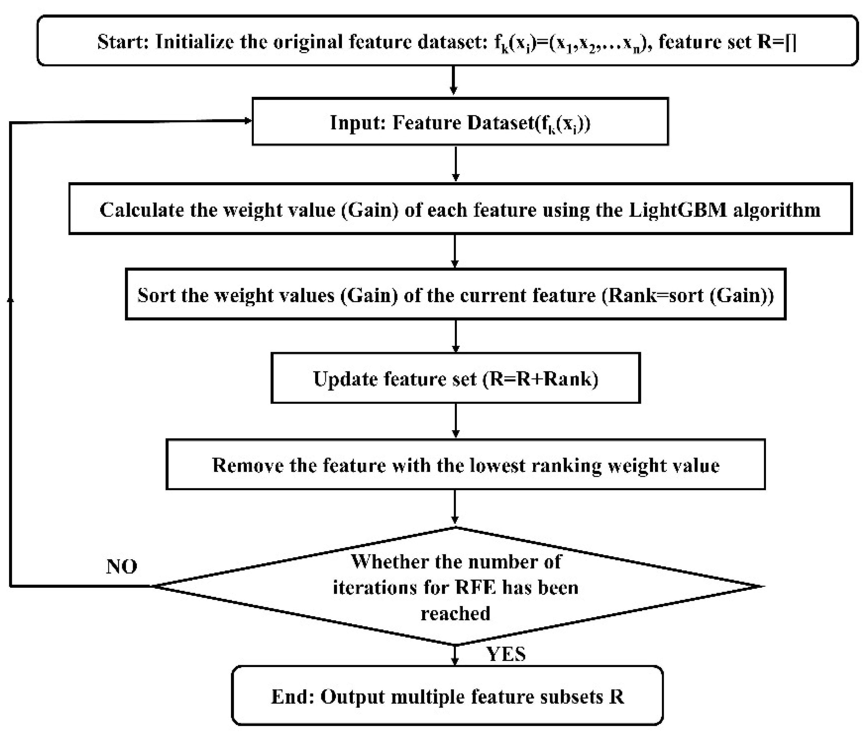
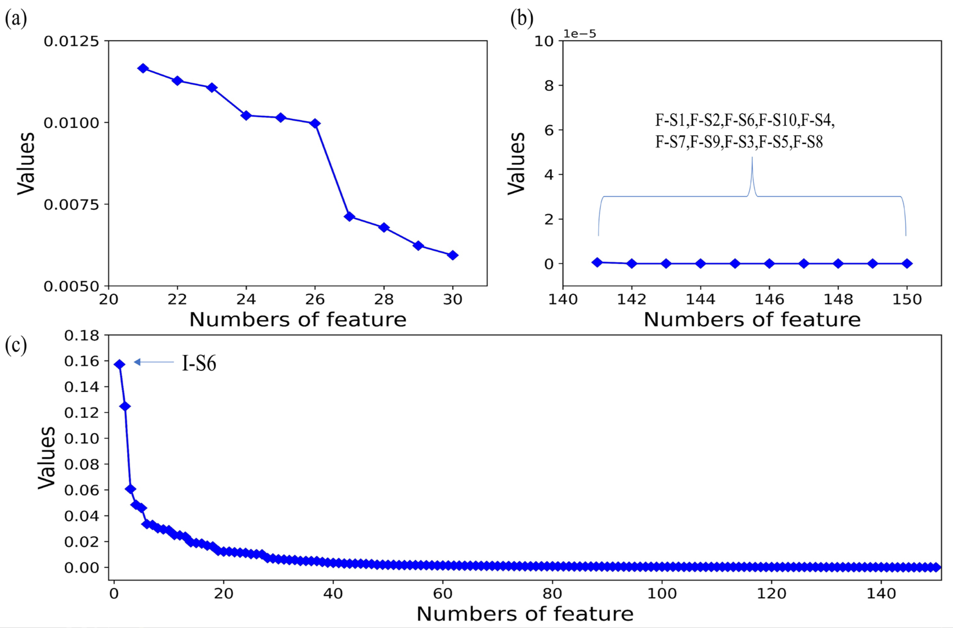
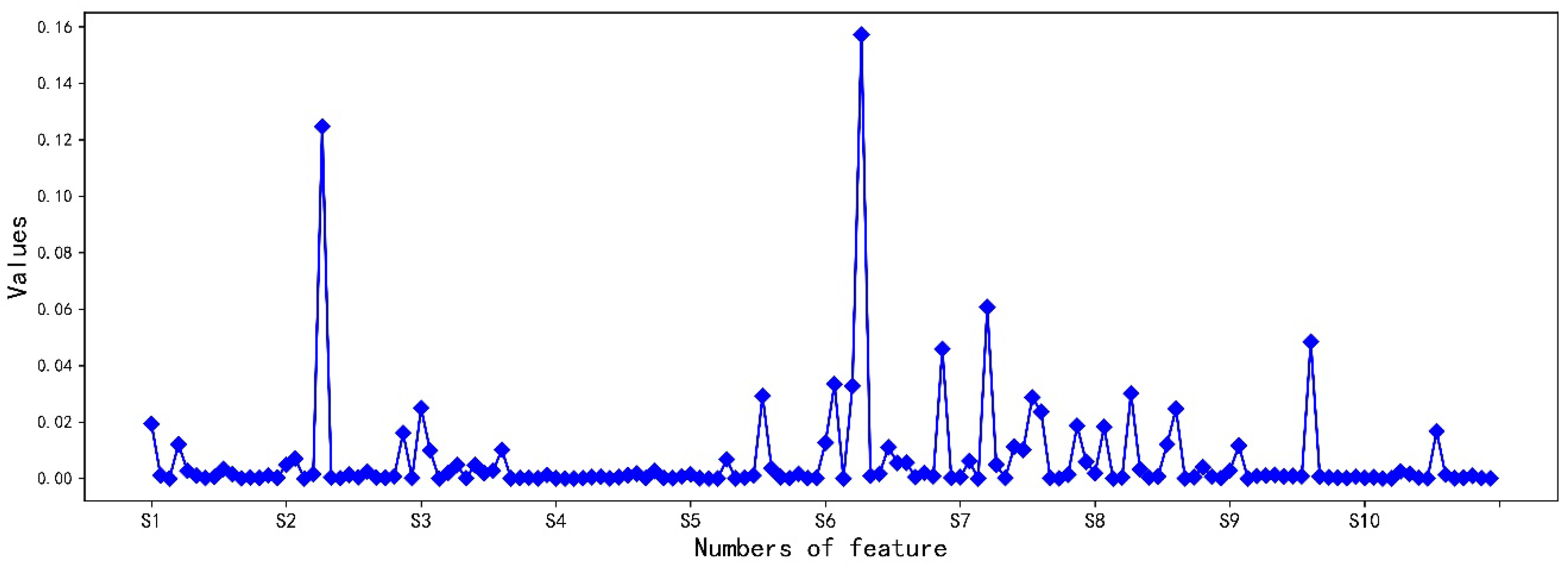
2.2. Recursive Feature Elimination-Light Gradient Boosting Machine (RFE-LightGBM) Feature Selection Algorithm

LightGBM was used as the base model for the feature recursive elimination algorithm to model the original dataset in this study. After the corresponding weight values were calculated, all features could be sorted according to their weight values. Then, the features with the lowest weight values were successively deleted from the feature dataset using recursive feature elimination (RFE) [29,30,31,32], and the features were iterated circularly (the iteration number is equal to the dimension of the original feature dataset). Finally, sorting tables related to the multiple feature weight values could be obtained. The feature selection algorithm based on RFE-LightGBM is shown in Figure 2.

2.3. Algorithm Evaluation Criteria

In order to obtain the optimal feature subset, the classification accuracy (ACC = (TP + TN)/(TP + TN + FP + FN)) [33] was used to evaluate the score of each feature subset. The feature subset with the highest accuracy score was chosen as the best feature dataset to verify the classification results of the test data obtained based on the proposed model.

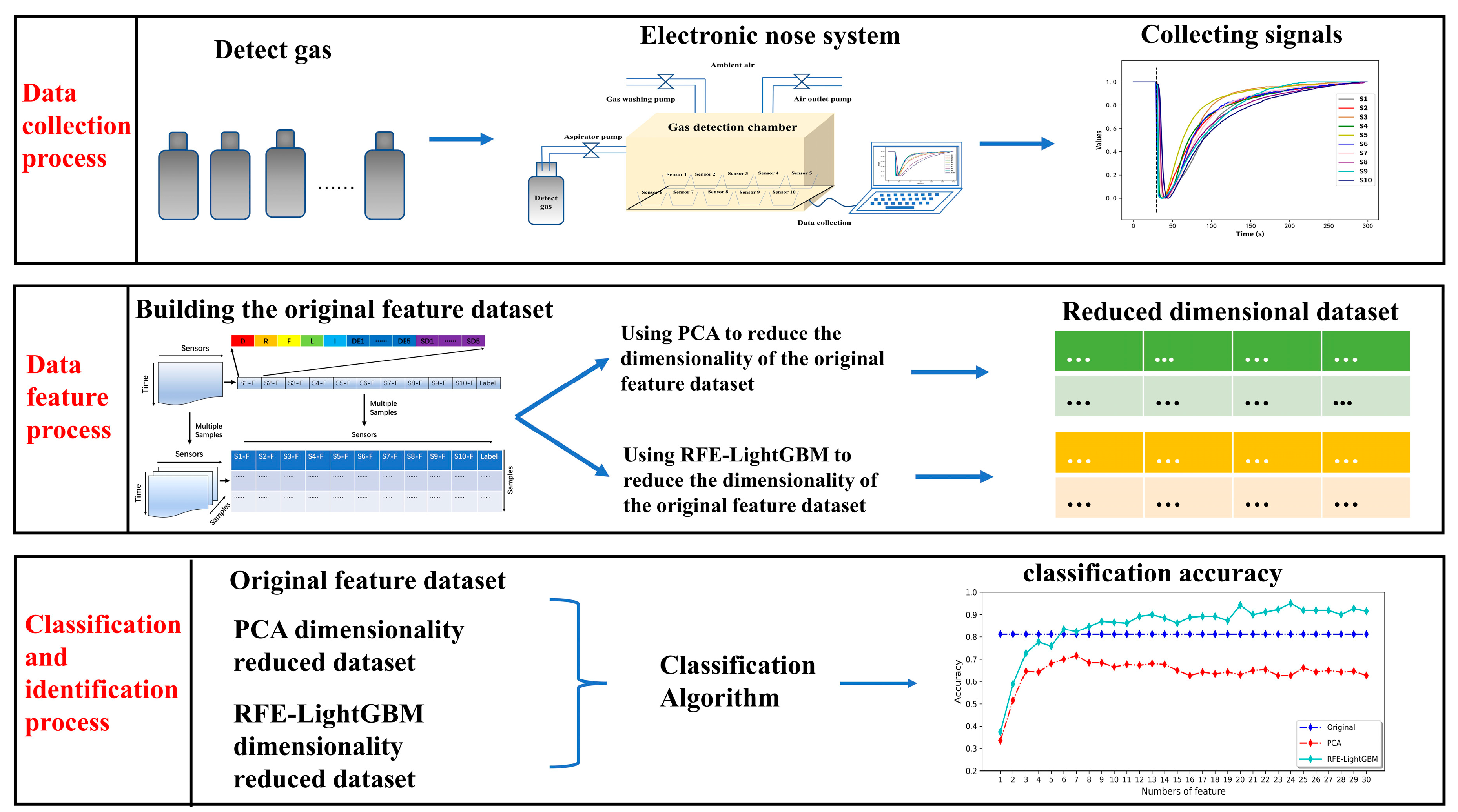
3. Materials and Methods

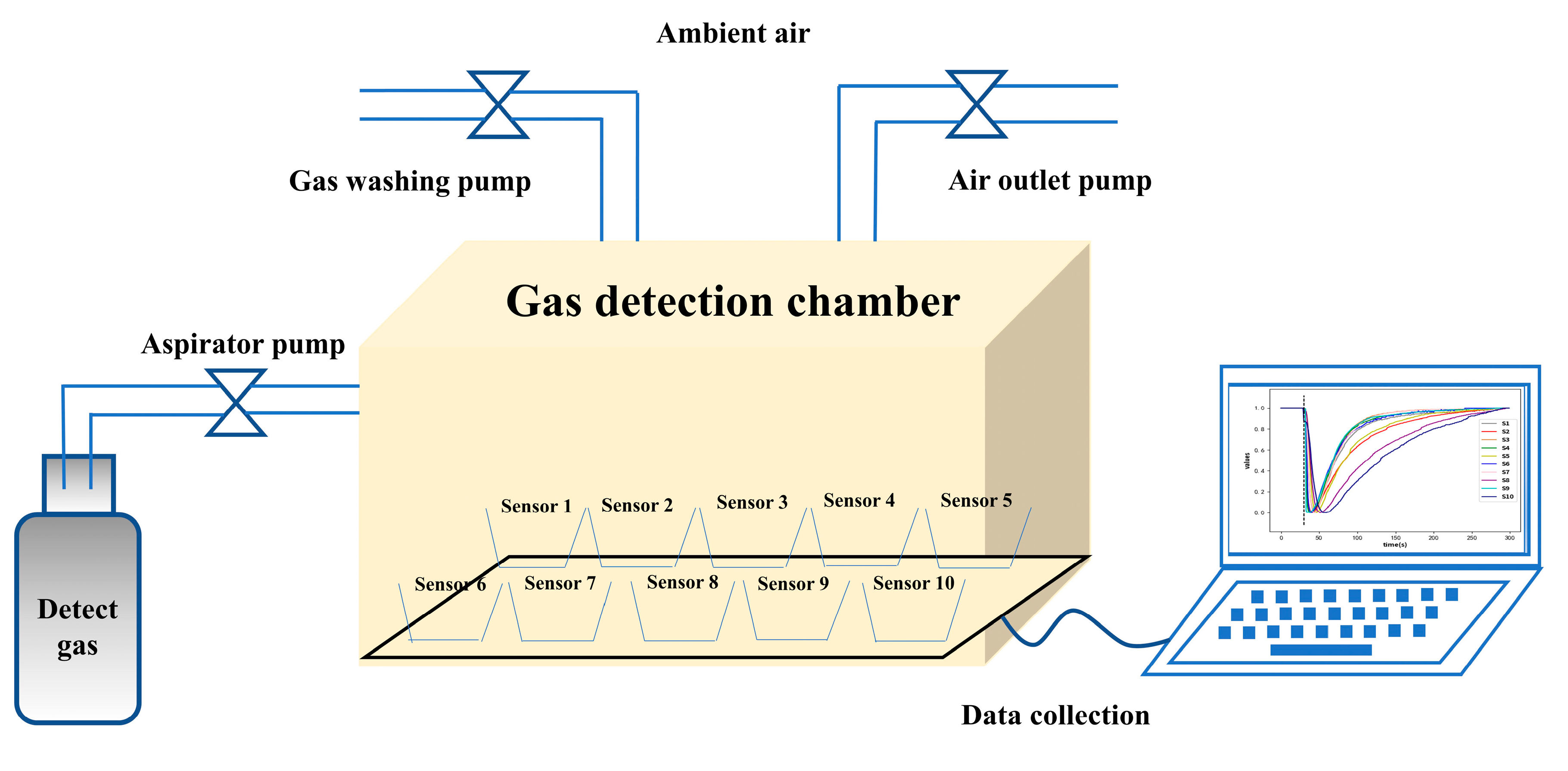
3.1. Electronic Nose System

Figure 3 shows the schematic of the electronic nose system used in this work, which consists of three components: a gas sensing array (10 homemade MEMS metal oxide sensors; because different sensors have different sensitivities to different gases, it is better to choose sensors with high sensitivity for different practical applications) [34,35]; a gas collection module; and a data acquisition module. The sensor parameters of the gas sensing array are listed in

Table 1. Characteristics of the employed sensors in the electronic nose system.

Sensor	Main Test Objects	Detection Range (ppm)	Response Time (s)
S1	Ethanol, Acetone, Hydrogen Sulfide	0.1–500	<20
S2	VOCs, Smog	1–500	<10
S3	Ethanol, Hydrogen Sulfide, Acetone	1–500	<20
S4	Hydrogen	0.1–300	<10
S5	Hydrogen Sulfide	0.5–300	<20
S6	Ammonia	10–300	<10
S7	Ethanol	1–500	<20
S8	VOCs	10–500	<20
S9	Hydrogen Sulfide, Carbon Monoxide	1–500	<10
S10	Acetone, Hydrogen Sulfide	0.1–500	<10

. The gas collection module is made of a 2L PE box and equipped with three pumps (the flow rate is approximately 800 mL/min). During the whole process of the experiment, the equipment, including the pumps, is controlled by a computer. The data acquisition module collects the response signal of the electronic nose to the detected gas and transfers it to the computer.

3.2. Experimental Procedures

In this work, barreled water buckets were used as recyclable containers. Under relatively fixed temperature and humidity conditions, the electronic nose system built in 3.1 was used to classify and identify contaminant gases in the recyclable container.

For 5 consecutive days, residual gases (cigarette butts, coffee, liquor, and vinegar) in 3 concentration levels (10%, 30%, 50%), and uncontaminated barrels (100%) were classified into 13 categories. Each category of gas was detected 20 times each day (all the substances to be detected were poured out from the containers before measurement), so that a total of 100 data were obtained for each category of gas sample. The contaminant (taking coffee as an example, representing the ratio of the coffee volume to the whole volume of a barreled water bucket) and the percentage concentration of the experimental sample (e.g., a concentration of 50% means the volume ratio of contaminant in the recyclable container before measurement, which is expressed as the gas concentration in the recyclable container) are listed in

Table 2. The composition and concentration of experimental sample gases.

Sample Label	Contaminant	Gas percentage Concentration
G0	Water	100%
G1	Cigarette	10%
G2	Cigarette	30%
G3	Cigarette	50%
G4	Coffee	10%
G5	Coffee	30%
G6	Coffee	50%
G7	Liquor	10%
G8	Liquor	30%
G9	Liquor	50%
G10	Vinegar	10%
G11	Vinegar	30%
G12	Vinegar	50%

. Details of the experimental procedure are as follows:

(1)

The sensing array was preheated for 30 s to bring the baseline sensor resistance values to a steady state.

(2)

The aspirator pump was turned on at the 30 s mark, and sent the gas to the detection chamber. The response signal of the sensor to the gas during the pumping time was collected.

(3)

The aspirator pump was turned off at the 35 s mark, and the gas washing pump and air outlet pump were turned on (purging the gas detection chamber with ambient air) until all sensor resistance values returned to the original baseline values.

(4)

Repeat the operations of steps 1–3 until data collection is completed for all target detectors.

4. Results

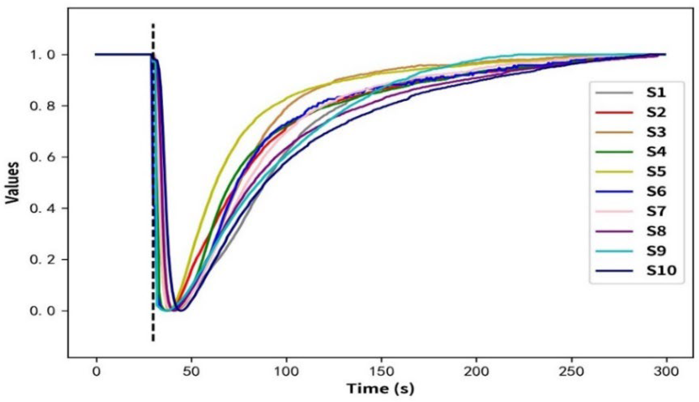
4.1. Response Curve of the Electronic Nose System

Affected by different sensitive materials, sensors will have different response sensitivities to the same target gas [36,37,38]. Moreover, environmental factors could also cause the baseline fluctuation of the sensors [39,40]. In order to eliminate these effects, we processed the collected signals according to the following formular:

$$values=\frac{x-\min (x)}{\max (x)-\min (x)}$$

(10)

where x, min (x), and max (x) represent all the original data of each sensor, the minimum, and the maximum value in the data, respectively. Figure 4 shows the result curve of the raw data processed according to Formular (10). The horizontal axis represents the detection time, and the vertical axis represents the value after the change in the original data. It can be observed that the sensor array reached a stable state during the preheating phase (0–30 s). When the gas enters the detection chamber (30 s: black dashed line), the resistance values of the sensor array will decrease with the increase in the concentration of the gas. After stopping the gas supply, the resistance values of the sensor array return to the initial steady state with time.

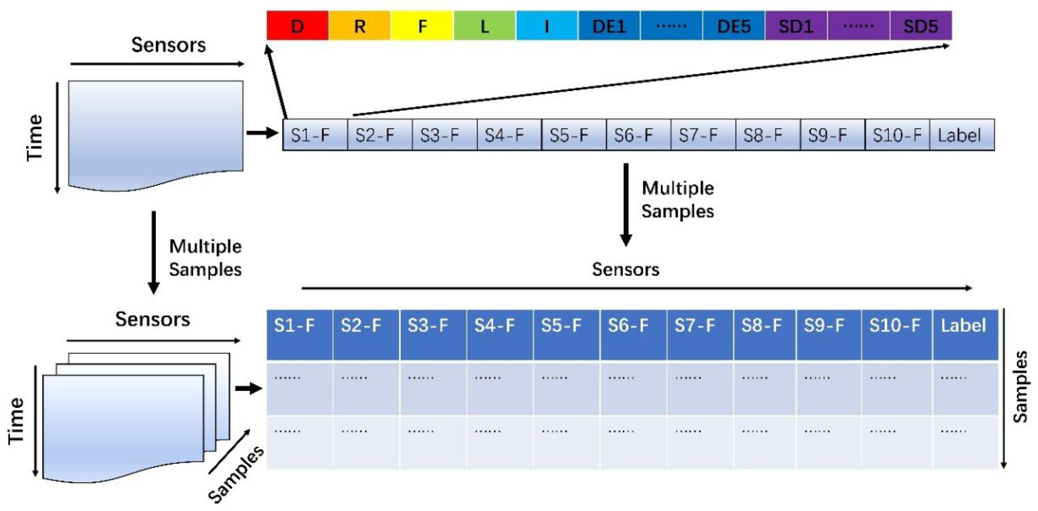
4.2. Feature Datasets Constructed by Manual Methods

In this study, we extracted four steady-state features and three transient features from the pre-processed signals of each sensor [41], with a total of 15 features (1 + 1 + 1 + 1 + 1 + 1 + 5 + 5 = 15). The features extracted from all sensors (10 in total) are represented by different colors, and all the features are connected in order to form a feature vector that includes 150 features (10 × 15 = 150). Additionally, all the sample feature vectors are stacked together to form a feature dataset, as shown in Figure 5. The data collected by each sensor during the pumping period were defined as xⁱ, and their detailed description is shown in the formular in

Table 3. Gas features extracted using manual methods.

Symbol Mark	Number	Feature Description	Function
D	1	Difference	$x_{\max }^i-x_{\min }^i$
R	1	Relative difference	$x_{\max }^i/x_{\min }^i$
F	1	Fractional difference	$(x_{\max }^i-x_{\min }^i)/x_{\min }^i$
L	1	Logarithm difference	$\log \left(x_{\max }^i/x_{\min }^i\right)$
I	1	Integral	${\displaystyle \underset{0}{\overset{5}{\int }}{x}^i(t)dt}$
DE	5	Derivative	$d{x}^i(t)/dt$
SD	5	Second derivative	$d^2{x}^i(t)/d{t}^2$

(where $x_{\max }^i,x_{\min }^i$ represent the maximum value and minimum value).

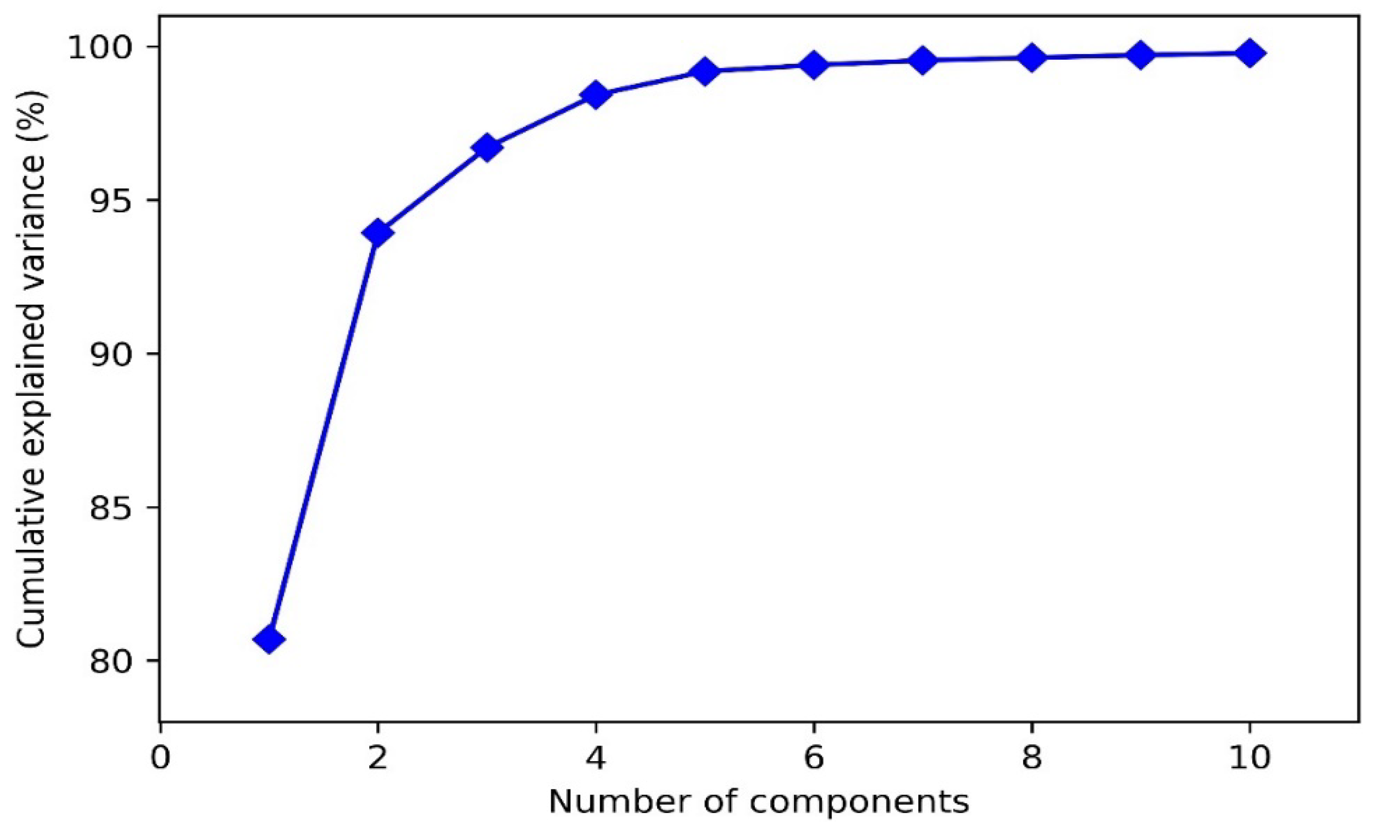
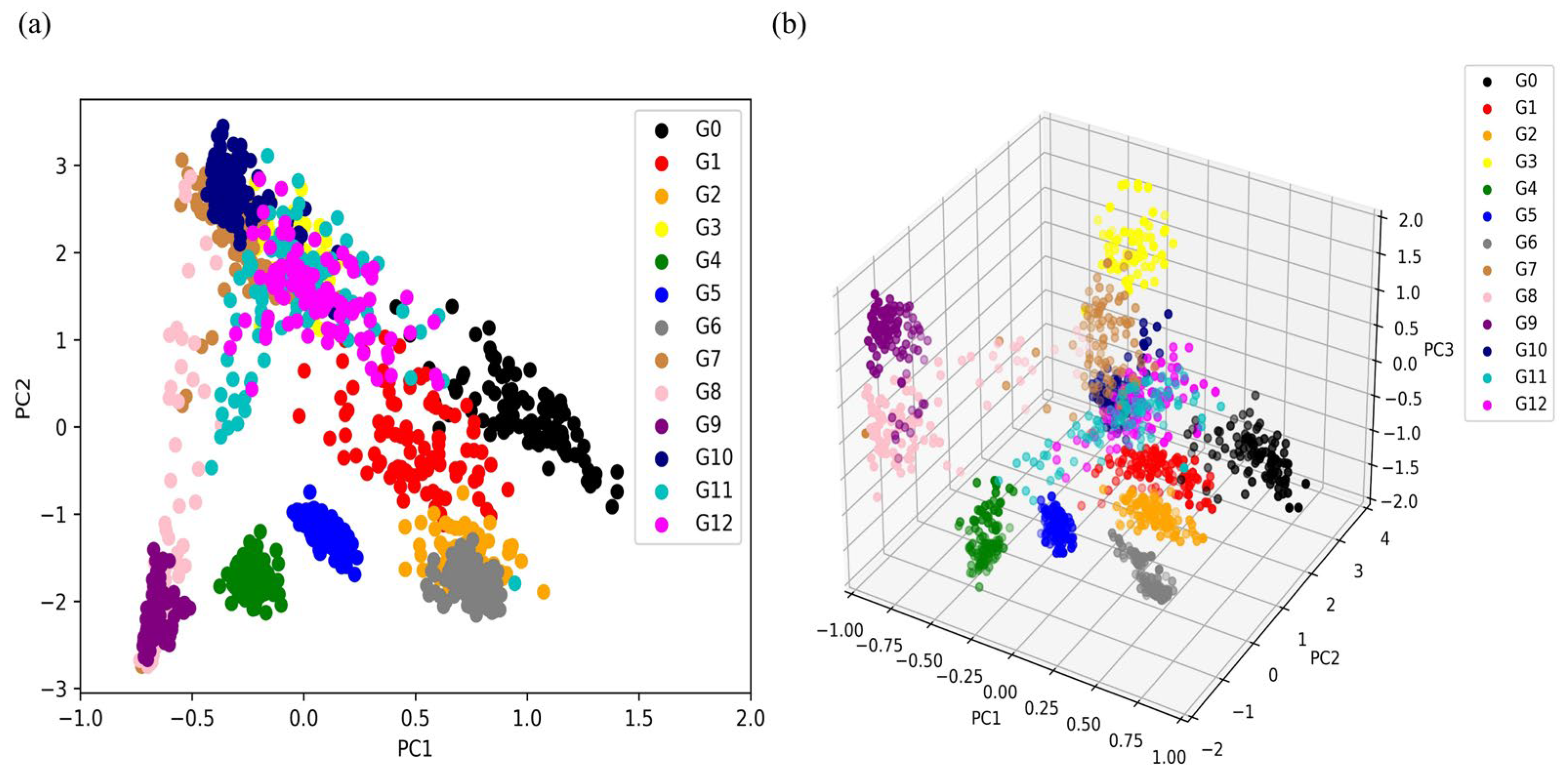
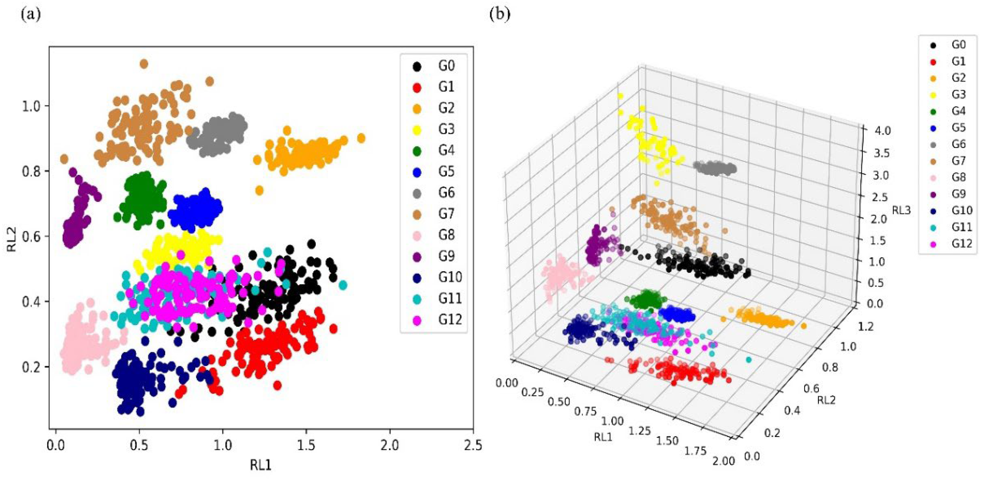
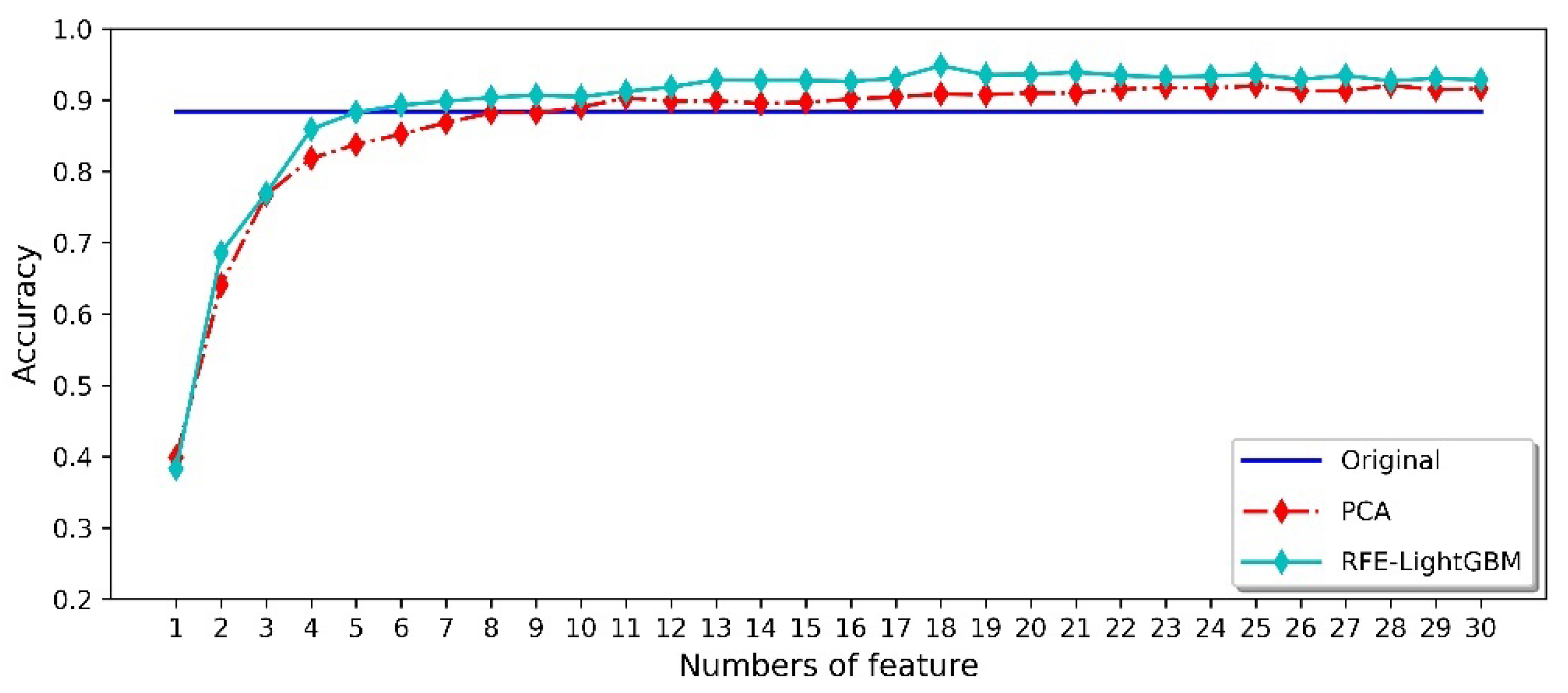
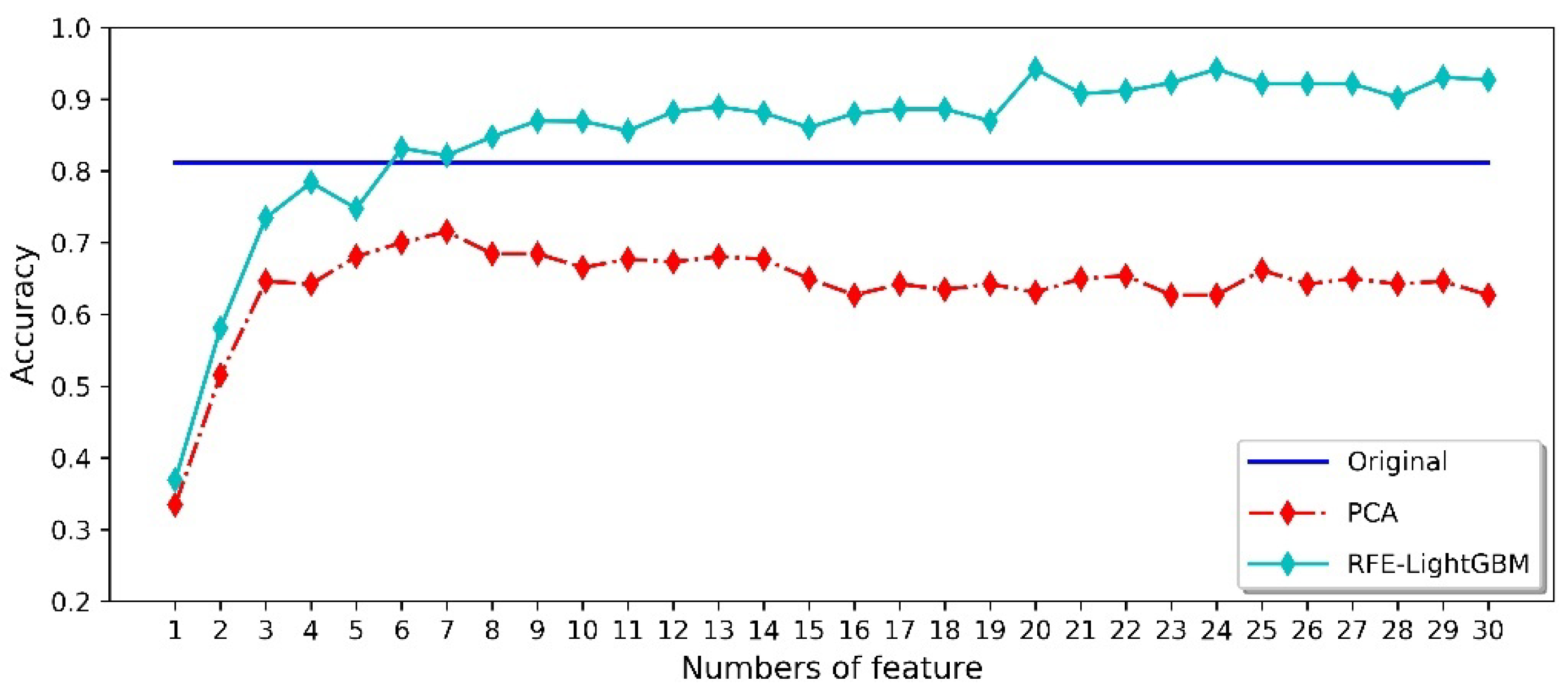
4.3. Dimensionality Reduction of Feature Datasets

The feature dataset constructed using the above method has high dimensionality (with each feature vector containing 150-dimensional features). In order to speed up the model training, pre-processing of the feature dataset is necessary for eliminating the redundant features before training.

In the field of gas identification, principal component analysis (PCA) is a widely used method [42]. Figure 6 shows the variance contribution of each principal component calculated using the PCA method, and the cumulative variance contribution of the first two and three principal components is 93.93% and 96.71%, respectively. When considering the first 10 principal components, the cumulative variance contribution could reach up to 99.78%.

Figure 7 shows the visualization results of the original feature dataset after dimensionality reduction using PCA. It can be observed that when only the first two principal components are focused, there is a large amount of overlap between different categories, indicating that PCA cannot classify well (Figure 7a). Figure 7b shows the sample visualization distribution when applying the first three principal components. Here, the displayed classification effect is more obvious. It can also be seen that the ability to distinguish different samples has improved, but there are still some overlapping samples.

Figure 8c shows the percentile weight values obtained using the RFE-LightGBM method for the features. The feature with the highest score is I-S6 (which is the integral feature of the sixth sensor), which means this feature provides the greatest information gain in classification. In contrast, as shown in Figure 8b, all the fractional difference feature contribution values were zero. This means that this type of feature is completely unhelpful for the classification. In addition, it can be seen in Figure 8a that only 26 features have contribution values higher than 0.01. Therefore, in order to reduce the dimensionality of the feature dataset, features with relatively low contribution rates could be discarded.

Table 4. Weight value details of the first 26 obtained features higher than 0.01, obtained using RFE-LightGBM analysis.

Feature Name	Importance
I-S6	0.1571
I-S2	0.1246
L-S7	0.0607
DE5-S9	0.0484
SD4-S6	0.0458
R-S6	0.0334
L-S6	0.0327
I-S8	0.0301
DE4-S5	0.0292
DE4-S7	0.0287
D-S3	0.0250
DE5-S8	0.0247
DE5-S7	0.0236
D-S1	0.0194
SD4-S7	0.0187
R-S8	0.0183
DE4-S10	0.0167
SD4-S2	0.0161
D-S6	0.0127
L-S1	0.0121
DE4-S8	0.0121
R-S9	0.0116
DE2-S7	0.0112
DE3-S6	0.0110
DE5-S3	0.0102
DE3-S7	0.0101
SUM	0.8442

shows 26 features with weight values greater than 0.01, with a total of 0.8442. Among them, integral features and derivative features made up a high proportion (17/26), which also indicates they make high contributions to gas identification. This shows that the integration features and derivative features can accurately express the information of the original data. Integral features can provide the best features, and derivative features can explain the rate and acceleration of the reaction. At the same time, the number of features formed by sensors S6, S7, and S8 correspond to 16/26. This shows that these features may have a significant impact on the classification and identification results. Therefore, the result confirms that the RFE-LightGBM method can utilize the original data information preserved in a small number of features in the model.

Figure 9 shows the importance score of each feature on different sensors. The larger values represent greater contributions to gas classification and identification. In addition, it can be seen that the feature weight of S4 is relatively low, which also indicates that S4 has a relatively small impact on the identification result. Therefore, removing S4 may not only reduce the amount of data generated and shorten the time for feature preprocessing, but also further reduce the power consumption of the sensor. In summary, the application of RFE-LightGBM in the field of gas identification not only effectively optimizes the sensing array, but also reduces the dimensionality of the feature dataset, thereby utilizing a small number of features to retain a large amount of original information.

The visualized distribution of samples obtained using the RFE-LightGBM feature selection method was shown in Figure 10. The distribution of samples in different categories using the first two features is shown in Figure 10a. Although there are still overlapping phenomena between different categories, it is obviously lower than PCA. The visualization using the first three features also yielded the same conclusion (Figure 10b). After using the RFE-LightGBM method for feature selection, the distinction between different samples is more obvious.

5. Discussion

In this paper, a BPNN (back propagation neural network) model with one hidden layer [43] was constructed as a classifier. The number of input layers was equal to features, the number of output layers was equal to categories, and the categories were labeled with one-hot coding. The number of neurons in the hidden layer was defined as 10, and sigmoid was used as the activation function. To prevent the overfitting of the model, a five-fold cross-validation was used in the training process.

In order to compare the influence of different feature processing methods on the final classification results, 80% of the data from three datasets (randomly divided among the original feature dataset, PCA dimensionality reduction dataset, and RFE-LightGBM dimensionality reduction dataset) were used for model training. The remaining data were used for model validation, and the results obtained are shown in Figure 11. The original feature dataset (1-150 dimensional features) obtained an average classification and identification accuracy of 88.38%. At the same time, one can also see that most PCA methods achieved lower accuracy than the RFE-LightGBM method. Compared with the PCA method, the RFE-LightGBM method can not only reduce the dimensions of the original feature dataset, but also obtain 94.84% classification accuracy using the first 18 features.

When performing gas identification, odors can change over time, which in turn is reflected by differences in the collected data. For example, Mahdi et al. [44] classified a variety of cheeses with different storage periods, Huang et al. [45] used RBF-ANN to assess fish freshness, and Madiha et al. [46] applied an electronic nose system for determining milk storage dates. The above studies have proved that the gas data collected on different days will affect the identification results. Therefore, when the electronic nose system is used to detect recyclable containers, the storage time of the contaminants in the containers will interfere with the final classification accuracy. If time interference can be overcome, the misclassification rate can be effectively reduced, and thus the robustness of the classification model can be significantly improved. Consequently, to explore the effect of gas data collected on different days on the classification and identification results, we divided the data into five schemes. We used different days of data as the training dataset and unknown days of data as the testing dataset, as shown in

Table 5. The datasets constructed according to the time of acquisition.

Datasets	Number of Days of Training Data Collection	Number of Days of Testing Data Collection
Scheme 1	2-3-4-5	1
Scheme 2	1-3-4-5	2
Scheme 3	1-2-4-5	3
Scheme 4	1-2-3-5	4
Scheme 5	1-2-3-4	5

.

The training and testing datasets were divided into five datasets (see Table 5) to compare the effect of different feature preprocessing methods on the final classification results of each scheme. Figure 12 shows the recognition accuracy of the Scheme 1 dataset. We used the original feature dataset of 1-150 dimensions to train the model, and obtained an average accuracy of 81.15%. Meanwhile, we observed that most PCA methods had lower recognition accuracy than that of the average of the original feature dataset. PCA is an efficient dimensionality reduction method, and can reduce the computational complexity of the model. However, the traditional PCA method in the field of gas identification is not a good way to classify the samples. The RFE-LightGBM method can not only reduce the dimension of the feature dataset, but can also significantly improve the final classification effect. When the first 20 features were used for model training, the highest verification accuracy reached 94.23%. In addition, it can be observed in Figure 11 and Figure 12 that the average classification accuracy of the 1-150-dimensional original feature dataset decreased. The classification accuracy obtained using the PCA method is significantly reduced, indicating that the gas data collected on different days have different principal components. Moreover, the RFE-LightGBM method still shows good classification accuracy. Therefore, the application of the RFE-LightGBM method for feature selection can overcome the impact of odor changes over time.

Table 6. Comparison of the final classification results of different data-processing methods.

Dataset	Random	Scheme 1	Scheme 2	Scheme 3	Scheme 4	Scheme 5
Average accuracy of raw feature data	88.38%	81.15%	85.38%	84.23%	83.85%	83.46%
Maximum accuracy of PCA	92.02%	71.54%	70.38%	75.77%	74.62%	62.31%
RFE-LightGBM highest accuracy	94.84%	94.23%	93.08%	95.00%	93.46%	94.23%

shows the classification accuracy of various data-partitioning schemes under different methods. It can be observed that the dimensionality of the feature dataset can be reduced via the PCA method, but the classification accuracy of the validation dataset also decreases significantly. In contrast, the application of the RFE-LightGBM method can not only reduce the dimensionality of the feature dataset, but also improve the classification accuracy. Even if the validated gas data come from different days, our built model achieves the best performance and also shows good classification and identification ability, where the highest validation accuracy result reaches 95.00%.

6. Conclusions

In this paper, an electronic nose system using the RFE-LightGBM algorithm was employed to classify and identify the contaminants in recyclable containers. The main results are as follows:

i.

The use of electronic nose systems in the classification and identification of recyclable containers can compensate for the shortcomings of manual and other intelligent devices.

ii.

Compared with PCA, RFE-LightGBM is an effective feature extraction method. It can not only reduce the dimensionality of the feature dataset, but also improve the classification accuracy.

iii.

Using the RFE-LightGBM method in gas classification can overcome the influence of odor change over time. The highest classification accuracy reaches 95%.

References

1. Zanella, A.; Bui, N.; Castellani, A.; Vangelista, L.; Zorzi, M. Internet of things for smart cities. IEEE Internet Things J. 2014, 1, 22–32. [Google Scholar] [CrossRef]
2. Song, X.-C.; Lin, Q.-B.; Zhang, Y.-C.; Li, Z.; Zeng, Y.; Chen, Z.-F. Rapid classification of virgin and recycled EPS containers by Fourier transform infrared spectroscopy and chemometrics. Food Addit. Contam. Part A 2018, 35, 2220–2229. [Google Scholar] [CrossRef] [PubMed]
3. Al-Salem, S.M.; Lettieri, P.; Baeyens, J. Recycling and recovery routes of plastic solid waste (PSW): A review. Waste Manag. 2009, 29, 2625–2643. [Google Scholar] [CrossRef] [PubMed]
4. Güler, P.; Bekiroglu, Y.; Gratal, X.; Pauwels, K.; Kragic, D. What’s in the container? Classifying object contents from vision and touch. In Proceedings of the 2014 IEEE/RSJ International Conference on Intelligent Robots and Systems, Chicago, IL, USA, 4–18 September 2014; pp. 3961–3968. [Google Scholar]
5. Resti, Y.; Mohruni, A.; Rodiana, T.; Zayanti, D. Study in Development of Cans Waste Classification System Based on Statistical Approaches. J. Phys. Conf. Ser. 2019, 1198, 092004. [Google Scholar] [CrossRef]
6. Petrovskaya, A.; Khatib, O. Global localization of objects via touch. IEEE Trans. Robot. 2011, 27, 569–585. [Google Scholar] [CrossRef]
7. Pezzementi, Z.; Plaku, E.; Reyda, C.; Hager, G. Tactile-object recognition from appearance information. IEEE Trans. Robot. 2011, 27, 473–487. [Google Scholar] [CrossRef]
8. Valente, M.; Silva, H.; Caldeira, J.M.L.P.; Soares, V.N.G.J.; Gaspar, P.D. Detection of Waste Containers Using Computer Vision. Appl. Syst. Innov. 2019, 2, 11. [Google Scholar] [CrossRef]
9. Nerin, C.; Alfaro, P.; Aznar, M.; Domeno, C. The challenge of identifying non-intentionally added substances from food packaging materials: A review. Anal. Chim. Acta 2013, 775, 14–24. [Google Scholar] [CrossRef]
10. Brito, G.; Andrade, J.; Havel, J.; Díaz, C.; García, F.; Peña-Méndez, E. Classification of some heat-treated liver pastes according to container type, using heavy metals content and manufacturer’s data, by principal components analysis and potential curves. Meat Sci. 2006, 74, 296–302. [Google Scholar] [CrossRef]
11. Norman, J.; Norman, H.; Clayton, A.; Lianekhammy, J.; Zielke, G. The visual and haptic perception of natural object shape. Percept. Psychophys. 2004, 66, 342–351. [Google Scholar] [CrossRef]
12. Jamali, N.; Sammut, C. Majority voting: Material classification by tactile sensing using surface texture. IEEE Trans. Robot. 2011, 27, 508–521. [Google Scholar] [CrossRef]
13. Abdoli, S. RFID application in municipal solid waste management system. IJER 2009, 3, 447–454. [Google Scholar]
14. Gnoni, M.G.; Lettera, G.; Rollo, A. A feasibility study of a RFID traceability system in municipal solid waste management. Int. J. Inf. Technol. Manag. 2013, 12, 27. [Google Scholar] [CrossRef]
15. Pfeisinger, C. Material recycling of post-consumer polyolefin bulk plastics: Influences on waste sorting and treatment processes in consideration of product qualities achievable. Waste Manag. Res. 2016, 35, 141–146. [Google Scholar] [CrossRef]
16. Ragaert, K.; Delva, L.; Van, G.K. Mechanical and chemical recycling of solid plastic waste. Waste Manag. 2017, 69, 24–58. [Google Scholar] [CrossRef]
17. Wang, Z.; Peng, B.; Huang, Y.; Sun, G. Classification for plastic bottles recycling based on image recognition. Waste Manag. 2019, 88, 170–181. [Google Scholar] [CrossRef]
18. Ziouzios, D.; Tsiktsiris, D.; Baras, N.; Dasygenis, M. A Distributed Architecture for Smart Recycling Using Machine Learning. Futur. Internet 2020, 12, 141. [Google Scholar] [CrossRef]
19. Zhang, Q.; Zhang, X.; Mu, X.; Wang, Z.; Tian, R.; Wang, X.; Liu, X. Recyclable waste image recognition based on deep learning. Resour. Conserv. Recycl. 2021, 171, 105636. [Google Scholar] [CrossRef]
20. Wang, J.; Tang, M.; Wang, H. Research on the Design of Intelligent Recycling System for Cosmetics Based on Extenics. Procedia Comput. Sci. 2022, 199, 937–945. [Google Scholar] [CrossRef]
21. Wen, J.; Zhao, Y.; Rong, Q.; Yang, Z.; Yin, J.; Peng, Z. Rapid odor recognition based on reliefF algorithm using electronic nose and its application in fruit identification and classification. J. Food Meas. Charact. 2022, 16, 2422–2433. [Google Scholar] [CrossRef]
22. De Vito, S.; Massera, E.; Miglietta, M.; Di Palma, P.; Fattoruso, G.; Brune, K.; Di Francia, G. Detection and quantification of composite surface contaminants with an e-nose for fast and reliable pre-bond quality assessment of aircraft components. Sens. Actuators B Chem. 2016, 222, 1264–1273. [Google Scholar] [CrossRef]
23. Herrero, J.L.; Lozano, J.; Santos, J.P.; Fernandez, J.A.; Marcelo, J.I.S. A Web-Based Approach for Classifying Environmental Pollutants Using Portable E-nose Devices. IEEE Intell. Syst. 2016, 31, 108–112. [Google Scholar] [CrossRef]
24. Zhang, L.; Tian, F.; Nie, H.; Dang, L.; Li, G.; Ye, Q.; Kadri, C. Classification of multiple indoor air contaminants by an electronic nose and a hybrid support vector machine. Sens. Actuators B Chem. 2012, 174, 114–125. [Google Scholar] [CrossRef]
25. Liu, Q.; Zhao, N.; Zhou, D.; Sun, Y.; Sun, K.; Pan, L.; Tu, K. Discrimination and growth tracking of fungi contamination in peaches using electronic nose. Food Chem. 2018, 262, 226–234. [Google Scholar] [CrossRef]
26. Mesías, M.; Barea-Ramos, J.D.; Lozano, J.; Morales, F.J.; Martín-Vertedor, D. Application of an Electronic Nose Technology for the Prediction of Chemical Process Contaminants in Roasted Almonds. Chemosensors 2023, 11, 287. [Google Scholar] [CrossRef]
27. Luo, S.; Chen, T. Two Derivative Algorithms of Gradient Boosting Decision Tree for Silicon Content in Blast Furnace System Prediction. IEEE Access 2020, 8, 196112–196122. [Google Scholar] [CrossRef]
28. Nobre, J.; Neves, R.F. Combining principal component analysis, discrete wavelet transform and XGBoost to trade in the financial markets. Expert Syst. Appl. 2019, 125, 181–194. [Google Scholar] [CrossRef]
29. Yan, K.; Zhang, D. Feature selection and analysis on correlated gas sensor data with recursive feature elimination. Sens. Actuators B Chem. 2015, 212, 353–363. [Google Scholar] [CrossRef]
30. Sanz, H.; Valim, C.; Vegas, E.; Oller, J.M.; Reverter, F. SVM-RFE: Selection and visualization of the most relevant features through non-linear kernels. BMC Bioinform. 2018, 19, 1–18. [Google Scholar] [CrossRef]
31. Kumari, S.; Singh, K.; Khan, T.; Ariffin, M.M.; Mohan, S.K.; Baleanu, D.; Ahmadian, A. A Novel Approach for Continuous Authentication of Mobile Users Using Reduce Feature Elimination (RFE): A Machine Learning Approach. Mob. Networks Appl. 2023, 1–15. [Google Scholar] [CrossRef]
32. Casey, M.; Chen, B.; Zhou, J.; Zhou, N. A Machine Learning Approach to Prostate Cancer Risk Classification through Use of RNA Sequencing Data. In Big Data—BigData 2019. BIGDATA 2019; Chen, K., Seshadri, S., Zhang, L.J., Eds.; Lecture Notes in Computer Science; Springer: Cham, Switzerland, 2019; Volume 11514. [Google Scholar] [CrossRef]
33. Viviant, M.; Trites, A.W.; Rosen, D.A.S.; Monestiez, P.; Guinet, C. Prey capture attempts can be detected in Steller sea lions and other marine predators using accelerometers. Polar Biol. 2010, 33, 713–719. [Google Scholar] [CrossRef]
34. Yin, J.; Zhao, Y.; Peng, Z.; Ba, F.; Peng, P.; Liu, X.; Rong, Q.; Guo, Y.; Zhang, Y. Rapid Identification Method for CH4/CO/CH4-CO Gas Mixtures Based on Electronic Nose. Sensors 2023, 23, 2975. [Google Scholar] [CrossRef]
35. Peng, Z.; Zhao, Y.; Yin, J.; Peng, P.; Ba, F.; Liu, X.; Guo, Y.; Rong, Q.; Zhang, Y. A Comprehensive Evaluation Model for Optimizing the Sensor Array of Electronic Nose. Appl. Sci. 2023, 13, 2338. [Google Scholar] [CrossRef]
36. Zhao, Y.; Wang, Y.; Peyraut, F.; Planche, M.; Ilavsky, J.; Liao, H.; Montavon, G.; Lasalle, A.; Allimant, A. Parametric Analysis and Modeling for the Porosity Prediction in Suspension Plasma-Sprayed Coatings. J. Therm. Spray Tech. 2020, 29, 51–59. [Google Scholar] [CrossRef]
37. Zhao, Y.L.; Zhao, C.H.; Huang, J.; Zhao, B. LaMnO3–Ni0.75Mn2.25O4 Supported Bilayer NTC Thermistors. J. Am. Ceram. Soc. 2014, 97, 1016–1019. [Google Scholar] [CrossRef]
38. Zhao, C.; Zhao, Y. The investigation of Zn content on the structure and electrical properties of ZnxCu0.2Ni0.66Mn2.14−xO4 negative temperature coefficient ceramics. J. Mater. Sci. Mater. Electron. 2012, 23, 1788–1792. [Google Scholar] [CrossRef]
39. Tong, Y.; Zhao, B.; Zhao, Y.; Yang, T.; Yang, F.; Hu, Q.; Zhao, C. Novel Anode-Supported Tubular Solid-Oxide Electrolytic Cell for Direct NO Decomposition in N2 Environment. Int. J. Electrochem. Sci. 2015, 10, 5338–5349. [Google Scholar] [CrossRef]
40. Zhao, Y.; Zhao, C.; Tong, Y. Spinel-structured Ni-free Zn0.9CuxMn2.1-xO4 (0.1 ≤ x ≤ 0.5) thermistors of negative temperature coefficient. J. Electroceramics 2013, 31, 286–290. [Google Scholar] [CrossRef]
41. Yan, J.; Guo, X.; Duan, S.; Jia, P.; Wang, L.; Peng, C.; Zhang, S. Electronic Nose Feature Extraction Methods: A Review. Sensors 2015, 15, 27804–27831. [Google Scholar] [CrossRef] [PubMed]
42. Gewers, F.L.; Ferreira, G.R.; De Arruda, H.F.; Silva, F.N.; Comin, C.H.; Amancio, D.R.; Costa, L.D.F. Principal Component Analysis. ACM Comput. Surv. 2021, 54, 70. [Google Scholar] [CrossRef]
43. Wang, L.; Zeng, Y.; Chen, T. Back propagation neural network with adaptive differential evolution algorithm for time series forecasting. Expert Syst. Appl. 2014, 42, 855–863. [Google Scholar] [CrossRef]
44. Ghasemi-Varnamkhasti, M.; Mohammad-Razdari, A.; Yoosefian, S.H.; Izadi, Z.; Siadat, M. Aging discrimination of French cheese types based on the optimization of an electronic nose using multivariate computational approaches combined with response surface method (RSM). LWT 2019, 111, 85–98. [Google Scholar] [CrossRef]
45. Huang, X.; Xin, J.; Zhao, J. A novel technique for rapid evaluation of fish freshness using colorimetric sensor array. J. Food Eng. 2011, 105, 632–637. [Google Scholar] [CrossRef]
46. Bougrini, M.; Tahri, K.; Haddi, Z.; El Bari, N.; Llobet, E.; Jaffrezic-Renault, N.; Bouchikhi, B. Aging time and brand determination of pasteurized milk using a multisensor e-nose combined with a voltammetric e-tongue. Mater. Sci. Eng. C 2014, 45, 348–358. [Google Scholar] [CrossRef]
Figure 1. Flowchart of the contaminant classification approach based on the RFE-LightGBM algorithm using electronic nose.
Micromachines 14 02047 g001
Figure 2. Flowchart of the data feature process based on the RFE-LightGBM algorithm.
Micromachines 14 02047 g002
Figure 3. Schematic of the electronic nose system used in the current work.
Micromachines 14 02047 g003
Figure 4. Curves of the original response data, processed according to Formular (10) for sample G0.
Micromachines 14 02047 g004
Figure 5. Schematic of the original feature dataset construction.
Micromachines 14 02047 g005
Figure 6. Cumulative variance of the principal components of the original feature dataset through PCA analysis.
Micromachines 14 02047 g006
Figure 7. Visualization distribution of PCA analysis: (a) scatterplot of the first two principal components; (b) scatterplot of the first three principal components.
Micromachines 14 02047 g007
Figure 8. Information gain calculated according to the RFE-LightGBM method: (a) features with an information gain weight value higher than 0.01; (b) features with an information gain weight value of zero; (c) percentage of information gain weight value for all features.
Micromachines 14 02047 g008
Figure 9. Percentages of feature information gain weight values for each sensor.
Micromachines 14 02047 g009
Figure 10. Visual distribution of samples after feature selection using the RFE-LightGBM method: (a) scatterplot of the first two principal components; (b) scatterplot of the first three principal components.
Micromachines 14 02047 g010
Figure 11. Classification accuracies of the different methods for randomly divided datasets.
Micromachines 14 02047 g011
Figure 12. The classification accuracy of the Scheme 1 dataset based on different methods.
Micromachines 14 02047 g012