
Smart Soil Water Sensor with Soil Impedance Detected via Edge Electromagnetic Field Induction

Abstract
:1. Introduction
2. Materials and Methods
2.1. Experimental Materials
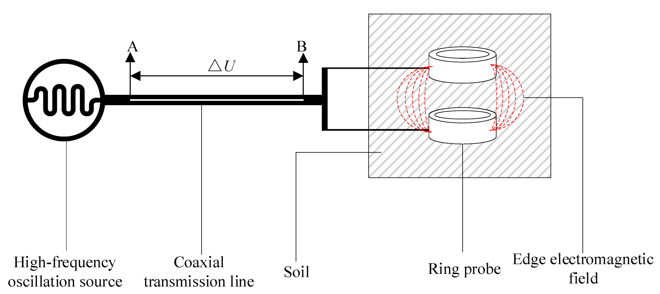
2.2. EEMFI Sensor Principle
2.3. EEMFI Sensor Hardware System
2.4. Calibration of EEMFI Sensors Based on Normalization Method
2.5. Performance Analysis of EEMFI Sensors
2.6. Sensitive Areas for Water Measurement with EEMFI Sensor
2.7. Performance Verification of EEMFI Sensor
3. Results and discussion
3.1. Calibration of EEMFI Sensors
3.2. Advantages of EEMFI Sensor Calibration Based on Normalization Method
3.3. Analysis of Static and Dynamic Characteristics of EEMFI Sensors
3.4. Analysis of Sensitive Areas for Soil Water Content Measurement
3.5. Comparative Verification of Water Measurement Performance of EEMFI Sensors
3.6. Field Experiments
3.7. Advantages and Limitations of EEMFI Sensors
4. Conclusions
Author Contributions
Funding
Institutional Review Board Statement
Informed Consent Statement
Data Availability Statement
Acknowledgments
Conflicts of Interest
References
- Eller, H.; Denoth, A. A Capacitive Soil Moisture Sensor. J. Hydrol. 1996, 185, 137–146. [Google Scholar] [CrossRef]
- Robinson, D.A.; Campbell, C.S.; Hopmans, J.W.; Hornbuckle, B.K.; Jones, S.B.; Knight, R.; Ogden, F.; Selker, J.; Wendroth, O. Soil Moisture Measurement for Ecological and Hydrological Watershed-Scale Observatories: A Review. Vadose Zone J. 2008, 7, 358–389. [Google Scholar] [CrossRef]
- Green, J.K.; Seneviratne, S.I.; Berg, A.M.; Findell, K.L.; Hagemann, S.; Lawrence, D.M.; Gentine, P. Large Influence of Soil Moisture on Long-Term Terrestrial Carbon Uptake. Nature 2019, 565, 476–479. [Google Scholar] [CrossRef] [PubMed]
- Duan, J.-R.; Li, B.; Li, S.-Z.; Li, Q. The Evaluation of Static Characteristics of Pressure Sensor Based on Conductive Rubber. In Advanced Materials, Technology and Application, Proceedings of the 2016 International Conference on Advanced Materials, Technology and Application (AMTA2016), Changsha, China 18–20 March 2016; World Scientific: Singapore, 2017; pp. 407–416. [Google Scholar]
- Placidi, P.; Gasperini, L.; Grassi, A.; Cecconi, M.; Scorzoni, A. Characterization of Low-Cost Capacitive Soil Moisture Sensors for IoT Networks. Sensors 2020, 20, 3585. [Google Scholar] [CrossRef]
- Chatterjee, S.; Desai, A.R.; Zhu, J.; Townsend, P.A.; Huang, J. Soil Moisture as an Essential Component for Delineating and Forecasting Agricultural Rather than Meteorological Drought. Remote Sens. Environ. 2022, 269, 112833. [Google Scholar] [CrossRef]
- Teixeira, J.; Correia dos Santos, R. Exploring the Applicability of Low-Cost Capacitive and Resistive Water Content Sensors on Compacted Soils. Geotech. Geol. Eng. 2021, 39, 2969–2983. [Google Scholar] [CrossRef]
- Nikolov, G.T.; Ganev, B.T.; Marinov, M.B.; Galabov, V.T. Comparative Analysis of Sensors for Soil Moisture Measurement. In Proceedings of the 2021 XXX International Scientific Conference Electronics (ET), Sozopol, Bulgaria, 15–17 September 2021; IEEE: New York, NY, USA, 2021; pp. 1–5. [Google Scholar]
- Gao, Z.; Zhu, Y.; Liu, C.; Qian, H.; Cao, W.; Ni, J. Design and Test of a Soil Profile Moisture Sensor Based on Sensitive Soil Layers. Sensors 2018, 18, 1648. [Google Scholar] [CrossRef]
- Russell, M.B.; Davis, F.E.; Bair, R.A. The Use of Tensio-Meters for Following Soil Moisture Conditions under Corn. J. Am. Soc. Agron. 1940, 32, 922–930. [Google Scholar] [CrossRef]
- Fleischhauer-Binz, E. Die Messung von Bodensaugkräften Mit Tensiometern. Planta 1949, 37, 565–594. [Google Scholar] [CrossRef]
- Jayawardane, N.S.; Meyer, W.S.; Barrs, H.D. Moisture Measurement in a Swelling Clay Soil Using Neutron Moisture Meters. Soil Res. 1984, 22, 109–117. [Google Scholar] [CrossRef]
- Votrubová, J.; Šanda, M.; Císlerová, M.; Amin, M.H.G.; Hall, L.D. The Relationships between MR Parameters and the Content of Water in Packed Samples of Two Soils. Geoderma 2000, 95, 267–282. [Google Scholar] [CrossRef]
- Kinchesh, P.; Samoilenko, A.A.; Preston, A.R.; Randall, E.W. Stray Field Nuclear Magnetic Resonance of Soil Water: Development of a New, Large Probe and Preliminary Results. J. Environ. Qual. 2002, 31, 494–499. [Google Scholar] [CrossRef] [PubMed]
- Knadel, M.; Masís-Meléndez, F.; de Jonge, L.W.; Moldrup, P.; Arthur, E.; Greve, M.H. Assessing Soil Water Repellency of a Sandy Field with Visible near Infrared Spectroscopy. J. Near Infrared Spectrosc. 2016, 24, 215–224. [Google Scholar] [CrossRef]
- Katuwal, S.; Knadel, M.; Moldrup, P.; Norgaard, T.; Greve, M.H.; de Jonge, L.W. Visible–Near-Infrared Spectroscopy Can Predict Mass Transport of Dissolved Chemicals through Intact Soil. Sci. Rep. 2018, 8, 11188. [Google Scholar] [CrossRef] [PubMed]
- Fellner-Feldegg, H. Measurement of Dielectrics in the Time Domain. J. Phys. Chem. 1969, 73, 616–623. [Google Scholar] [CrossRef]
- Topp, G.C.; St-Amour, G.; Compton, B.A.; Caron, J. Measuring Cone Resistance and Water Content with a TDR-Penetrometer Combination. In Proceedings of the 3rd Eastern Canada Soil Structure Workshop, Merrickville, ON, Canada, 21–22 August 1996; pp. 21–22. [Google Scholar]
- Topp, G.C.; Davis, J.L.; Annan, A.P. Electromagnetic Determination of Soil Water Content: Measurements in Coaxial Transmission Lines. Water Resour. Res. 1980, 16, 574–582. [Google Scholar] [CrossRef]
- Gaskin, G.J.; Miller, J.D. Measurement of Soil Water Content Using a Simplified Impedance Measuring Technique. J. Agric. Eng. Res. 1996, 63, 153–159. [Google Scholar] [CrossRef]
- Ferré, P.A.; Redman, J.D.; Rudolph, D.L.; Kachanoski, R.G. The Dependence of the Electrical Conductivity Measured by Time Domain Reflectometry on the Water Content of a Sand. Water Resour. Res. 1998, 34, 1207–1213. [Google Scholar] [CrossRef]
- Zegelin, S.J.; White, I.; Jenkins, D.R. Improved Field Probes for Soil Water Content and Electrical Conductivity Measurement Using Time Domain Reflectometry. Water Resour. Res. 1989, 25, 2367–2376. [Google Scholar] [CrossRef]
- Harlow, R.C.; Burke, E.J.; Ferré, T.P.A. Measuring Water Content in Saline Sands Using Impulse Time Domain Transmission Techniques. Vadose Zone J. 2003, 2, 433–439. [Google Scholar] [CrossRef]
- Qin, A.; Ning, D.; Liu, Z.; Duan, A. Analysis of the Accuracy of an FDR Sensor in Soil Moisture Measurement under Laboratory and Field Conditions. J. Sens. 2021, 2021, 6665829. [Google Scholar] [CrossRef]
- Miller, J.D.; Gaskin, G.J.; Anderson, H.A. From Drought to Flood: Catchment Responses Revealed Using Novel Soil Water Probes. Hydrol. Process. 1997, 11, 533–541. [Google Scholar] [CrossRef]
- Yiming, W.; Yandong, Z. Study on the Measurement of Soil Water Content Based on the Principle of Standing Wave Ratio. In Proceedings of the Beijing International Conference on Agriculture Engineering, Beijing, China, 14–17 December 1999. [Google Scholar]
- Tian, H.; Gao, C.; Zhao, Y. Combined Penetrometer and Standing Wave Ratio Probe to Measure Compactness and Moisture Content of Soils. Appl. Ecol. Environ. Res. 2019, 17, 13931–13944. [Google Scholar] [CrossRef]
- Xu, Y.; Yang, W.; Li, Z. Soil Water Sensor Based on Standing Wave Ratio Method of Design and Development. In Proceedings of the International Conference on Computer and Computing Technologies in Agriculture, Beijing, China, 16–19 September 2014; Springer: Berlin/Heidelberg, Germany, 2014; pp. 720–730. [Google Scholar]
- Zhao, Y.; Tian, H.; Han, Q.; Gu, J.; Zhao, Y. Real-Time Monitoring of Water and Ice Content in Plant Stem Based on Latent Heat Changes. Agric. For. Meteorol. 2021, 307, 108475. [Google Scholar] [CrossRef]
- Gao, C.; Tian, H.; Zhao, Y. A Novel Sensor for In Situ Detection of Freeze-Thaw Characteristics in Plants from Stem Temperature and Water Content Measurements. J. Sens. 2021, 2021, 6662769. [Google Scholar]
- Whalley, W.R.; Stafford, J. V Real-Time Sensing of Soil Water Content from Mobile Machinery: Options for Sensor Design. Comput. Electron. Agric. 1992, 7, 269–284. [Google Scholar] [CrossRef]
- Farrell, J.; Okincha, M.; Parmar, M. Sensor Calibration and Simulation. In Proceedings of the Digital Photography IV; SPIE: Bellingham, WA, USA, 2008; Volume 6817, pp. 249–257. [Google Scholar]
- Rowlandson, T.L.; Berg, A.A.; Bullock, P.R.; Ojo, E.R.; McNairn, H.; Wiseman, G.; Cosh, M.H. Evaluation of Several Calibration Procedures for a Portable Soil Moisture Sensor. J. Hydrol. 2013, 498, 335–344. [Google Scholar] [CrossRef]
- Leib, B.G.; Jabro, J.D.; Matthews, G.R. Field Evaluation and Performance Comparison of Soil Moisture Sensors. Soil Sci. 2003, 168, 396–408. [Google Scholar] [CrossRef]
- Yoder, R.E.; Johnson, D.L.; Wilkerson, J.B.; Yoder, D.C. Soilwater Sensor Performance. Appl. Eng. Agric. 1998, 14, 121–133. [Google Scholar] [CrossRef]
- Luo, C.; Wang, H.; Zhang, D.; Zhao, Z.; Li, Y.; Li, C.; Liang, K. Analytical Evaluation and Experiment of the Dynamic Characteristics of Double-Thimble-Type Fiber Bragg Grating Temperature Sensors. Micromachines 2020, 12, 16. [Google Scholar] [CrossRef]
- Doghmane, M.Y.; Lanzetta, F.; Gavignet, E. Dynamic Characterization of a Transient Surface Temperature Sensor. Procedia Eng. 2015, 120, 1245–1248. [Google Scholar] [CrossRef] [Green Version]
- González-Teruel, J.D.; Torres-Sánchez, R.; Blaya-Ros, P.J.; Toledo-Moreo, A.B.; Jiménez-Buendía, M.; Soto-Valles, F. Design and Calibration of a Low-Cost SDI-12 Soil Moisture Sensor. Sensors 2019, 19, 491. [Google Scholar] [CrossRef]
- Bircher, S.; Andreasen, M.; Vuollet, J.; Vehviläinen, J.; Rautiainen, K.; Jonard, F.; Weihermüller, L.; Zakharova, E.; Wigneron, J.-P.; Kerr, Y.H. Soil Moisture Sensor Calibration for Organic Soil Surface Layers. Geosci. Instrum. Methods Data Syst. 2016, 5, 109–125. [Google Scholar] [CrossRef]
- Vig, J.R.; Walls, F.L. A Review of Sensor Sensitivity and Stability. In Proceedings of the 2000 IEEE/EIA International Frequency Control Symposium and Exhibition (Cat. No. 00CH37052), Kansas City, MO, USA, 9 June 2000; IEEE: New York, NY, USA, 2000; pp. 30–33. [Google Scholar]
- Yu, L.; Gao, W.; Shamshiri, R.R.; Tao, S.; Ren, Y.; Zhang, Y.; Su, G. Review of Research Progress on Soil Moisture Sensor Technology. Int. J. Agric. Biol. Eng. 2021, 14, 32–42. [Google Scholar] [CrossRef]
- Hua, Y.; Zejun, T.; Zhen, X.; Dingneng, G.; Haoxing, H. Design of Soil Moisture Distribution Sensor Based on High-Frequency Capacitance. Int. J. Agric. Biol. Eng. 2016, 9, 122–129. [Google Scholar]
- Kitano, M.; Eguchi, H.; Matsui, T. Analysis of Static and Dynamic Characteristics of Humidity Sensors. Biotronics 1984, 13, 11–28. [Google Scholar]
- Kafarski, M.; Majcher, J.; Wilczek, A.; Szyplowska, A.; Lewandowski, A.; Zackiewicz, A.; Skierucha, W. Penetration Depth of a Soil Moisture Profile Probe Working in Time-Domain Transmission Mode. Sensors 2019, 19, 5485. [Google Scholar] [CrossRef]
- Mittelbach, H.; Lehner, I.; Seneviratne, S.I. Comparison of Four Soil Moisture Sensor Types under Field Conditions in Switzerland. J. Hydrol. 2012, 430, 39–49. [Google Scholar] [CrossRef]
- Walker, J.P.; Willgoose, G.R.; Kalma, J.D. In Situ Measurement of Soil Moisture: A Comparison of Techniques. J. Hydrol. 2004, 293, 85–99. [Google Scholar] [CrossRef]
- Evett, S.R.; Charlesworth, P. International Soil Moisture Sensor Comparison. Soil Water Monitoring. Irrig. Insights 2005, 1, 68–71. [Google Scholar]
- Rawls, W.J.; Brakensiek, D.L. Estimating Soil Water Retention from Soil Properties. J. Irrig. Drain. Div. 1982, 108, 166–171. [Google Scholar] [CrossRef]
- Gupta, S.; Larson, W.E. Estimating Soil Water Retention Characteristics from Particle Size Distribution, Organic Matter Percent, and Bulk Density. Water Resour. Res. 1979, 15, 1633–1635. [Google Scholar] [CrossRef]
- Geroy, I.J.; Gribb, M.M.; Marshall, H.-P.; Chandler, D.G.; Benner, S.G.; McNamara, J.P. Aspect Influences on Soil Water Retention and Storage. Hydrol. Processes 2011, 25, 3836–3842. [Google Scholar] [CrossRef]
- Eltahir, E.A.B. A Soil Moisture–Rainfall Feedback Mechanism: 1. Theory and Observations. Water Resour. Res. 1998, 34, 765–776. [Google Scholar] [CrossRef]
- Daly, E.; Porporato, A. A Review of Soil Moisture Dynamics: From Rainfall Infiltration to Ecosystem Response. Environ. Eng. Sci. 2005, 22, 9–24. [Google Scholar] [CrossRef]
- Wang, C.; Fu, B.; Zhang, L.; Xu, Z. Soil Moisture–Plant Interactions: An Ecohydrological Review. J. Soils Sediments 2019, 19, 1–9. [Google Scholar] [CrossRef]
- Scherer, T.F.; Seelig, B.; Franzen, D. Soil, Water and Plant Characteristics Important to Irrigation; NDSU: Fargo, ND, USA, 1996. [Google Scholar]
- Kong, J.; Yang, C.; Wang, J.; Wang, X.; Zuo, M.; Jin, X.; Lin, S. Deep-Stacking Network Approach by Multisource Data Mining for Hazardous Risk Identification in IoT-Based Intelligent Food Management Systems. Comput. Intell. Neurosci. 2021, 2021, 1194565. [Google Scholar] [CrossRef]
- Zheng, Y.-Y.; Kong, J.-L.; Jin, X.-B.; Wang, X.-Y.; Su, T.-L.; Zuo, M. CropDeep: The Crop Vision Dataset for Deep-Learning-Based Classification and Detection in Precision Agriculture. Sensors 2019, 19, 1058. [Google Scholar] [CrossRef]
- Jin, X.-B.; Zheng, W.-Z.; Kong, J.-L.; Wang, X.-Y.; Bai, Y.-T.; Su, T.-L.; Lin, S. Deep-Learning Forecasting Method for Electric Power Load via Attention-Based Encoder-Decoder with Bayesian Optimization. Energies 2021, 14, 1596. [Google Scholar] [CrossRef]
- Tian, H.; Zhao, Y.; Gao, C.; Xie, T.; Zheng, T.; Yu, C. Assessing the Vitality Status of Plants: Using the Correlation between Stem Water Content and External Environmental Stress. Forests 2022, 13, 1198. [Google Scholar] [CrossRef]
- Jin, X.-B.; Zheng, W.-Z.; Kong, J.-L.; Wang, X.-Y.; Zuo, M.; Zhang, Q.-C.; Lin, S. Deep-Learning Temporal Predictor via Bidirectional Self-Attentive Encoder–Decoder Framework for IOT-Based Environmental Sensing in Intelligent Greenhouse. Agriculture 2021, 11, 802. [Google Scholar] [CrossRef]
- Jin, X.-B.; Gong, W.-T.; Kong, J.-L.; Bai, Y.-T.; Su, T.-L. PFVAE: A Planar Flow-Based Variational Auto-Encoder Prediction Model for Time Series Data. Mathematics 2022, 10, 610. [Google Scholar] [CrossRef]
- Jin, X.-B.; Gong, W.-T.; Kong, J.-L.; Bai, Y.-T.; Su, T.-L. A Variational Bayesian Deep Network with Data Self-Screening Layer for Massive Time-Series Data Forecasting. Entropy 2022, 24, 335. [Google Scholar] [CrossRef] [PubMed]
- Jin, X.; Zhang, J.; Kong, J.; Su, T.; Bai, Y. A Reversible Automatic Selection Normalization (RASN) Deep Network for Predicting in the Smart Agriculture System. Agronomy 2022, 12, 591. [Google Scholar] [CrossRef]
- Kong, J.; Yang, C.; Xiao, Y.; Lin, S.; Ma, K.; Zhu, Q. A Graph-Related High-Order Neural Network Architecture via Feature Aggregation Enhancement for Identification Application of Diseases and Pests. Comput. Intell. Neurosci. 2022, 2022, 4391491. [Google Scholar] [CrossRef]
- Kong, J.; Wang, H.; Yang, C.; Jin, X.; Zuo, M.; Zhang, X. A Spatial Feature-Enhanced Attention Neural Network with High-Order Pooling Representation for Application in Pest and Disease Recognition. Agriculture 2022, 12, 500. [Google Scholar] [CrossRef]
- Kong, J.; Wang, H.; Wang, X.; Jin, X.; Fang, X.; Lin, S. Multi-Stream Hybrid Architecture Based on Cross-Level Fusion Strategy for Fine-Grained Crop Species Recognition in Precision Agriculture. Comput. Electron. Agric. 2021, 185, 106134. [Google Scholar] [CrossRef]
- Zaitouny, A.; Fragkou, A.D.; Stemler, T.; Walker, D.M.; Sun, Y.; Karakasidis, T.; Nathanail, E.; Small, M. Multiple Sensors Data Integration for Traffic Incident Detection Using the Quadrant Scan. Sensors 2022, 22, 2933. [Google Scholar] [CrossRef]
- Charakopoulos, A.K.; Katsouli, G.A.; Karakasidis, T.E. Dynamics and Causalities of Atmospheric and Oceanic Data Identified by Complex Networks and Granger Causality Analysis. Phys. A Stat. Mech. Its Appl. 2018, 495, 436–453. [Google Scholar] [CrossRef]


| Serial Number | Components and Materials | Price (USD) | Serial Number | Components and Materials | Price ($) |
|---|---|---|---|---|---|
| 1 | Bimetal ring probe | 10 | 7 | MAX485ESA | 3 |
| 2 | STM32103C8T6 | 4 | 8 | Power Control Module | 7 |
| 3 | STM8S103F2P6TR | 1 | 9 | Clock Control Module | 6 |
| 4 | CS4344 | 0.5 | 10 | PCB fabrication | 15 |
| 5 | AD8226ARZ | 3.5 | 11 | 3D Printing | 10 |
| 6 | Edge electromagnetic field detection circuit | 30 | 12 | Others (resistors, capacitors, inductors, cable wires) | 10 |
| Serial Number | Name | Production Location | Brands | Price ($) |
|---|---|---|---|---|
| 1 | TDR310W | America | Acclima | 415 |
| 2 | SDI-12 | America | Acclima | 445 |
| 3 | Soil-5MTE | China | BolunQiXiang | 370 |
| 4 | sm10 | America | Spectrum Technologies | 148 |
| 5 | TRIME-PICO-IPH | German | IMKO | 7413 |
| 6 | FT-W485 | China | FengTu | 110 |
| 7 | PICO-BT | German | IMKO | 2965 |
| 8 | HD2 | German | IMKO | 1800 |
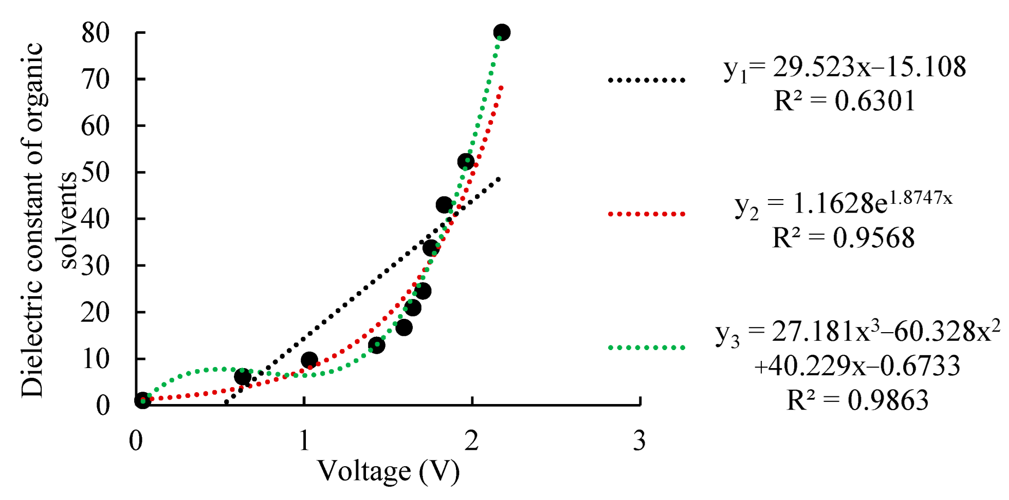
| Solution | C2H6O: H2O | CH3COOH: H2O | ||||||||
|---|---|---|---|---|---|---|---|---|---|---|
| Volume ratio | 0:1 | 1:1 | 2:1 | 5:1 | 1:0 | 4:1 | 6:1 | 10:1 | 20:1 | 1:0 |
| Dielectric constant | 80.00 | 52.25 | 43.00 | 33.75 | 24.50 | 20.92 | 16.20 | 12.86 | 9.67 | 6.15 |
| SOIL TYPE | Fitting Equation | |||
|---|---|---|---|---|
| Clay loam soil | 0.98 | 43.92 | 8.24 | |
| Loess soil | 0.99 | 48.84 | 6.22 |
| Soil Type | Soil Sample Water Content (%) | EEMFI Sensor Measurement Results (%) | Measurement Accuracy (%) |
|---|---|---|---|
| Clay loam soil | 13.72 | 13.40 | 0.32 |
| 35.80 | 37.62 | 1.82 | |
| 41.82 | 40.18 | 1.64 | |
| Loess soil | 17.88 | 16.47 | 1.41 |
| 28.97 | 26.99 | 1.98 | |
| 43.27 | 44.39 | 1.12 |
| Dynamic Characteristic | Overshoot (%) | Transition Time (s) | Delay Time (s) | Rise Time (s) | Peak Time (s) | Number of Oscillations |
|---|---|---|---|---|---|---|
| Results | 0.87 | 2.9 | 3.9 | 1.8 | 6.0 | 0 |
| Experimental Site Number | EEMFI Sensor Measurement Results (%) | Drying Method Measurement Results (%) | Absolute Error (%) |
|---|---|---|---|
| 1 | 11.7 | 13.22 | 1.52 |
| 2 | 13.9 | 12.18 | 1.72 |
| 3 | 10.2 | 11.94 | 1.74 |
| 4 | 9.8 | 10.78 | 0.98 |
| 5 | 21 | 20.3 | 0.7 |
| 6 | 12.9 | 13.26 | 0.36 |
| 7 | 18.4 | 17.92 | 0.48 |
Publisher’s Note: MDPI stays neutral with regard to jurisdictional claims in published maps and institutional affiliations. |
© 2022 by the authors. Licensee MDPI, Basel, Switzerland. This article is an open access article distributed under the terms and conditions of the Creative Commons Attribution (CC BY) license (https://creativecommons.org/licenses/by/4.0/).
Share and Cite
Tian, H.; Gao, C.; Zhang, X.; Yu, C.; Xie, T. Smart Soil Water Sensor with Soil Impedance Detected via Edge Electromagnetic Field Induction. Micromachines 2022, 13, 1427. https://doi.org/10.3390/mi13091427
Tian H, Gao C, Zhang X, Yu C, Xie T. Smart Soil Water Sensor with Soil Impedance Detected via Edge Electromagnetic Field Induction. Micromachines. 2022; 13(9):1427. https://doi.org/10.3390/mi13091427
Chicago/Turabian StyleTian, Hao, Chao Gao, Xin Zhang, Chongchong Yu, and Tao Xie. 2022. "Smart Soil Water Sensor with Soil Impedance Detected via Edge Electromagnetic Field Induction" Micromachines 13, no. 9: 1427. https://doi.org/10.3390/mi13091427