
A Monocular-Visual SLAM System with Semantic and Optical-Flow Fusion for Indoor Dynamic Environments
 , ,
, ,  , , ,
, , ,
Abstract
:1. Introduction
- (1)
- A novel monocular visual SLAM system based on ORB-SLAM2 which can achieve more accurate localization and mapping in dynamic scenes;
- (2)
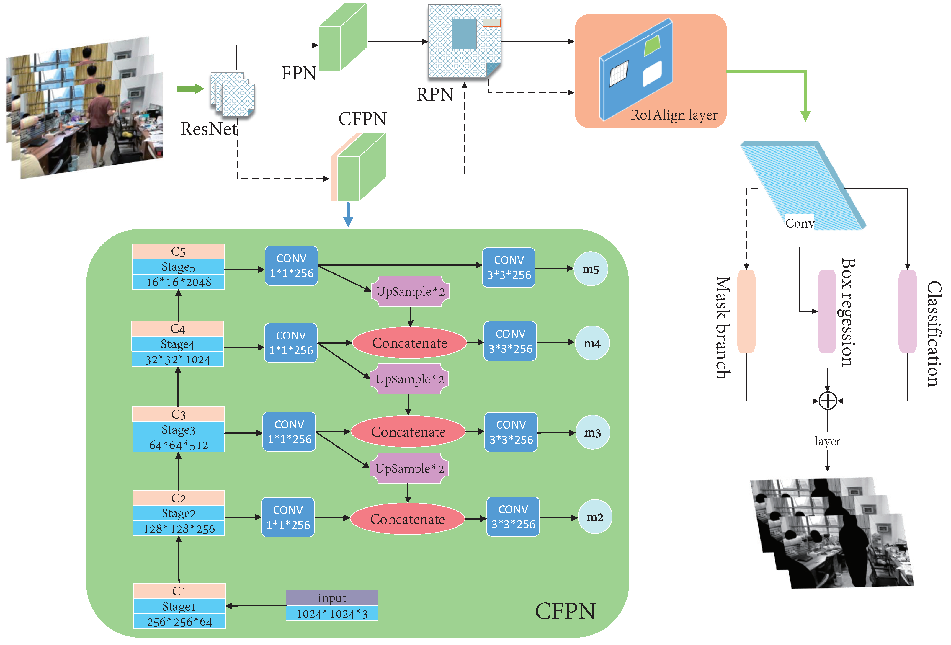
- An improved Mask R-CNN which can more accurately segment prior highly dynamic objects in indoor dynamic environments to meet the requirements of the SLAM algorithm in dynamic scenes;
- (3)
- The combination of the optical-flow method and the geometric approach, which offers a suitable and efficient dynamic-object processing strategy to remove highly dynamic objects in dynamic scenes.
2. Related Works
2.1. Visual SLAM Systems
2.2. SLAM Systems in Dynamic Scenarios
3. System Overview and Approach
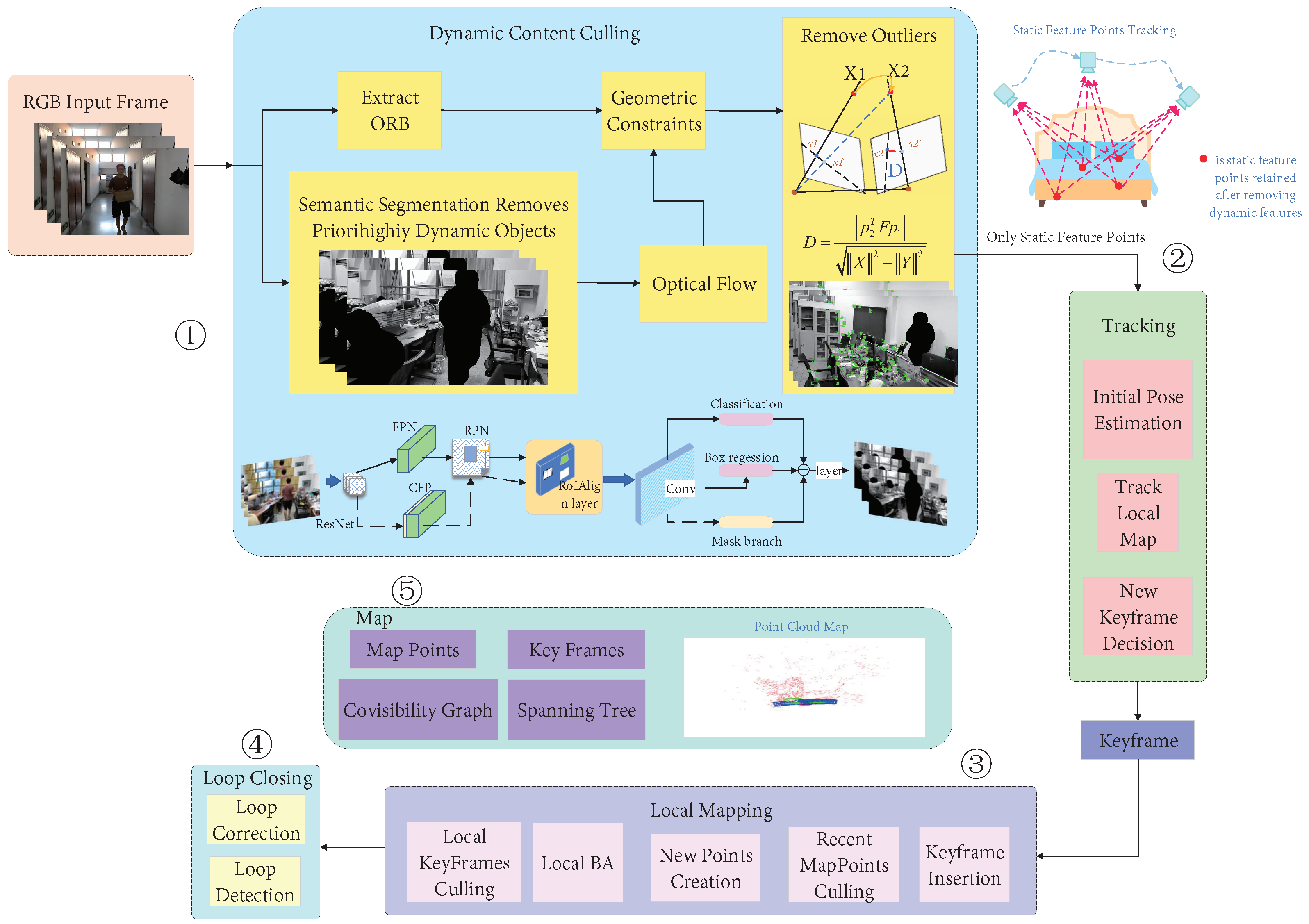
3.1. System Overview
3.2. Semantic Segmentation
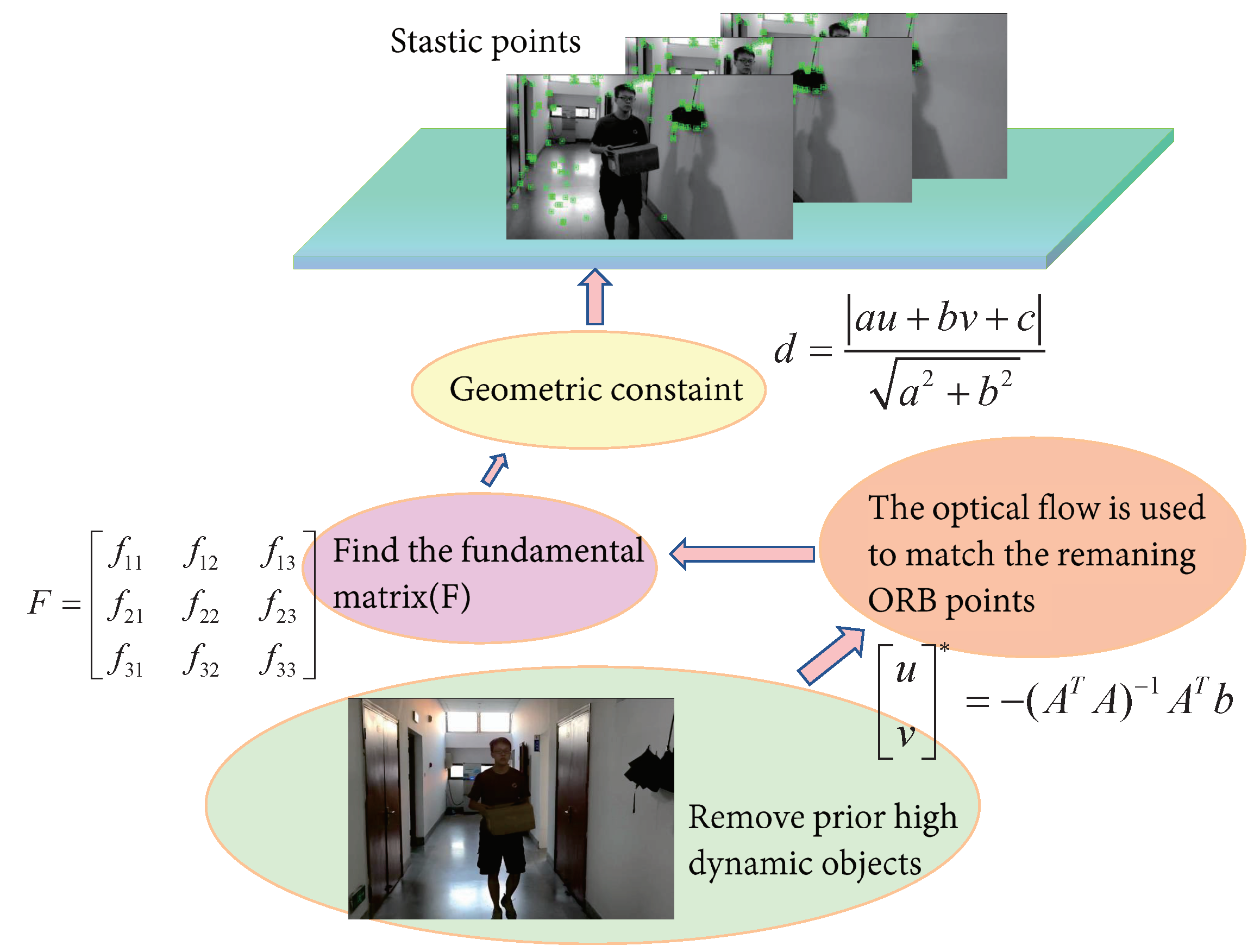
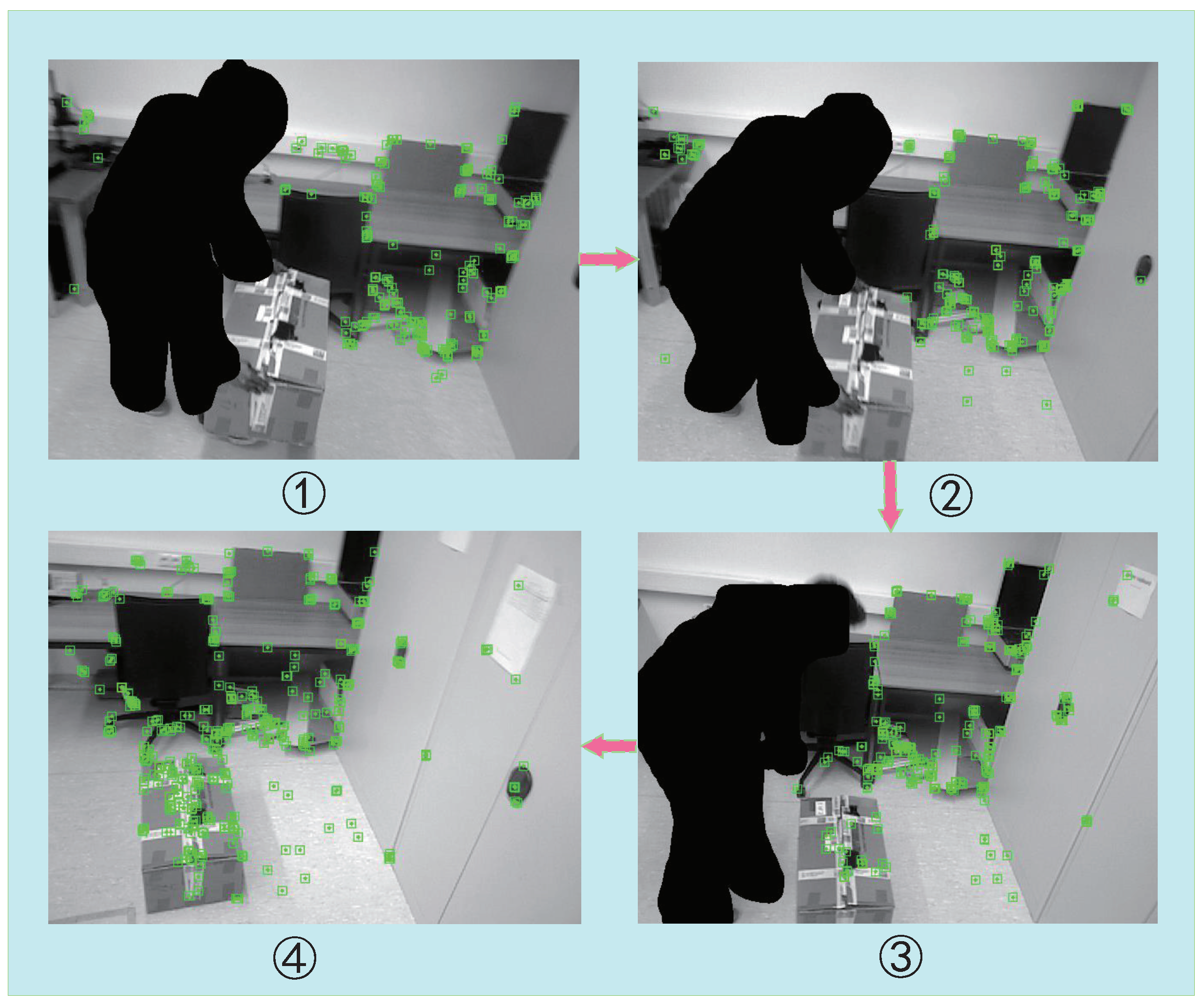
3.3. Dynamic-Object Removal
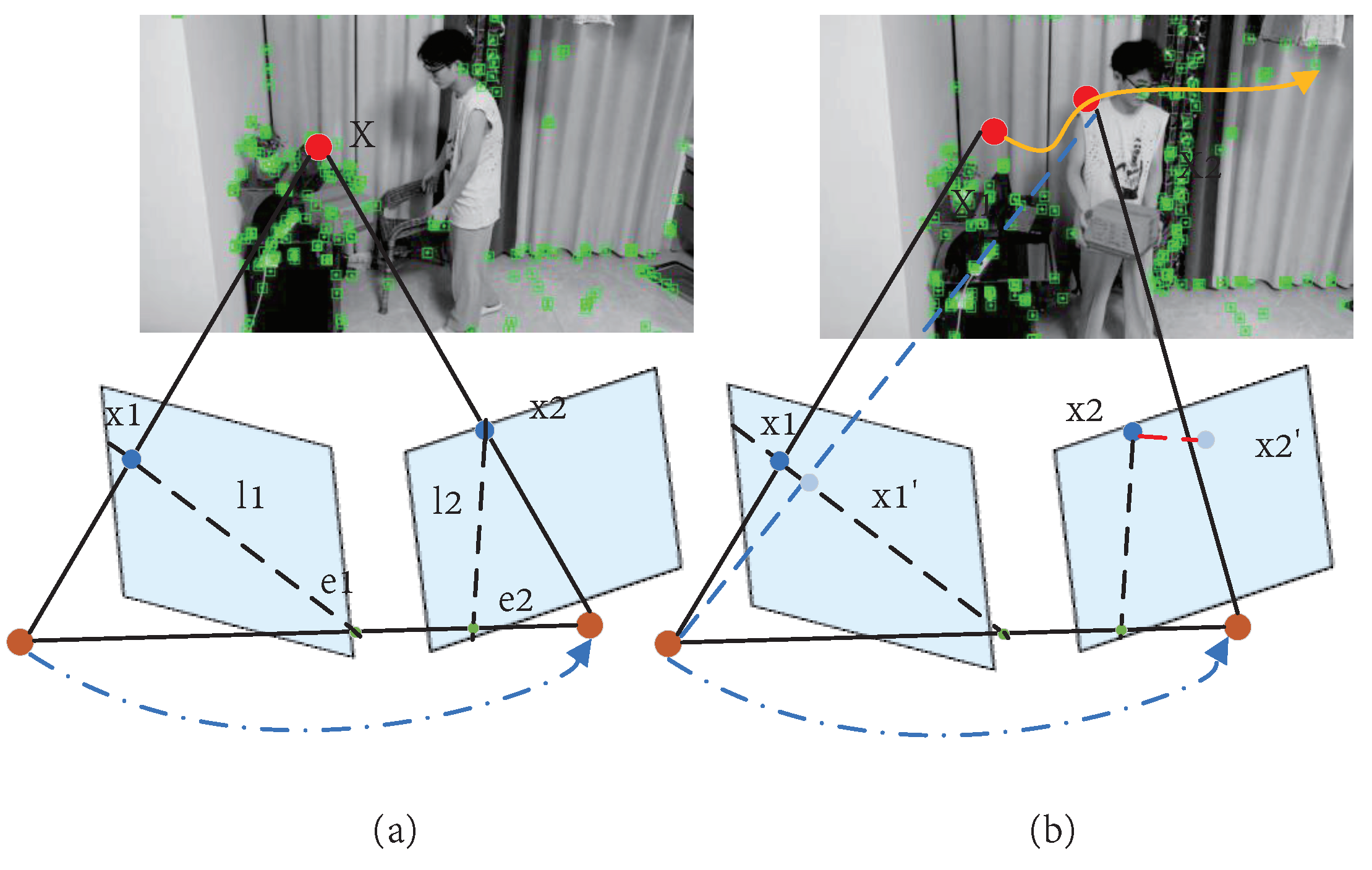
- (1)
- The optical-flow method was used to calculate the matching points of two adjacent frames to form matching point pairs;
- (2)
- A fundamental matrix for the two adjacent frames was calculated using the matching point pairs;
- (3)
- The polar line of the current frame was calculated using the base matrix;
- (4)
- The distances between all matching points and the polar line were established and any matching points whose distances exceeded the preset threshold were classified as moving points.
3.3.1. Optical-Flow Tracking
3.3.2. Geometric Constraints
4. Experimental Results
4.1. Indoor Accuracy Test on the TUM Dataset
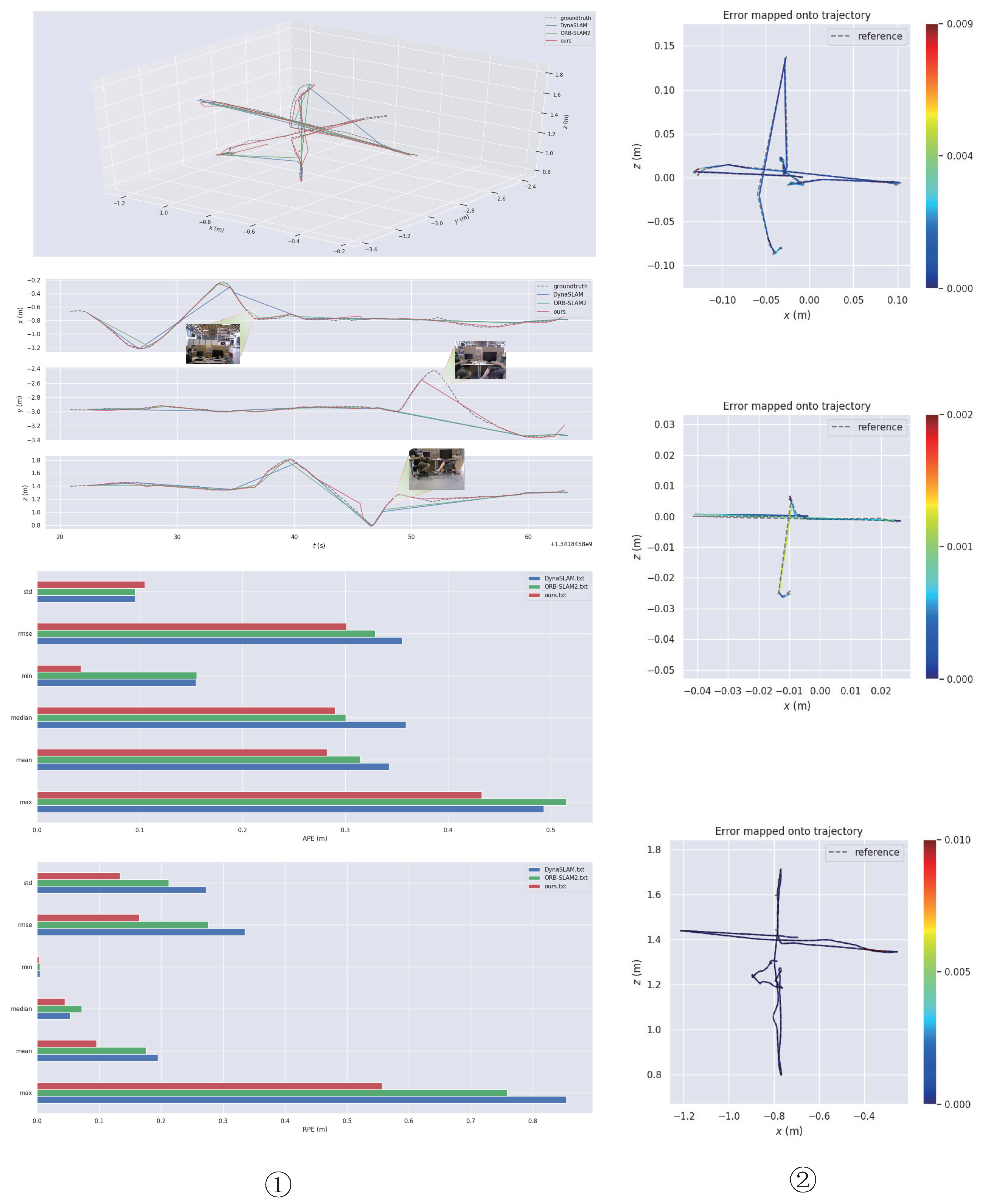
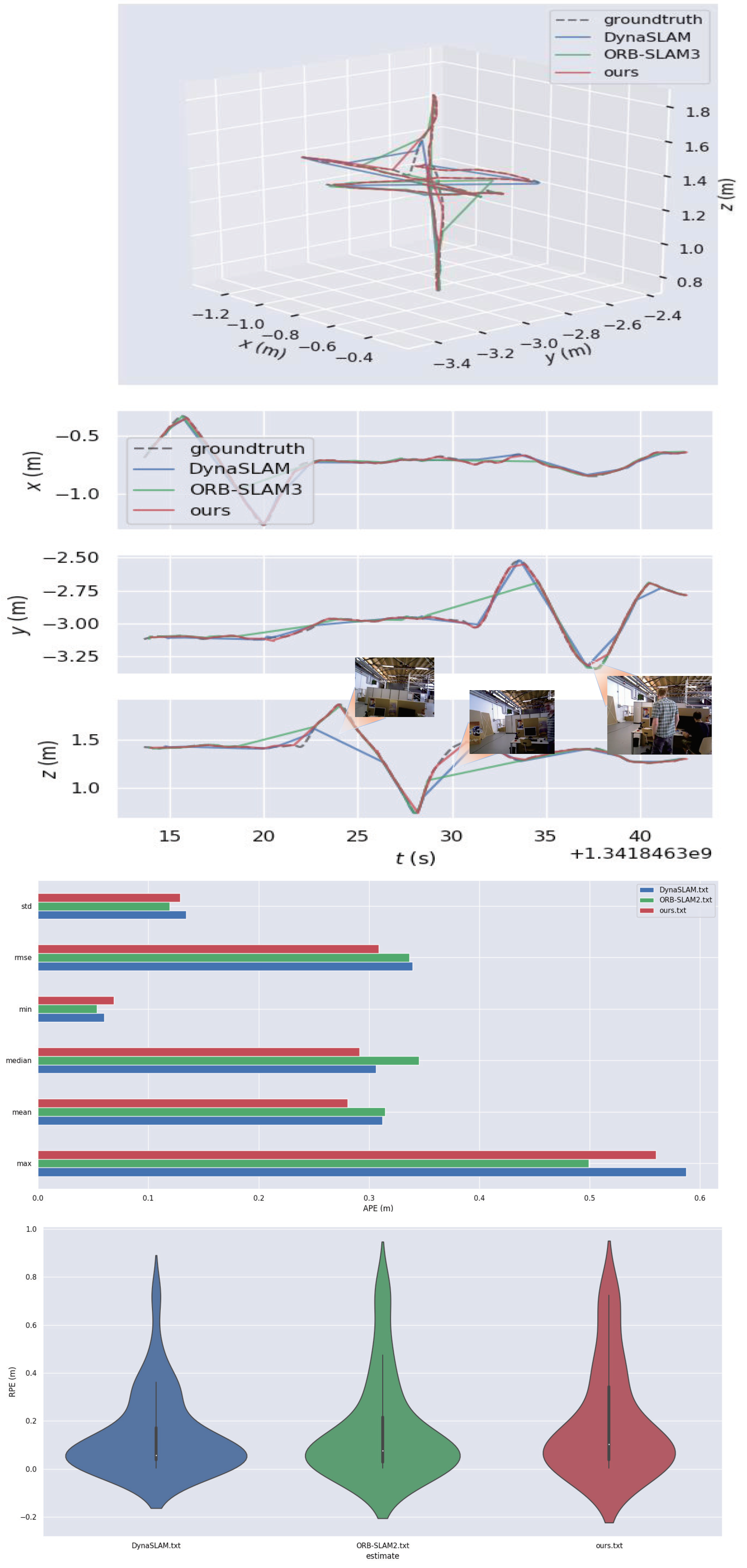
4.2. Indoor Accuracy Test on the Bonn RGB-D Dynamic Dataset

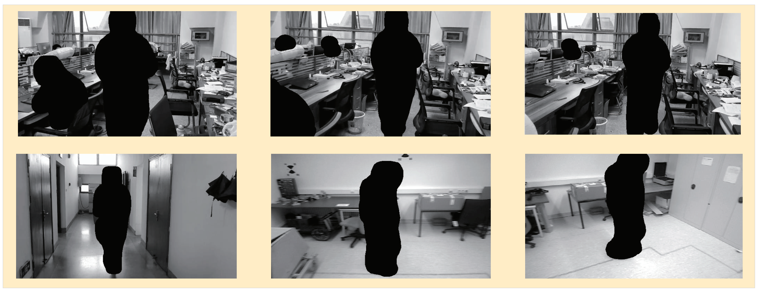
4.3. Real Environment Test


5. Discussion and Conclusions
5.1. Discussion
5.2. Conclusions
Author Contributions
Funding
Institutional Review Board Statement
Informed Consent Statement
Data Availability Statement
Acknowledgments
Conflicts of Interest
Abbreviations
| SLAM | Simultaneous Localization And Mapping |
| SSD | Single Shot Detection |
| VSLAM | Visual Simultaneous Localization And Mapping |
| FPN | Feature Pyramid Network |
| RPN | Region Proposal Network |
| CFPN | Cross-layer Feature Pyramid Network |
| APE | Absolute Pose Error |
| RPE | Relative Pose Error |
| RMSE | Root Mean Square Error |
| StD | Mean and Standard Deviation |
References
- Taheri, H.; Xia, Z.C. SLAM: Definition and evolution. Eng. Appl. Artif. Intell. 2021, 97, 104032. [Google Scholar] [CrossRef]
- Chen, Q.; Yao, L.; Xu, L.; Yang, Y.; Xu, T.; Yang, Y.; Liu, Y. Horticultural Image Feature Matching Algorithm Based on Improved ORB and LK Optical Flow. Remote Sens. 2022, 14, 4465. [Google Scholar] [CrossRef]
- Younes, G.; Asmar, D.; Shammas, E.; Zelek, J. Keyframe-based monocular SLAM: Design, survey, and future directions. Robot. Auton. Syst. 2017, 98, 67–88. [Google Scholar] [CrossRef] [Green Version]
- Davison, A.J.; Reid, I.D.; Molton, N.D.; Stasse, O. MonoSLAM: Real-Time Single Camera SLAM. IEEE Trans. Pattern Anal. Mach. Intell. 2007, 29, 1052–1067. [Google Scholar] [CrossRef] [Green Version]
- Mur-Artal, R.; Tardos, J.D. ORB-SLAM2: An Open-Source SLAM System for Monocular, Stereo, and RGB-D Cameras. IEEE Trans. Robot. 2017, 33, 1255–1262. [Google Scholar] [CrossRef] [Green Version]
- Qin, T.; Li, P.; Shen, S. VINS-Mono: A Robust and Versatile Monocular Visual-Inertial State Estimator. IEEE Trans. Robot. 2018, 34, 1004–1020. [Google Scholar] [CrossRef] [Green Version]
- Wang, Z.; Zhang, Q.; Li, J.; Zhang, S.; Liu, J. A Computationally Efficient Semantic SLAM Solution for Dynamic Scenes. Remote Sens. 2021, 11, 1363. [Google Scholar] [CrossRef] [Green Version]
- Sun, L.; Wei, J.; Su, S.; Wu, P. SOLO-SLAM: A Parallel Semantic SLAM Algorithm for Dynamic Scenes. Sensors 2022, 22, 6977. [Google Scholar] [CrossRef]
- Liu, Y.; Zhou, Z. Optical Flow-Based Stereo Visual Odometry With Dynamic Object Detection. IEEE Trans. Comput. Soc. Syst. 2022, 2, 1–13. [Google Scholar] [CrossRef]
- Liu, L.; Guo, J.; Zhang, R. YKP-SLAM: A Visual SLAM Based on Static Probability Update Strategy for Dynamic Environments. Electronics 2022, 11, 2872. [Google Scholar] [CrossRef]
- Chen, W.; Shang, G.; Ji, A.; Zhou, C.; Wang, X.; Xu, C.; Li, Z.; Hu, K. An Overview on Visual SLAM: From Tradition to Semantic. Remote Sens. 2022, 14, 3010. [Google Scholar] [CrossRef]
- Song, S.; Lim, H.; Lee, A.J.; Myung, H. DynaVINS: A Visual-Inertial SLAM for Dynamic Environments. IEEE Robot. Autom. Lett. 2022, 7, 11523–11530. [Google Scholar] [CrossRef]
- Gökcen, B.; Uslu, E. Object Aware RGBD SLAM in Dynamic Environments. In Proceedings of the 2022 International Conference on INnovations in Intelligent SysTems and Applications (INISTA), Biarritz, France, 8–12 August 2022; pp. 1–6. [Google Scholar]
- Klein, G.; Murray, D. Parallel Tracking and Mapping for Small AR Workspaces. In Proceedings of the IEEE & ACM International Symposium on Mixed & Augmented Reality, Nara, Japan, 13–16 November 2007; pp. 225–234. [Google Scholar]
- Engel, J.; Schöps, T.; Cremers, D. LSD-SLAM: Large-Scale Direct Monocular SLAM. In Proceedings of the Computer Vision—ECCV 2014, Zurich, Switzerland, 6–12 September 2014; pp. 834–849. [Google Scholar]
- Forster, C.; Pizzoli, M.; Scaramuzza, D. SVO: Fast semi-direct monocular visual odometry. In Proceedings of the 2014 IEEE International Conference on Robotics and Automation (ICRA), Hong Kong, China, 31 May–7 June 2014; pp. 15–22. [Google Scholar]
- Bavle, H.; Sánchez-López, J.L.; Schmidt, E.F.; Voos, H.J.A. From SLAM to Situational Awareness: Challenges and Survey. arXiv 2021, arXiv:2110.00273. [Google Scholar]
- Li, G.H.; Chen, S.L. Visual Slam in Dynamic Scenes Based on Object Tracking and Static Points Detection. J. Intell. Robot. Syst. 2022, 104, 33. [Google Scholar] [CrossRef]
- Mur-Artal, R.; Montiel, J.M.M.; Tardos, J.D. ORB-SLAM: A Versatile and Accurate Monocular SLAM System. IEEE Trans. Robot. 2015, 31, 1147–1163. [Google Scholar] [CrossRef] [Green Version]
- Campos, C.; Elvira, R.; Rodriguez, J.J.G.; Montiel, J.M.M.; Tardos, J.D. ORB-SLAM3: An Accurate Open-Source Library for Visual, Visual-Inertial, and Multimap SLAM. IEEE Trans. Robot. 2021, 34, 1874–1890. [Google Scholar] [CrossRef]
- Macario Barros, A.; Michel, M.; Moline, Y.; Corre, G.; Carrel, F. A Comprehensive Survey of Visual SLAM Algorithms. Robotics 2022, 11, 24. [Google Scholar] [CrossRef]
- Wang, K.; Ma, S.; Chen, J.L.; Ren, F.; Lu, J.B. Approaches, Challenges, and Applications for Deep Visual Odometry: Toward Complicated and Emerging Areas. IEEE Trans. Cogn. Dev. Syst. 2022, 11, 35–49. [Google Scholar] [CrossRef]
- Durrant-Whyte, H.; Bailey, T. Simultaneous localization and mapping: Part I. IEEE Robot. Autom. Mag. 2006, 13, 99–110. [Google Scholar] [CrossRef] [Green Version]
- Karam, S.; Nex, F.; Chidura, B.T.; Kerle, N. Microdrone-Based Indoor Mapping with Graph SLAM. Drones 2022, 6, 352. [Google Scholar] [CrossRef]
- Michael, E.; Summers, T.H.; Wood, T.A.; Manzie, C.; Shames, I. Probabilistic Data Association for Semantic SLAM at Scale. arXiv 2022, arXiv:2202.12802. [Google Scholar]
- Liu, Y.; Zhao, C.; Ren, M. An Enhanced Hybrid Visual–Inertial Odometry System for Indoor Mobile Robot. Sensors 2022, 22, 2930. [Google Scholar] [PubMed]
- Pei, R.; Fu, W.; Yao, K.; Zheng, T.; Ding, S.; Zhang, H.; Zhang, Y. Real-Time Multi-Focus Biomedical Microscopic Image Fusion Based on m-SegNet. EEE Photonics J. 2021, 13, 8600118. [Google Scholar] [CrossRef]
- Sun, X.; Xie, Y.; Jiang, L.; Cao, Y.; Liu, B. DMA-Net: DeepLab With Multi-Scale Attention for Pavement Crack Segmentation. IEEE Trans. Intell. Transp. Syst. 2022, 23, 18392–18403. [Google Scholar] [CrossRef]
- Hu, Z.; Zhao, J.; Luo, Y.; Ou, J. Semantic SLAM Based on Improved DeepLabv3+ in Dynamic Scenarios. IEEE Access 2022, 10, 21160–21168. [Google Scholar] [CrossRef]
- Qian, Z.; Patath, K.; Fu, J.; Xiao, J. Semantic SLAM with Autonomous Object-Level Data Association. In Proceedings of the 2021 IEEE International Conference on Robotics and Automation (ICRA), Xi’an, China, 30 May–5 June 2021; pp. 11203–11209. [Google Scholar]
- Zhang, X.; Zhang, R.; Wang, X. Visual SLAM Mapping Based on YOLOv5 in Dynamic Scenes. Appl. Sci. 2022, 12, 11548. [Google Scholar] [CrossRef]
- Zhong, F.; Wang, S.; Zhang, Z.; Chen, C.; Wang, Y. Detect-SLAM: Making Object Detection and SLAM Mutually Beneficial. In Proceedings of the 2018 IEEE Winter Conference on Applications of Computer Vision (WACV), Lake Tahoe, NV, USA, 12–15 March 2018; pp. 1001–1010. [Google Scholar]
- Bescos, B.; Fácil, J.M.; Civera, J.; Neira, J. DynaSLAM: Tracking, Mapping, and Inpainting in Dynamic Scenes. IEEE Robot. Autom. Lett. 2018, 3, 4076–4083. [Google Scholar] [CrossRef] [Green Version]
- He, K.; Gkioxari, G.; Dollár, P.; Girshick, R.B. Mask R-CNN. In Proceedings of the IEEE International Conference on Computer Vision, Venice, Italy, 22–29 October 2017; pp. 2980–2988. [Google Scholar]
- Yu, C.; Liu, Z.; Liu, X.J.; Xie, F.; Yang, Y.; Wei, Q.; Fei, Q. DS-SLAM: A Semantic Visual SLAM towards Dynamic Environments. In Proceedings of the 2018 IEEE/RSJ International Conference on Intelligent Robots and Systems (IROS), Madrid, Spain, 1–5 October 2018; pp. 1168–1174. [Google Scholar]
- Cui, L.; Ma, C. SOF-SLAM: A Semantic Visual SLAM for Dynamic Environments. IEEE Access 2019, 7, 166528–166539. [Google Scholar] [CrossRef]
- Zhang, S.; Wang, Z.; Zhu, Q. Research on Loop Closure Detection Method Based on ResNet. In Proceedings of the 2021 Asia-Pacific Conference on Communications Technology and Computer Science (ACCTCS), Shenyang, China, 22–24 January 2021; pp. 246–249. [Google Scholar]
- Zhou, X.; Zhang, L. SA-FPN: An effective feature pyramid network for crowded human detection. Appl. Intell. 2022, 52, 12556–12568. [Google Scholar] [CrossRef]
- Wen, K.; Chu, J.; Chen, J.; Chen, Y.; Cai, J. M-O SiamRPN with Weight Adaptive Joint MIoU for UAV Visual Localization. Remote Sens. 2022, 14, 4467. [Google Scholar] [CrossRef]
- Zhao, K.; Wang, Y.; Zhu, Q.; Zuo, Y. Intelligent Detection of Parcels Based on Improved Faster R-CNN. Appl. Sci. 2022, 12, 7158. [Google Scholar] [CrossRef]
- Mubarak, A.S.; Vubangsi, M.; Al-Turjman, F.; Ameen, Z.S.; Mahfudh, A.S.; Alturjman, S. Computer Vision Based Drone Detection Using Mask R-CNN. In Proceedings of the 2022 International Conference on Artificial Intelligence in Everything (AIE), Kitakyushu, Japan, 2–4 August 2022; pp. 540–543. [Google Scholar]
- Liu, Y.; Miura, J. RDMO-SLAM: Real-Time Visual SLAM for Dynamic Environments Using Semantic Label Prediction With Optical Flow. IEEE Access 2021, 9, 106981–106997. [Google Scholar] [CrossRef]
- Goyal, A.; Mousavian, A.; Paxton, C.; Chao, Y.W.; Okorn, B.; Deng, J.; Fox, D. IFOR: Iterative Flow Minimization for Robotic Object Rearrangement. In Proceedings of the 2022 IEEE/CVF Conference on Computer Vision and Pattern Recognition (CVPR), New Orleans, LA, USA, 18–24 June 2022; pp. 14767–14777. [Google Scholar]
- Liu, S.; Wang, X.; Chen, X.; Hou, X.; Zhang, X.; Jiang, T.; Zhang, X. Simulation and experiment of tomato pollen particles release and motion characteristics based on optical flow target tracking method. Comput. Electron. Agric. 2022, 198, 107106. [Google Scholar] [CrossRef]
- Jiang, J.; Chen, X.; Dai, W.; Gao, Z.; Zhang, Y. Thermal-Inertial SLAM for the Environments With Challenging Illumination. IEEE Robot. Autom. Lett. 2022, 7, 8767–8774. [Google Scholar] [CrossRef]
- Giubilato, R.; Stürzl, W.; Wedler, A.; Triebel, R. Challenges of SLAM in Extremely Unstructured Environments: The DLR Planetary Stereo, Solid-State LiDAR, Inertial Dataset. IEEE Robot. Autom. Lett. 2022, 2022 7, 8721–8728. [Google Scholar] [CrossRef]
- Dai, W.; Zhang, Y.; Li, P.; Fang, Z.; Scherer, S.; Intelligence, M. RGB-D SLAM in Dynamic Environments Using Point Correlations. IEEE Trans. Cogn. Dev. Syst. 2020, 44, 373–389. [Google Scholar] [CrossRef]
- Li, Q.; Wang, X.; Wu, T.; Yang, H. Point-line feature fusion based field real-time RGB-D SLAM. Comput. Graph. 2022, 107, 10–19. [Google Scholar] [CrossRef]
- Yan, L.; Hu, X.; Zhao, L.; Chen, Y.; Wei, P.; Xie, H. DGS-SLAM: A Fast and Robust RGBD SLAM in Dynamic Environments Combined by Geometric and Semantic Information. Remote Sens. 2022, 14, 795. [Google Scholar] [CrossRef]


| Method | APE (m) | RPE (m) | ||||||
|---|---|---|---|---|---|---|---|---|
| Mean | Median | RMSE | StD | Mean | Median | RMSE | StD | |
| ORB-SLAM2 | 0.3148 | 0.3004 | 0.329 | 0.096 | 0.1761 | 0.0713 | 0.2757 | 0.2122 |
| DynaSLAM | 0.3425 | 0.3589 | 0.3555 | 0.0953 | 0.1948 | 0.0531 | 0.3348 | 0.2723 |
| Ours | 0.2785 | 0.2869 | 0.2973 | 0.1041 | 0.1011 | 0.0506 | 0.1679 | 0.1341 |
| Method | APE (m) | RPE (m) | ||||||
|---|---|---|---|---|---|---|---|---|
| Mean | Median | RMSE | StD | Mean | Median | RMSE | StD | |
| ORB-SLAM2 | 0.3147 | 0.3452 | 0.3375 | 0.1191 | 0.1589 | 0.0753 | 0.2572 | 0.2023 |
| DynaSLAM | 0.3119 | 0.3065 | 0.3396 | 0.1341 | 0.1403 | 0.0577 | 0.2162 | 0.1644 |
| Ours | 0.2805 | 0.2913 | 0.3087 | 0.1288 | 0.1017 | 0.1022 | 0.2911 | 0.2909 |
| Tracking Time (s) | TUM Sequence | |||||
|---|---|---|---|---|---|---|
| sitting_xyz | walking_xyz | |||||
| ORB-SLAM2 | Ours | DynaSLAM | ORB-SLAM2 | Ours | DynaSLAM | |
| Median | 0.01843 | 4.23753 | 4.54982 | 0.01861 | 3.99734 | 4.23104 |
| Mean | 0.01942 | 4.20628 | 4.51254 | 0.02148 | 4.01317 | 4.30717 |
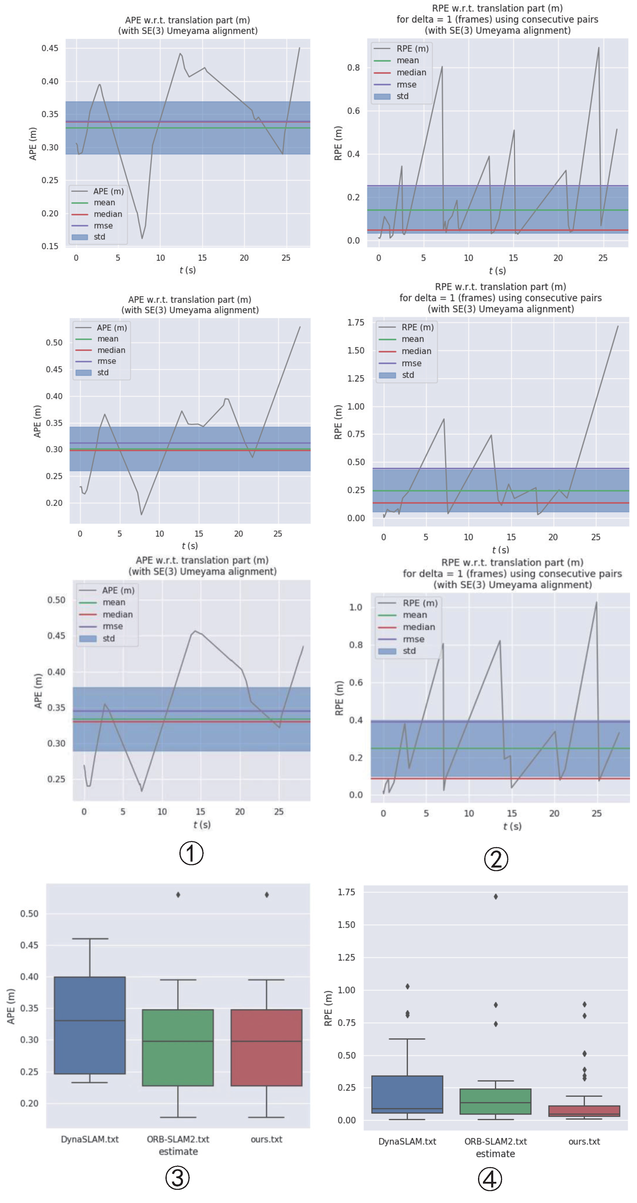
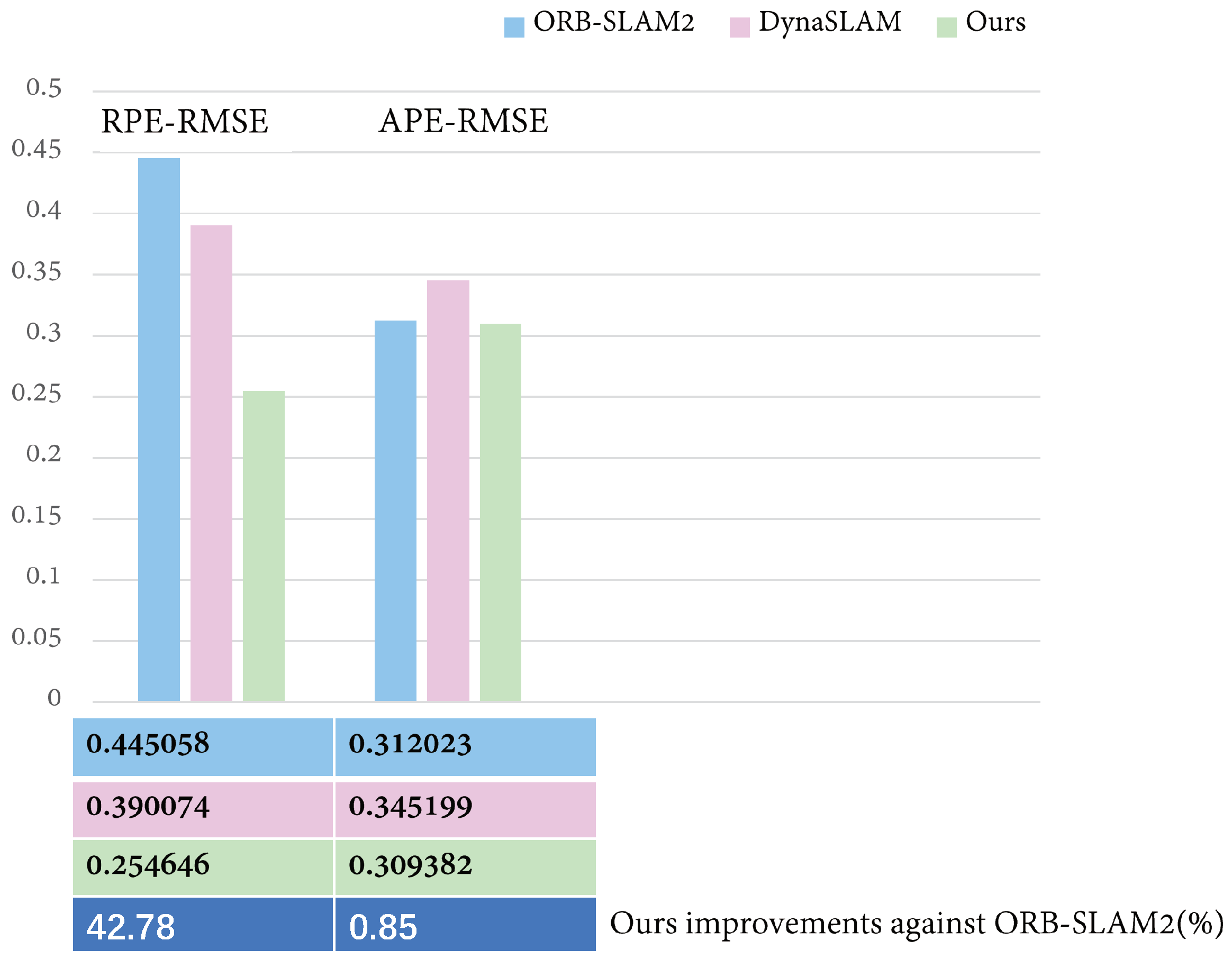
| rgbd_bonn_moving_ nonobstructing_box2 | Ours | ORB-SLAM2 | DynaSLAM | |
|---|---|---|---|---|
| RPE (m) | Mean | 0.141 | 0.243 | 0.249 |
| Median | 0.048 | 0.135 | 0.088 | |
| RMSE | 0.254 | 0.445 | 0.39 | |
| SSD | 2.464 | 4.753 | 3.195 | |
| StD | 0.212 | 0.372 | 0.3 | |
| APE (m) | Mean | 0.33 | 0.301 | 0.334 |
| Median | 0.338 | 0.298 | 0.33 | |
| RMSE | 0.309 | 0.312 | 0.345 | |
| SSD | 4.492 | 2.439 | 2.622 | |
| StD | 0.08 | 0.082 | 0.088 | |
| Median Tracking Time (s) | 4.20007 | 0.01697 | 4.42606 | |
| Mean Tracking Time (s) | 4.19947 | 0.01764 | 4.47998 | |
Publisher’s Note: MDPI stays neutral with regard to jurisdictional claims in published maps and institutional affiliations. |
© 2022 by the authors. Licensee MDPI, Basel, Switzerland. This article is an open access article distributed under the terms and conditions of the Creative Commons Attribution (CC BY) license (https://creativecommons.org/licenses/by/4.0/).
Share and Cite
Chen, W.; Shang, G.; Hu, K.; Zhou, C.; Wang, X.; Fang, G.; Ji, A. A Monocular-Visual SLAM System with Semantic and Optical-Flow Fusion for Indoor Dynamic Environments. Micromachines 2022, 13, 2006. https://doi.org/10.3390/mi13112006
Chen W, Shang G, Hu K, Zhou C, Wang X, Fang G, Ji A. A Monocular-Visual SLAM System with Semantic and Optical-Flow Fusion for Indoor Dynamic Environments. Micromachines. 2022; 13(11):2006. https://doi.org/10.3390/mi13112006
Chicago/Turabian StyleChen, Weifeng, Guangtao Shang, Kai Hu, Chengjun Zhou, Xiyang Wang, Guisheng Fang, and Aihong Ji. 2022. "A Monocular-Visual SLAM System with Semantic and Optical-Flow Fusion for Indoor Dynamic Environments" Micromachines 13, no. 11: 2006. https://doi.org/10.3390/mi13112006