
Steric and Slippage Effects on Mass Transport by Using an Oscillatory Electroosmotic Flow of Power-Law Fluids


Abstract
:1. Introduction
2. Problem Formulation
2.1. Electrical Field: Steric Effects
2.2. Velocity Field
2.3. Concentration Field
2.4. Mass Transport Rate
3. Numerical Scheme
3.1. Electric Potential Field
3.2. Velocity Field
3.3. Concentration Field and Mass Transport Rate
4. Results and Discussion
5. Conclusions
- In shear-thinning fluids, the steric effect under hydrophobic conditions has a noticeable impact on the rheology of the fluid, causing higher values in the dynamic viscosity, , compared with the absence of finite-size ions. In shear-thickening fluids, since steric effects reduce the oscillatory electroosmotic body force up to three orders of magnitude compared with no steric case, the dynamic viscosity decreases near the microchannel wall.
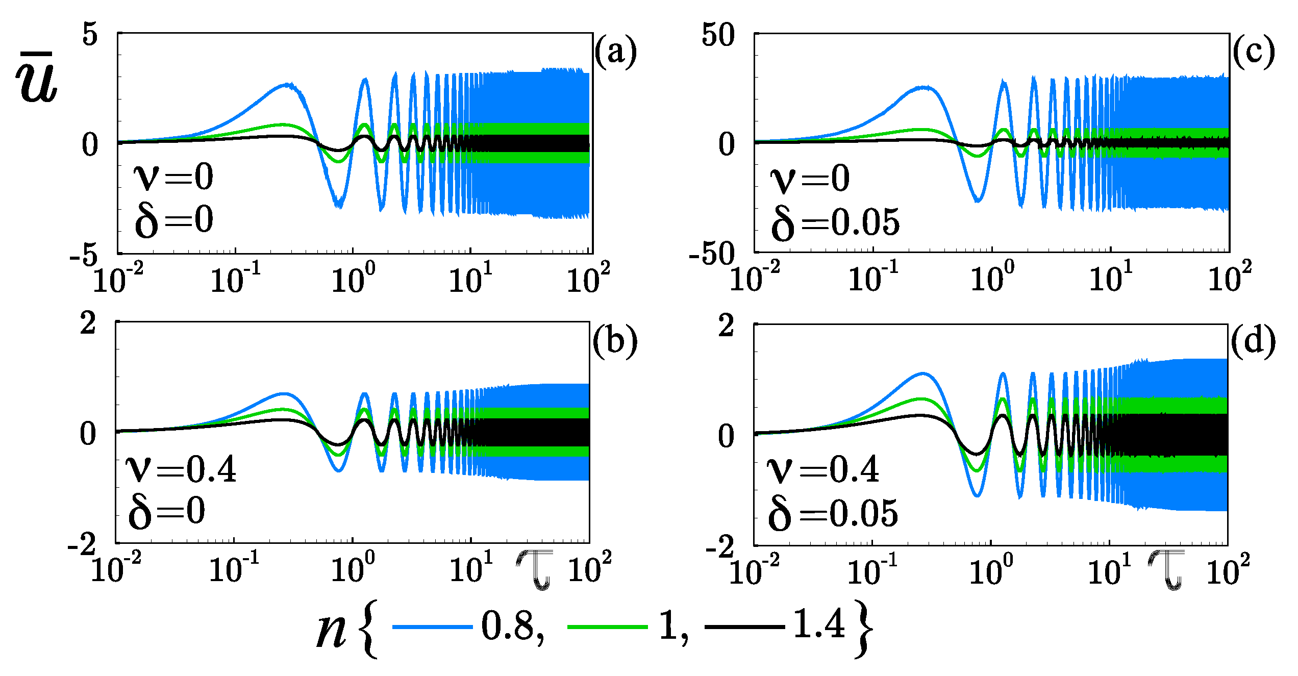
- Finite-size ions reduce oscillatory electroosmotic body force by preventing EDL from being highly concentrated. As a result, steric effects result in a decrease in velocity in shear-thinning fluids up to one order of magnitude compared with no steric case, with . However, in shear-thickening fluids, the steric effects are negligible on the velocity when .
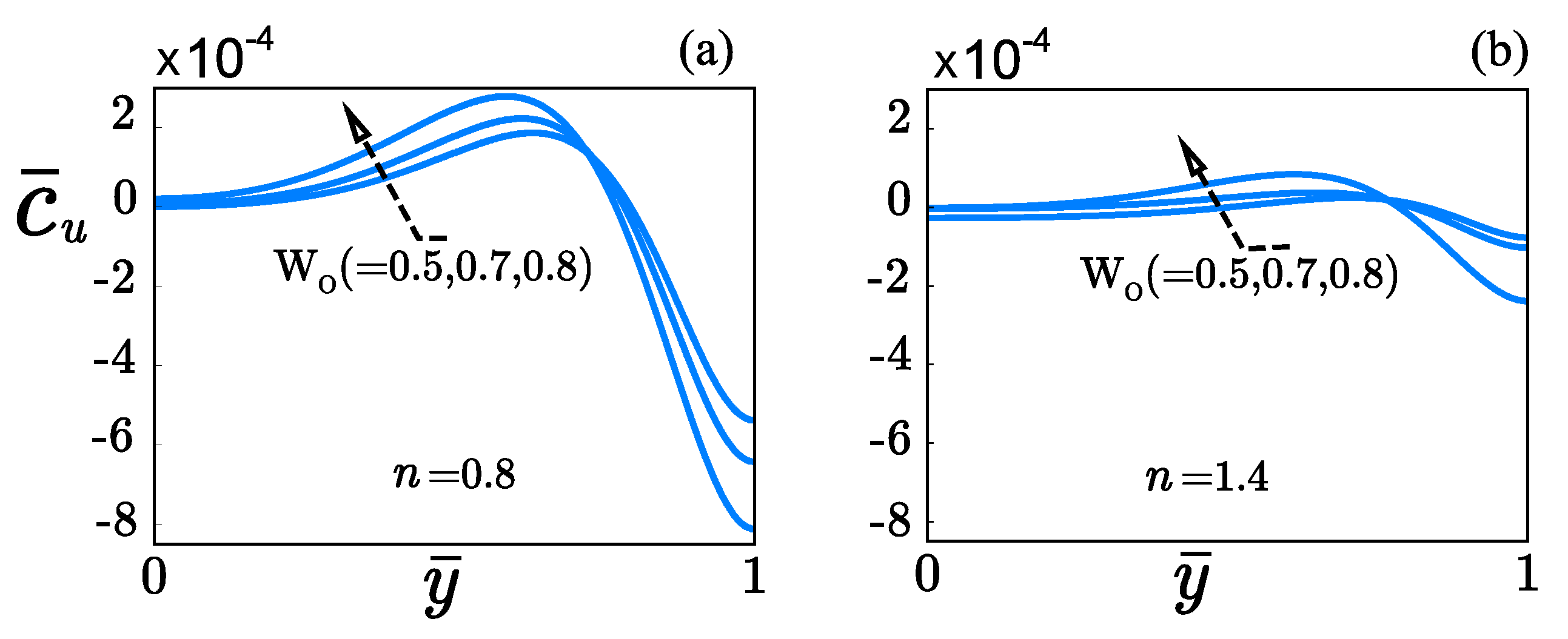
- The suggested values of , and promote the best conditions for the mass transport for any number values. A value of with increases the value of in about 90 % compared with no steric effect. In a similar way, in about 20 % the value of was increased with .
- The steric effect enhances the mass transport in fast and slow diffusers when increases by using or high zeta potentials (). However, at high zeta potentials (), increases up to one order of magnitude compared with that obtained with . Additionally, steric effect promotes that slow diffusers () can travel faster than fast diffusers () at , as shown in Figure 9 (black lines). The opposite behavior occurs in the absence of steric effects.
- A wide variety of different physical and chemical phenomena could also be included in the model to examine their effects on mass transport with non-Newtonian fluids. Possibilities include the depletion of macromolecules near the microchannel walls, the presence of a reversible reaction or mass exchange between the microchannel wall and the fluid. In physiological systems, which can be significantly more important viscoelastic effects than higher purity for typical aqueous solutions, could be considered.
Author Contributions
Funding
Acknowledgments
Conflicts of Interest
Abbreviations
| a | Ion size, m |
| c | Concentration field of the solute, mol m−3 |
| Molar ion concentration of the electrolyte solution, mol m−3 | |
| Fixed concentration values at the ends of the microchannel, mol m−3 | |
| Convective species concentration, mol m−3 | |
| Dimensionless convective species concentration | |
| D | Diffusion coefficient, m2 s−1 |
| Rate of strain tensor | |
| e | Electron charge, C |
| External electric field, Vm−1 | |
| Intensity of the applied electric field, Vm−1 | |
| h | Microchannel Half-Height, m |
| Convective flux density, mol m2 s−1 | |
| Diffusive flux density x, mol m2 s−1 | |
| Total flux density, mol m2 s−1 | |
| Boltzmann constant, J K−1 | |
| L | Microchannel length, m |
| m | Fluid consistency index, Pa sn |
| Dimensionless consistency index | |
| n | Power-law index |
| Unit vector normal to the microchannel surface | |
| Ionic concentration, m−3 | |
| Diffusive Péclet number | |
| Flow rate, mol m−2 s−1 | |
| Dimensionless flow rate | |
| Schmidt number | |
| t | Time, s |
| Periodic time, s | |
| T | Absolute temperature, K |
| u | Longitudinal velocity component, m s−1 |
| Fluid velocity at the microchannel wall, m s−1 | |
| Helmholtz-Smoluchowsky velocity | |
| Dimensionless longitudinal velocity component | |
| Womersley number | |
| Space coordinates, m | |
| Dimensionless space coordinates | |
| z | valency of both the ions |
| Aspect ratio | |
| Strain rate | |
| Tidal displacement, m | |
| Dimensionless tidal displacement | |
| Dimensionless slip lenght | |
| Permittivity of the solution, C V−1 m−1 | |
| Zeta potential, V | |
| Apparent viscosity of the fluid, Pa s | |
| Debye length, m | |
| Relation between the wall potential and the thermal potential | |
| Ratio of the microchannel height to the Debye length | |
| Navier length, m | |
| Viscosity of a Newtonian fluid, Pa s | |
| Bulk volume fraction of ions | |
| Kinematic viscosity, m2 s−1 | |
| Fluid density, kg m−3 | |
| Electric charge density, C m−3 | |
| Dimensionless time | |
| Dimensionless periodic time | |
| Unidirectional shear stress | |
| Total electric potential, V | |
| External electric potential, V | |
| Electric potential, V | |
| Angular frequency, rad s−1 | |
| i | Nodal position in coordinate |
| j | Nodal position in coordinate |
| l | Nodal position in time |
| Matrix transpose | |
| AC | Alternating current |
| DC | Direct current |
| DNA | Deoxyribonucleic acid |
| EDL | Electrical double layer |
| EOF | Electroosmotic flow |
| MPB | Modified Poisson-Boltzmann |
| OEOF | Oscillatory electroosmotic flow |
| PB | Poisson-Boltzmann |
| TDMA | Tridiagonal matrix algorithm |
References
- Taylor, G.I. Dispersion of soluble matter in solvent flowing slowly through a tube. Proc. R. Soc. Lond. Ser. A 1953, 219, 186–203. [Google Scholar]
- Aris, R. On the dispersion of a solute in pulsating flow through a tube. Proc. R. Soc. Lond. Ser. A 1960, 259, 370–376. [Google Scholar]
- Atkins, P.W. Physical Chemistry; Oxford University Press: Oxford, UK, 1994. [Google Scholar]
- Chatwin, P.C. On the longitudinal dispersion of passive contaminant in oscillatory flows in tubes. J. Fluid Mech. 1975, 71, 513–527. [Google Scholar] [CrossRef]
- Watson, E.J. Diffusion in oscillatory pipe flow. J. Fluid Mech. 1983, 133, 233–244. [Google Scholar] [CrossRef]
- Kurzweg, U.H.; Howell, G.; Jaeger, M.J. Enhanced dispersion in oscillatory flows. Phys. Fluids 1984, 27, 1046–1048. [Google Scholar] [CrossRef]
- Kurzweg, U.; Jaeger, M. Diffusional separation of gases by sinusoidal oscillations. Phys. Fluids 1987, 30, 1023–1025. [Google Scholar] [CrossRef]
- Thomas, A.M.; Narayanan, R. The use of pulsatile flow to separate species. Ann. N. Y. Acad. Sci. 2002, 974, 42–56. [Google Scholar] [CrossRef]
- Ramon, G.; Agnon, Y.; Dosoretz, C. Solute dispersion in oscillating electro-osmotic flow with boundary mass exchange. Microfluid. Nanofluid. 2011, 10, 97–106. [Google Scholar] [CrossRef]
- Peralta, M.; Arcos, J.; Méndez, F.; Bautista, O. Oscillatory electroosmotic flow in a parallel-plate microchannel under asymmetric zeta potentials. Fluid Dyn. Res. 2017, 49, 035514. [Google Scholar] [CrossRef]
- Rojas, G.; Arcos, J.; Peralta, M.; Méndez, F.; Bautista, O. Pulsatile electroosmotic flow in a microcapillary with the slip boundary condition. Colloid Surf. A-Physicochem. Eng. Asp. 2017, 513, 57–65. [Google Scholar] [CrossRef]
- Medina, I.; Toledo, M.; Méndez, F.; Bautista, O. Pulsatile electroosmotic flow in a microchannel with asymmetric wall zeta potentials and its effect on mass transport enhancement and mixing. Chem. Eng. Sci. 2018, 184, 259–272. [Google Scholar] [CrossRef]
- Huang, H.; Lai, C. Enhancement of mass transport and separation of species by oscillatory electroosmotic flows. Proc. R. Soc. A 2016, 462, 2017–2038. [Google Scholar] [CrossRef]
- Thomas, A.; Narayanan, R. Physics of oscillatory flow and its effect on the mass transfer and separation of species. Phys. Fluids 2001, 13, 859–866. [Google Scholar] [CrossRef]
- Kilic, M.S.; Bazan, M.Z.; Ajdari, A. Steric effects in the dynamics of electrolytes at large applied voltages. I. Double-layer charging. Phys. Rev. E 2007, 75, 021502. [Google Scholar] [CrossRef] [Green Version]
- Yazdi, A.A.; Sadeghi, A.; Saidi, M.H. Steric effects on electrokinetic flow of non-linear biofluids. Colloid Surf. A-Physicochem. Eng. Asp. 2015, 484, 394–401. [Google Scholar] [CrossRef]
- Dey, R.; Ghonge, T.; Chakraborty, S. Steric-effect-induced alteration of thermal transport phenomenon for mixed electroosmotic and pressure driven flows through narrow confinements. Int. J. Heat Mass Transf. 2013, 56, 251–262. [Google Scholar] [CrossRef]
- Marroquin-Desentis, J.; Méndez, F.; Bautista, O. Viscoelectric effect on electroosmotic flow in a cylindrical microcapillary. Fluid Dyn. Res. 2016, 48, 035503. [Google Scholar] [CrossRef]
- Garai, A.; Chakraborty, S. Steric effect and slip-modulated energy transfer in narrow fluidic channels with finite aspect ratios. Electrophoresis 2010, 31, 843–849. [Google Scholar] [CrossRef] [PubMed]
- Storey, B.D.; Edwards, L.R.; Kilic, M.S.; Bazant, M.Z. Steric effects on ac electro-osmosis in dilute electrolytes. Phys. Rev. E 2008, 77, 036317. [Google Scholar] [CrossRef] [Green Version]
- Joly, L.; Ybert, C.; Trizac, E.; Bocquet, L. Hydrodynamics within the Electric Double Layer on Slipping Surfaces. Phys. Rev. Lett. 2004, 93, 257805. [Google Scholar] [CrossRef] [Green Version]
- Muñoz, J.; Arcos, J.; Bautista, O.; Méndez, F. Slippage effect on the dispersion coefficient of a passive solute in a pulsatile electro-osmotic flow in a microcapillary. Phys. Rev. Fluids 2018, 3, 084503. [Google Scholar] [CrossRef]
- Teodoro, C.; Bautista, O.; Méndez, F. Mass transport and separation of species in an oscillatory electroosmotic flow caused by distinct periodic electric fields. Phys. Scr. 2019, 94, 115012. [Google Scholar] [CrossRef]
- Babaie, A.; Sadeghi, A.; Saidi, M.H. Combined electroosmotically and pressure driven flow of power-law fluids in a slit microchannel. J. Non-Newton. Fluid Mech. 2011, 166, 792–798. [Google Scholar] [CrossRef]
- Sánchez, S.; Arcos, J.; Bautista, O.; Méndez, F. Joule heating effect on a purely electroosmotic flow of non-Newtonian fluids in a slit microchannel. J. Non-Newton. Fluid Mech. 2013, 192, 1–9. [Google Scholar] [CrossRef]
- Ng, C.; Qi, C. Electroosmotic flow of a power-law fluid in a non-uniform microchannel. J. Non-Newton. Fluid Mech. 2014, 208–209, 118–125. [Google Scholar] [CrossRef] [Green Version]
- Sadegui, M.; Saidi, M.H.; Moosavi, A.; Sadegui, A. Unsteady solute dispersion by electrokinetic flow in a polyelectrolyte layer-grafted rectangular microchannel with wall absorption. J. Fluid Mech. 2020, 887, A13. [Google Scholar] [CrossRef]
- Peralta, M.; Bautista, O.; Méndez, F.; Bautista, E. Pulsatile electroosmotic flow of a Maxwell fluid in a parallel flat plate microchannel with asymmetric zeta potentials. Appl. Math. Mech. 2018, 39, 667–684. [Google Scholar] [CrossRef]
- Mederos, G.; Arcos, J.; Bautista, O.; Méndez, F. Hydrodynamics rheological impact of an oscillatory electroosmotic flow on a mass transfer process in a microcapillary with a reversible wall reaction. Phys. Fluids 2020, 32, 122003. [Google Scholar] [CrossRef]
- Baños, R.; Arcos, J.C.; Bautista, O.; Méndez, F.; Merchan-Cruz, E.A. Mass transport by an oscillatory electroosmotic flow of power-law fluids in hydrophobic slit microchannels. J. Braz. Soc. Mech. Sci. 2021, 43, 1–15. [Google Scholar]
- Peralta, M.; Arcos, J.; Méndez, F.; Bautista, O. Mass transfer through a concentric-annulus microchannel driven by an oscillatory electroosmotic flow of a Maxwell fluid. J. Non-Newton. Fluid Mech. 2020, 279, 104281. [Google Scholar] [CrossRef]
- Chang, C.C.; Yang, R.J. Electrokinetic mixing in microfluidic systems. Microfluid. Nanofluidics 2007, 3, 501–525. [Google Scholar] [CrossRef]
- Navier, C.L.M.H. Mémoire sur les lois du mouvement des fluides. Mémoires de l’Académie Royale des Sciences de l’Institut de France VI. 1823, pp. 389–440. Available online: https://cdarve.web.cern.ch/publications_cd/navier_darve.pdf (accessed on 21 April 2021).
- Masliyah, J.H.; Bhattacharjee, S. Electrokinetic and Colloid Transport Phenomena; John Wiley & Sons: Hoboken, NJ, USA, 2006. [Google Scholar]
- Torrie, G.M.; Valleau, J.P. Electrical double layers. I. Monte Carlo study of a uniformly charged surface. J. Chem. Phys. 1980, 73, 5807–5816. [Google Scholar] [CrossRef]
- Lyklema, J. Fundamentals of Interface and Colloid Science. Volumen II: Solid-Liquid Interfaces; Academic Press: Cambridge, MA, USA, 1995. [Google Scholar]
- Bikerman, J.J. Structure and capacity of electrical double layer. Philos. Mag. Ser. 1942, 7, 384–397. [Google Scholar] [CrossRef]
- Hsu, J.P.; Kuo, Y.C.; Tseng, S. Dynamic interactions of two electrical double layers. J. Colloid Interface Sci. 1997, 195, 388–394. [Google Scholar] [CrossRef] [Green Version]
- Probstein, R.F. Physicochemical Hydrodynamics: An Introduction; John Wiley & Sons: Hoboken, NJ, USA, 2010. [Google Scholar]
- Kilic, M.S.; Bazan, M.Z.; Ajdari, A. Steric effects in the dynamics of electrolytes at large applied voltages. II. Modified Poisson-Nernst-Planck equations. Phys. Rev. E 2007, 75, 021503. [Google Scholar] [CrossRef] [Green Version]
- Leal, L.G. Advanced Transport Phenomena: Fluid Mechanics and Convective Transport Processes; Cambridge University Press: Cambridge, UK, 2007. [Google Scholar]
- Osswald, T.; Hernández-Ortiz, J.P. Polymer Processing: Modeling and Simulation; Carl Hanser Verlag: Munich, Germany, 2006. [Google Scholar]
- Kurzweg, U.H. Enhanced diffusional separation in liquids by sinusoidal oscillatory. Sep. Sci. Technol. 1988, 23, 105–117. [Google Scholar] [CrossRef]
- Anderson, J.D.; Wendt, J. Computational Fluid Dynamics; Springer: Berlin/Heidelberg, Germany, 1995. [Google Scholar]
- Hacioglu, A.; Narayanan, R. Oscillating flow and separation of species in rectangular channels. Phys. Fluids 2016, 28, 073602. [Google Scholar] [CrossRef]
- Morgan, H.; Green, N.G. AC Electrokinetics: Colloids and Nanoparticles; Research Studies Press: Oxford, UK, 2006. [Google Scholar]
- Zhao, C.; Zhang, W.; Yang, C. Dynamic Electroosmotic Flows of Power-Law Fluids in Rectangular Microchannels. Micromachines 2017, 8, 34. [Google Scholar] [CrossRef] [Green Version]
- Griffiths, S.k.; Nilson, R.H. Electroosmotic fluid motion and late-time solute transport for large zeta potentials. Anal. Chem. 2000, 72, 4767–4777. [Google Scholar] [CrossRef] [PubMed]
- Hervet, H.; Léger, L. Flow with slip at the wall: From simple to complex fluids. C. R. Physique 2003, 4, 241–249. [Google Scholar] [CrossRef]
- Green, N.G.; Ramos, A.; Gonzalez, A.; Morgan, H.; Castellanos, A. Fluid flow induced by nonuniform ac electric fields in electrolytes on microelectrodes. I. Experimental measurements. Phys. Rev. E 2000, 61, 4011–4018. [Google Scholar] [CrossRef] [PubMed] [Green Version]


| Dimensionless Quantities | Definition | Order of Magnitude |
|---|---|---|
| Schmidt number, | ∼– | |
| Womersley number, | ∼ | |
| Aspect ratio, | ∼ | |
| Consistency index, | ∼– | |
| Tidal displacement, | ∼ | |
| Slip lenght, | ∼0.05 | |
| Potential ratio, | ∼ | |
| Electrokinetic parameter, | ∼ | |
| Steric factor, () | ∼– |
| Parameter | Definition | Value |
|---|---|---|
| a | Ion size | ∼2 nm [15] |
| molar concentration | ∼– mol m−3 [15] | |
| D | Diffusion coefficient | ∼– m2 s−1 [45] |
| e | Electron charge | ∼C * |
| Electric field | ∼ V/m [46] | |
| h | Microchannel half-height | ∼– m * |
| Boltzmann constant | ∼ J K−1 * | |
| L | Micro-channel length | ∼ m |
| m | Consistency index | ∼–) Pa sn [47] |
| n | Power-law index | (0.8, 1, 1.4) [42] |
| Ionic concentration | ∼ m−3 [15] | |
| Avogadro number | ∼ mol−1 * | |
| T | Absolute temperature | ∼298 K * |
| Permittivity of the solution | 6.95 × C2N−1m−2 * | |
| Zeta potential | ∼(50–260) mV [48] | |
| Debye length | ∼– nm * | |
| Navier length | ∼– m [49] | |
| Newtonian viscosity | ∼ Pa s * | |
| Fluid density | ∼ kg m−3 * | |
| Angular frequency | ∼400 Hz–5 kHz [50] |
Publisher’s Note: MDPI stays neutral with regard to jurisdictional claims in published maps and institutional affiliations. |
© 2021 by the authors. Licensee MDPI, Basel, Switzerland. This article is an open access article distributed under the terms and conditions of the Creative Commons Attribution (CC BY) license (https://creativecommons.org/licenses/by/4.0/).
Share and Cite
Baños, R.; Arcos, J.; Bautista, O.; Méndez, F. Steric and Slippage Effects on Mass Transport by Using an Oscillatory Electroosmotic Flow of Power-Law Fluids. Micromachines 2021, 12, 539. https://doi.org/10.3390/mi12050539
Baños R, Arcos J, Bautista O, Méndez F. Steric and Slippage Effects on Mass Transport by Using an Oscillatory Electroosmotic Flow of Power-Law Fluids. Micromachines. 2021; 12(5):539. https://doi.org/10.3390/mi12050539
Chicago/Turabian StyleBaños, Ruben, José Arcos, Oscar Bautista, and Federico Méndez. 2021. "Steric and Slippage Effects on Mass Transport by Using an Oscillatory Electroosmotic Flow of Power-Law Fluids" Micromachines 12, no. 5: 539. https://doi.org/10.3390/mi12050539