An Improved Passivity-based Control of Electrostatic MEMS Device

Abstract

It is commonly known that the performance of an electrostatic microelectromechanical system (MEMS) device is limited to a specific range of the full gap distance due to the inherited “pull-in instability” phenomenon. In this work, we design a controller to extend the stabilization range of an electrostatic MEMS device and to enhance its performance. The interconnection and damping assignment-passivity based control (IDA-PBC) method is used and the controller design involves coordinate transformations and a coupling between the mechanical and electrical subsystems of the device. The method deploys a design of a speed observer to estimate the speed, which cannot be directly measured by sensors. The effectiveness of the dynamical controller is verified via numerical simulations; it is evident by the extended travel range of the parallel plates as well as the improved performance of the plates, even with a naturally lighter damping ratio.

1. Introduction

The electrostatic actuator is commonly used in microelectromechanical system (MEMS) applications such as microswitches [1], micromirrors [2], microvalves [3] and micropumps [4]. The actuator is characterized by the simplicity of its structure and the flexibility of the operation. However, the performance of the electrostatic MEMS actuator is limited to a specific range. If an open-loop control approach is used to control the position of the actuator, the stability is limited to only one third of the full gap distance, which is called the pull-in or snap-through range [5]. Therefore, the system suffers from instability issues by undergoing a saddle node bifurcation. Different advanced closed-loop control strategies were proposed in the literature to extend the travel range of the actuator.

A linearization method was deployed in some works, as in [6], while in others nonlinear control techniques were proposed, such as static and dynamic sliding mode control [7], backstepping control [8,9], and differential flatness [10]. Nonlinear control approaches based on the passivity-based control of MEMS have also been reported in the literature. In [11], this method has been used to stabilize a one-degree of freedom actuator in the presence of parasitic capacitance. Moreover, the passivity-based design has been proposed in [5] to stabilize and improve the performance of an electrostatic actuator. Other works focused on other issues associated with this type of MEMS including; eliminating the influence of the parasitic capacitance, which is a critical problem in MEMS capacitive accelerometers [12]. The influence of the applied driving force was studied to evaluate the measurement variations in resonant characteristics of electrostatically actuated MEMS resonators [13] and the influence of the surface processing technology on the mechanical properties and behaviors of the electrostatic MEMS devices [14].

In addition to the works which have focused on the stability and controller design methods for MEMS actuators, there have been several works reported in the literature investigating the design, fabrication, and characterization of the electrostatic MEMS devices, aiming at improving the modelling accuracy, counteracting the non-linear effects of pull-in instability to extend the range of operation, and to create devices that yield good performance even under changing operational conditions and environments [15]. Such works have dealt with the design, structure shape and geometry of the device (mainly the electrodes), as well as taking into consideration some practical considerations, such as the effect of fringing fields, deformation, buckling, nonlinear structural stiffness (spring configuration), and stiction/adhesion. A comprehensive review that includes several proposed approaches was reported in [1]. A noticeable structural design that solves the shortcomings of the parallel plates type (including pull-in instability, displacement limitation and high voltage demands) due to electrostatic spring softening nonlinearity is the curved electrodes (microbeams), arches or buckled beams [16]. The curved electrodes offer large displacements for lower actuation voltages and power dissipation. Additionally, the pull-in instability range is minimized, thus extending the stable region while maintaining large electrostatic forces [15,16,17,18]. The curved electrodes were successfully used in many applications reported in the literature, including fabricating curved silicon membranes. They demonstrated their utility as MEMS actuators [15], curved electrode electrostatic actuators in viscous dielectric media [16], for underwater bio-MEMS applications [17], and for microvalve applications [18].

One of the passivity-based methods that has recently been used in many important control applications is the interconnection and damping assignment passivity-based control (IDA-PBC) approach. This method was introduced in [19] to control port-Hamiltonian systems by damping injection and energy shaping. The IDA-PBC has been applied to different types of mechanical, electrical and mechatronic systems such as quadrotors [20], rotary inverted pendulums [21], full bridge rectifiers [22] and bond graphs [23]. In addition, this method was used in electrostatic MEMS actuators to improve the stability and the behavior of the system. In [24,25], the IDA-PBC was used to control and improve the performance of an electrostatic MEMS actuator which belongs to a class of weakly-coupled electromechanical systems. As thoroughly discussed in [25], those systems are characterized by a lack of effective coupling between the mechanical and electrical subsystems. By utilizing the coordinate transformations and introducing integral control along with damping injection, stabilization and performance enhancement as well as robustness of the system against disturbances are obtained. Additionally, designing the controller by coordinate transformations was also used in the studies [26,27]. In [25], a coupling was introduced in the interconnection matrix in a magnetic levitation system to enhance the coupling between the mechanical subsystem (the momentum coordinate) and the electrical subsystem (the flux coordinate).

However, for the MEMS application, as it is difficult practically to involve speed measurements, the coupling that leads to the appearance of momentum (speed) states in the controller has been avoided. Motivated by these previous works and the wide applications of electrostatic-type MEMS, the main contribution of this paper is to analyze this system focusing on its inherently nonlinear effect called “pull-in instability”. We then introduce the dynamic IDA-PBC controller by enforcing a coupling between the momentum coordinate and the charge coordinate in an electrostatic MEMS actuator to improve the transient response of the system and extend its range of operation, i.e., beyond its pull-in instability range. This requires the construction of a speed observer to estimate the speed (momentum) of the PCH model, which is not achievable practically.

The rest of the paper is organized as follows: In Section 2, the mathematical model of the electrostatic MEMS actuator is introduced. A full pull-in stability analysis of the system is discussed in Section 3. Section 4 presents the port-Hamiltonian model of the system and the design of a dynamic IDA-PBC controller along with the speed observer. The results of numerical simulations are shown in Section 5. Finally, Section 6 gives concluding remarks.

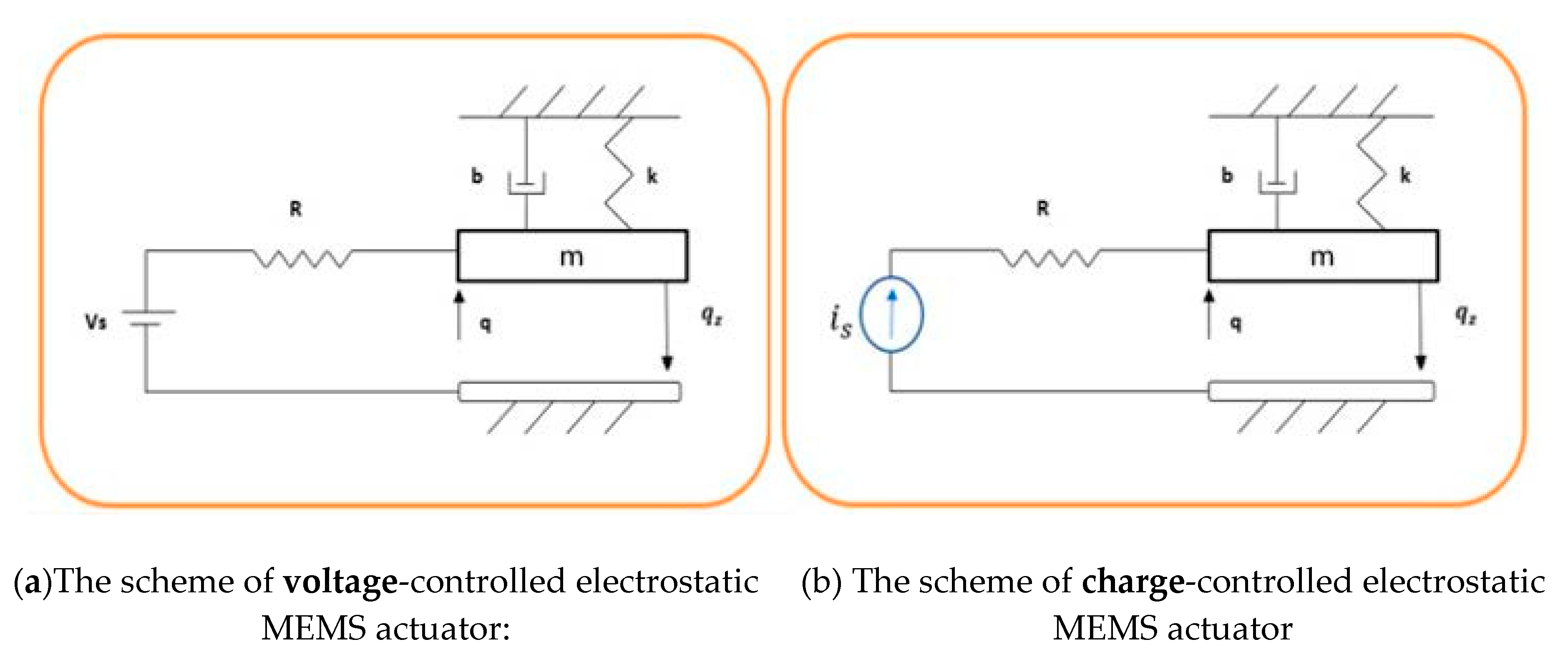
2. The Mathematical Model of the Electrostatic MEMS Actuator

The schematic of an electrostatic actuator is shown in Figure 1 The mechanical subsystem consists of a linear spring with stiffness $k$, a damper with damping coefficient $b$ and a movable plate with mass $m$, while the other plate is fixed. The gap distance is $q\left(t\right)$ and $q_z$ is the distance when the applied voltage is zero. The electrical subsystem consists of a resistor $R$ and a voltage source $V_s$ to drive the system. The mechanical subsystem equation can be found by applying Newton’s second law to the mechanical parts [5,24]:

$$m\ddot{q}\left(t\right)+b\dot{q}\left(t\right)+k\left(q\left(t\right)-q_z\right)=-F_{electric}$$

(1)

where $F_{electric}$ is the electrostatic force which can be given by:

$$F_{electric}=\frac{Q{\left(t\right)}^2}{2Aϵ}$$

(2a)

where $Q\left(t\right)$ is the electric charge, $A$ is the area of the moving plate and $ϵ$ is the electrical permittivity. Using the actuator capacitance $C=Aϵ/q$ and the relationship between the charge and voltage of the parallel plate capacitor $Q=CV$, the electrostatic force can be also represented using voltage representation as

$$F_{electric}=-\frac{AϵV_s^2}{2q^2}$$

(2b)

The electrical subsystem equation can be found by applying Kirchhoff’s voltage law to the circuit [5,24]:

$$\dot{Q}\left(t\right)=\frac{1}{R}\left(V_s-\frac{Q\left(t\right)q\left(t\right)}{Aϵ}\right)$$

(3)

The equations of the system can be found by rearranging (1–3) and defining the states vector as $\left[q,p,Q\right]$^T =$\left[x_1,x_2,x_3\right]$^T where p is the momentum. Thus, the equations can be rewritten as [24]:

$${\dot{x}}_1=\frac{x_2}{m}$$

(4a)

$${\dot{x}}_2=-k\left(x_1-q_z\right)-\frac{b{x}_2}{m}-\frac{x_3^2}{2Aϵ}$$

(4b)

$${\dot{x}}_3=-\frac{x_1{x}_3}{ϵRA}+\frac{V_s}{R}$$

(4c)

In Equation (4c), $V_s$ is the control input $u$. The position of the movable plate is controlled typically via a voltage or charge control depending on the type of the electrical parameter (source) being applied across the parallel plates (capacitor). A voltage-controlled electrostatic MEMS (Figure 1a) uses a voltage source, while for a charged-controlled electrostatic MEMS (Figure 1b) the electrical source is a current source that directly controls the amount of charge on the plates [28].

Here, we adopt the voltage-controlled method. Before proceeding with the analysis and controller design, the equilibrium points of the system must be defined. The equilibria can be estimated by setting (4) to zero, that is

$${\dot{x}}_1=\frac{x_2}{m}=0 \Rightarrow x_2=0$$

(*a)

$${\dot{x}}_2=-k\left(x_1-q_z\right)-\frac{b{x}_2}{m}-\frac{x_3^2}{2Aϵ}=0 \Rightarrow x_3^2=2Akϵ(q_z-x_1)$$

(*b)

$${\dot{x}}_3=\frac{-x_1{x}_3}{ϵRA}+\frac{u}{R}=0 \Rightarrow u=\frac{x_1{x}_3}{Aϵ }$$

(*c)

As discussed in Remark 3.1 and [29], in such a system, which is in fact an underdetermined system, the equilibria are called forced equilibria as the position of the plate can only be maintained by means of a bias voltage or drained current from the input source [30]. Therefore, for any given desired equilibrium (position) $x_{1d} \in \left(0, q_z\right)$ there is a corresponding desired input $u_d$.

For the charge-controlled method, it can also be shown from Equation (*), the equilibrium for a desired position $x_{1d}$, given $x_2=0$, $x_{3d}=\sqrt{2Akϵ(q_z-x_{1d}) }$ and $u_d=V_s{}_d=\frac{x_{1d}{x}_{3d}}{Aϵ }$. When the system is at rest, the voltage $u_d=V_{sd}=0$, which implies the charge ($x_{3d}=0$) and from (*b)  $\Rightarrow x_{1d}=q_z$. For the case of full-gap position when $x_1=0$ and from (*b) $\Rightarrow x_{3d}=\sqrt{2Akϵq_z}$. The equilibrium for the voltage-controlled method is determined based on the pull-in stability phenomenon which will be discussed in Section 3.

Remark 2.1.

Another main difference between the charge and voltage-controlled methods is the type of energy function used to define the generalized effort (electrostatic force) $F_{\mathit{electric}}$ the energy function is used in the case of the charge-controlled method while the co-energy function is used in the voltage-controlled method [31].

To avoid numerical problems, the equations can be normalized as in [5,7,21,24] by defining the states of the system as $\left[X_1,X_2,X_3\right]$ = [$\frac{x1}{\alpha }$, $\frac{\dot{x}1}{\alpha }$, $\frac{x3}{\beta }$], and $\alpha ,\beta$ can be defined as [21]:

$$\alpha =ϵ\sigma AR$$

(5)

$$\beta =ϵ\sigma A\sqrt{\sigma mR}$$

(6)

$$v=\sigma R\beta$$

(7)

where $\sigma$ is the attenuation in the equation $t=\sigma \widehat{t}$. The natural frequency ${\omega }_n$ and the damping ratio $\zeta$ can be defined as:

$${\omega }_n=\sqrt{\frac{k}{m}}$$

(8)

$$2\zeta {\omega }_n=\frac{b}{m}$$

(9)

$$\omega =\frac{{\omega }_n}{\sigma }$$

(10)

Using (5–10) the equations of the normalized system can be rewritten as [21]:

$${\dot{X}}_1=X_2$$

(11a)

$${\dot{X}}_2=-2\zeta \omega X_2-{\omega }^2\left(X_1-q_z\right)-\frac{X_3^2}{2}$$

(11b)

$${\dot{X}}_3=-X_1{X}_3+u.$$

(11c)

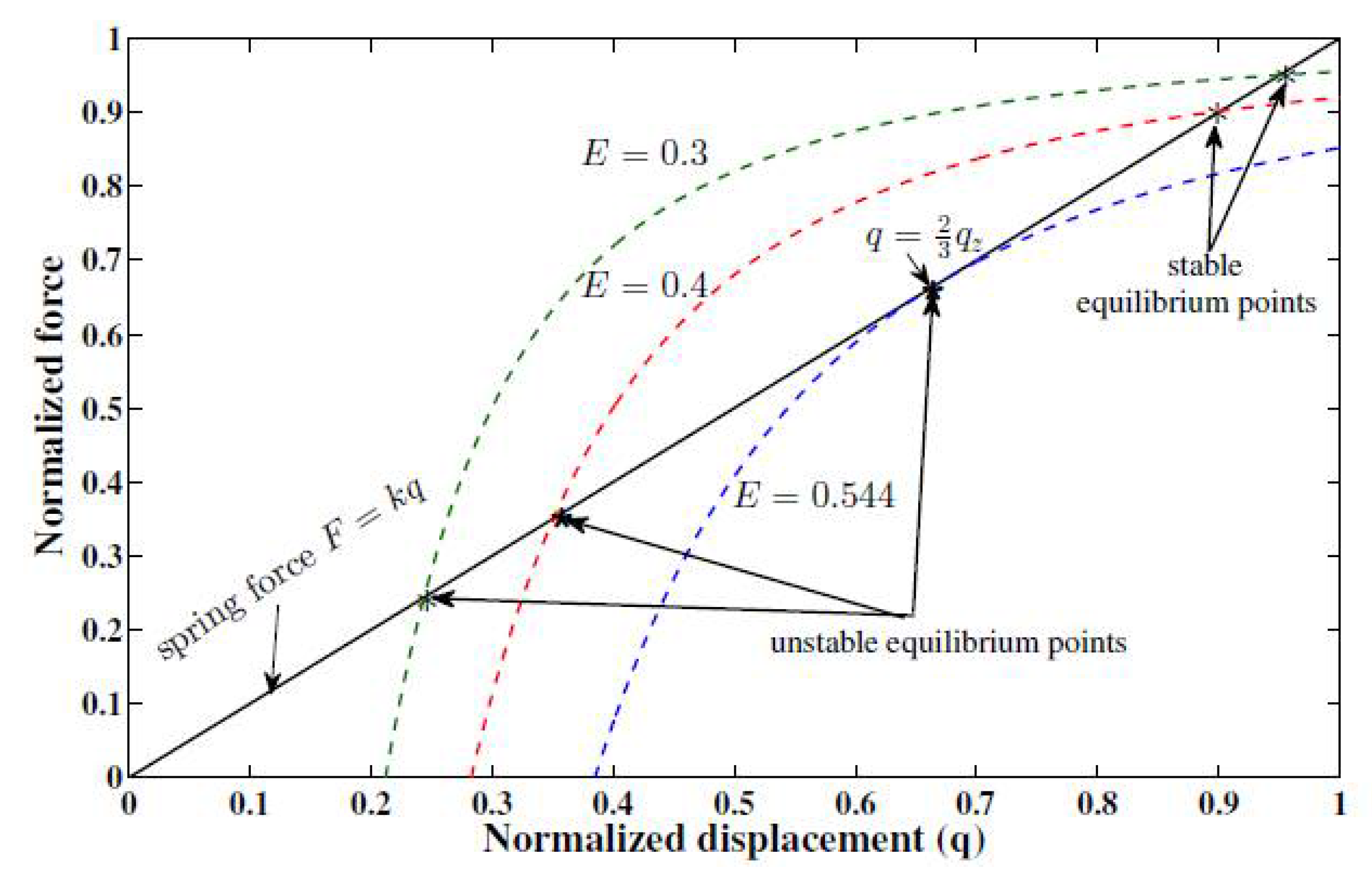
3. The Pull-in Stability Analysis of the System

In this section we investigate the pull-in stability phenomena which is the main challenge in the design and control of the electrostatic MEMS as thoroughly discussed in [1,21,31].

The kinetic energy (KE) of the system is:

$$K\left(x_2\right)=\frac{1}{2m}{x}_2{}^2$$

(12)

and the potential energy (PE) of the system comprises the elastic potential of the linear spring and the electrostatic energy of the capacitor subject to a voltage $V_s$:

$$V\left(x_1\right)=\frac{1}{2}k {\left(x_1-q_z\right)}^2+\frac{AϵV_s^2}{2x_1}=\frac{k}{2}{\left(x_1-q_z\right)}^2+\frac{x_1{x}_3^2}{2Aϵ}$$

(13)

First, we introduce the following remark [25]:

Remark 3.1.

At the desired equilibrium of the EM system, the electrical energy—electrostatic (stored in capacitor) or electromagnetic (stored in inductors)—is never zero as some current has to be drained from the source to keep the mechanical coordinate at some nonzero value [29]. Therefore, the input voltage $V_s$ determines the force, which stretches the spring, thus determines the change in gap. As $V_s$ increases, the charge $x_3$ also increases and the force of attraction between the plates increases, whereas the gap $x_1$ decreases, and thus requires the spring to be stretched from its rest position. Therefore, as shown in Figure 1, at the rest position we have u = $V_s$ = $x_3$ = 0, while the spring is unstretched, in which case $x_1$ = $q_z$. Moreover, the stabilization of this system at any point in the gap is achieved through the balance between the elastic restoring force k($x_1$ − $q_z$) and the electrostatic force $\frac{x_3^2}{2Aϵ}$. Thus, at any forced equilibrium position $x_1$ = $x_{1qq}$ ∈ (0, $q_z$) [31], with $u\left(t\right)=V_{seq}\left(t\right)$ the following must hold:

$$F_{spring}=F_{electric}$$

$$k\left(x_{1eq}-q_z\right)=\frac{x_{3eq}^2}{2Aϵ}=\frac{AϵV_{seq}^2}{2x_{1eq}{}^2}$$

(14)

At some critical voltage when a displacement of the top plate is equal to one-third of the zero-voltage gap, the system becomes unstable and this movable top plate rapidly snaps down to the fixed bottom plate, i.e., the gap collapses to zero. This phenomenon is called “snapthrough” or “pull-in”. Pull-in instability is an inherently nonlinear and crucial undesirable effect. In this section, we perform stability analysis of the MEMS device, and we will show using energy (Hamiltonian) and linearization approaches why the equilibrium of this system is only stable within one-third of the nominal gap. The stability of this actuator is achieved through the balance between the elastic restoring force $k\left(x_1-q_z\right)$ and the electrostatic force (2), which must be equal at equilibrium position $x_{1eq} \in \left(0, q_z\right)$ as in (14). As discussed in [19], a Hamiltonian system is stable if the PE $V \left(q\right)$ has an isolated minimum at the desired equilibrium:

$$x_{1eq}=\arg \min V\left(q\right)$$

(15)

This is satisfied if both ${{\nabla }_{x_1}V|}_{x_1=x_{1eq}}=0$ and ${{\nabla }_{x_1}^{2}V|}_{x_1=x_{1eq}}>0$ hold. The total PE of the system comprises the elastic potential of the linear spring and the electrostatic energy

$$V\left(x_1\right)=\frac{1}{2}k {\left(x_1-q_z\right)}^2+\frac{AϵV_{seq}^2}{2x_1}$$

(16)

Substituting $V_{seq}^2$ from (14) into (13), we obtain:

$$V\left(x_1\right)=\frac{1}{2}k {\left(x_1-q_z\right)}^2+\frac{k{x}_{1eq}^2\left(x_{1eq}-q_z\right)}{x_1}$$

(17)

Therefore,

$${{\nabla }_{x_1}^{2}V|}_{x_1=x_{1eq}}=k\left(1+\frac{2\left(x_{1eq}-q_z\right)}{x_{1eq}}\right)=k\left(3-\frac{2q_z}{x_{1eq}}\right)>0 \to x_{1eq}>\frac{2}{3}{q}_z$$

(18)

From (18), the Hessian is only positive if $x_{1eq}>\frac{2}{3}{q}_z$. Thus, the energy function has a local minimum at $x_{1eq}>\frac{2}{3}{q}_z$, which is the upper one-third region of the gap.

The stability analysis of the MEMS device can also be shown using linearization. The equilibria are determined by finding the solution so that the original state equations are zero, i.e., solving the following set of equations:

$${\dot{x}}_1=\frac{x_2}{m}=0$$

(19a)

$${\dot{x}}_2=-k\left(x_1-q_z\right)-\frac{b{x}_2}{m}-\frac{x_3^2}{2Aϵ}=0$$

(19b)

$${\dot{x}}_3=\frac{-x_1{x}_3}{ϵRA}+\frac{u}{R}=0$$

(19c)

Thus, we obtain:

$$x_2=0$$

(20a)

$$x_1=q_z-\frac{x_3^2}{2Akϵ}$$

(20b)

$$x_3=\frac{u}{Aϵx_1 }$$

(20c)

Substituting (20c) into (20b) yields:

$$x_1^3-q_z{x}_1^2+\frac{u^2}{c_0}=0; c_0=2k{\left(Aϵ\right)}^3$$

(21)

There are three solutions for (21); one is negative for positive input voltages and can thus be ignored. The other two solutions are both positive. One of these equilibria is stable and the other is unstable. The stability of the system can also be analyzed by applying Lyapunov’s indirect method [32] to the system (4), which gives:

$$A=\left[\begin{array}{ccc}0& \frac{1}{m}& 0\\ -k& -\frac{b}{m}& -\frac{x_3}{Aϵ}\\ -\frac{x_3}{RAϵ}& 0& -\frac{x_1}{RAϵ}\end{array}\right]$$

(22)

The eigenvalues of $A$ are the solutions ${\lambda }_i$ of

$$\left|\begin{array}{ccc}\lambda & -\frac{1}{m}& 0\\ k& \lambda +\frac{b}{m}& \frac{x_3}{Aϵ}\\ \frac{x_3}{RAϵ}& 0& \lambda +\frac{x_1}{RAϵ}\end{array}\right|={\lambda }^3+\left(\frac{x_1}{RAϵ}+\frac{b}{m}\right){\lambda }^2+\left(\frac{b{x}_1}{RAϵm}+\frac{k}{m}\right)\lambda +\frac{k{x}_1}{RAϵm}-\frac{x_3^2}{R{\left(Aϵ\right)}^{2}m}=0$$

(23)

Substitute $-x_3^2=2kAϵ\left(x_1-q_z\right)$ from (20b) into (23) gives:

$${\lambda }^3+\left(\frac{x_1}{RAϵ}+\frac{b}{m}\right){\lambda }^2+\left(\frac{b{x}_1}{RAϵm}+\frac{k}{m}\right)\lambda +\frac{k}{RAϵm}\left(3x_1-2q_z\right)=0$$

(24)

As all parameters, thus coefficients, are positive, the condition for negative eigenvalues is that $3x_1-2q_z>0,$ hence:

$$x_{1eq}>\frac{2}{3}{q}_z$$

i.e., the system is only stable within one third of its full gap and the region of stability is $x_1 \in \left(\frac{2}{3}{q}_z,q_z\right)$.

The explanation of the “pull-in” phenomenon is that the stability of the system at equilibrium is governed by two forces; the electrostatic force applied to the movable plate that pulls the plate down and the elastic stiffness (spring force) that pulls the spring, thus the top plate, up. Therefore, (14) is satisfied at the equilibrium. From (14) with the spring force constant $k=1$ and using (21), we can plot, as in Figure 2, the relationship between the spring force (straight line) and the electrostatic force (curved line), for various values of the input voltage u.

As shown, there are two intersections, which means two equilibria; one is stable, and one is unstable (saddle-node) [5]. When the upper plate’s deflection $q \left(x_1\right)$ is less than one-third of the zero voltage gap $q_z$, and with small perturbation of the gap, the actuator returns to its equilibrium point as the increase in the restoring force of the linear spring is greater than the increase in the electrostatic force. As $q\ge \frac{1}{3}{q}_z$, any perturbation will result in the attractive electrostatic force being the dominant force, hence causing the top plate to collapse to the fixed plate. For voltage values above the pull-in limit, there is no equilibrium point (the curves never intersect).

Due to the pull-in instability which is inherited behavior of voltage-controlled actuators, the equilibrium can be obtained once the desired stable position point ($x_{1d}=x_{1eq})$ is identified. For a given position $x_{1d}$ along with its corresponding given constant voltage ($V_s{}_d$), the charge is obtained as:

$$x_{3eq}=C{V}_s{}_d=\frac{Aϵ}{x_{1eq}}{V}_s{}_d$$

In this paper, we are interested in the stabilization of the system over the entire gap position, i.e., the forced equilibrium

$$\left(x_{1eq},x_{2eq,}{x}_{3eq}\right)=\left(x_{1d},0,\frac{Aϵ}{x_{1d}}{V}_s{}_d\right).$$

4. Design of the Controller and the Observer for the MEMS Actuator

4.1. The Port-Hamiltonian Model of the System

The port-Hamiltonian of dynamic systems can be defined as [19]:

$$\dot{x}=\left[J\left(x\right)-R\left(x\right)\right]\nabla H+g\left(x\right)u,$$

$$y=g{\left(x\right)}^T\nabla H$$

(25)

where x $\in R^n$ is the states vector, H is the Hamiltonian function H:$R^n\to R$, $\nabla H$ is the gradient vector of $H$, $u$ is the control input of the system, $J\left(X\right)$ is the interconnection matrix with $J\left(x\right)=-J{\left(x\right)}^T$, R(x) is the damping matrix with $R\left(x\right)=R{\left(x\right)}^T\ge 0$ and $g\left(x\right)$ is the input matrix. The port-Hamiltonian model of the MEMS system (4) can be defined as [24]:

$$\left[\begin{array}{c}{\dot{x}}_1\\ {\dot{x}}_2\\ {\dot{x}}_3\end{array}\right]=\left[\begin{array}{ccc}0& 1& 0\\ -1& -b& 0\\ 0& 0& -\frac{1}{R}\end{array}\right]\left[\begin{array}{c}{\nabla }_{x_1}H\\ {\nabla }_{x_2}H\\ {\nabla }_{x_3}H\end{array}\right]+\left[\begin{array}{c}0\\ 0\\ \frac{1}{R}\end{array}\right]u$$

(26)

$$y=g{\left(x\right)}^T\nabla H.$$

Moreover, the Hamiltonian (energy function) of the system is defined as:

$$H=\frac{1}{2}k{\left(x_1-q_z\right)}^2+\frac{x_2^2}{2m}+\frac{x_1{x}_3^2}{2Aϵ}$$

(27)

4.2. The Controller Design Based on IDA-PBC Method

The main target of IDA-PBC is to find the control law $u$ by matching the open-loop system (26) with the desired closed loop system which can be given by:

$$\dot{x}=\left[J_d\left(x\right)-R_d\left(x\right)\right]\nabla H_d$$

$$y_d=g{\left(x\right)}^T\nabla H_d$$

(28)

The following can be designed to stabilize the system and to meet the required performance of the system: $J_d\left(x\right),R_d\left(x\right)$ and $H_d$ are the desired interconnection matrix, the desired damping matrix and the desired Hamiltonian, respectively. Here, we show the design of the controller based on [25], but we add coupling between the momentum state and the charge state via the interconnection matrix and state transformations as concluded in the following proposition:

Proposition 5.1.

The electrostatic MEMS actuator model (26) can be controlled and stabilized at the equilibrium point ($x_{1eq}$, 0,$x_{3eq}$by the following dynamic control law u:

$$\begin{array}{c}u=\frac{R\Gamma }{x_3}\frac{-\left(\frac{\gamma x_1}{Aϵ}+\gamma K_1\right)-\sqrt{{\left(\frac{\gamma x_1}{Aϵ}+\gamma K_1\right)}^2+\frac{2}{Aϵ}\left(z_4+\frac{x_3^2}{2Aϵ}\right)}}{\frac{-1}{Aϵ}}+\frac{R{\gamma }^2{x}_1{x}_2}{m{x}_3}+\frac{R{x}_2{\gamma }^2{K}_{1}Aϵ}{m{x}_3}\\ +\frac{RAϵK_i{x}_2}{m{x}_3}+\frac{x_3{x}_1}{Aϵ}\end{array}$$

(29)

$${\dot{z}}_4=-K_i{\nabla }_{z_2}{H}_d,$$

with

$$\begin{array}{c}\Gamma =(-\gamma \frac{2x_2}{m}-K_v\frac{-\left(\frac{\gamma x_1}{Aϵ}+\gamma K_1\right)-\sqrt{{\left(\frac{\gamma x_1}{Aϵ}+\gamma K_1\right)}^2+\frac{2}{Aϵ}\left(z_4+\frac{x_3^2}{2Aϵ}\right)}}{\frac{-1}{Aϵ}}\left(\frac{x_1}{Aϵ}+K_1\right)\\ +\gamma x_1{K}_v\left(\frac{x_1}{Aϵ}+K_1\right)+\gamma K_{1}AϵK_v\left(\frac{x_1}{Aϵ}+K_1\right),\end{array}$$

and the desired Hamiltonian of the system:

$$H_d=\frac{1}{2}k{\left(z_1-q_z\right)}^2+\frac{z_2^2}{2m}+\frac{z_1{z}_3^2}{2Aϵ}+\frac{1}{2}{K}_1{z}_3^2+\frac{1}{2}{K}_i{}^{-1}{z}_4^2$$

(30)

where $K_i>0$ is the integral term, and $K_1>0$ is a constant to stabilize the system. The port-Hamiltonian system of the closed loop system is given by:

$$\left[\begin{array}{c}{\dot{z}}_1\\ {\dot{z}}_2\\ \begin{array}{c}{\dot{z}}_3\\ {\dot{z}}_4\end{array}\end{array}\right]=\left[\begin{array}{cc}\begin{array}{cc} 0& 1\\ -1& -b\end{array}& \begin{array}{cc} 0& 0\\ \gamma & K_i\end{array}\\ \begin{array}{cc} 0 & -\gamma \\ 0& -K_i\end{array}& \begin{array}{cc}-K_v& 0\\ 0& 0\end{array}\end{array}\right]\left[\begin{array}{c}{\nabla }_{z_1}{H}_d\\ {\nabla }_{z_2}{H}_d\\ \begin{array}{c}{\nabla }_{z_3}{H}_d\\ {\nabla }_{z_4}{H}_d\end{array}\end{array}\right]$$

(31)

where $\gamma$ is a constant coupling term between the momentum and the electric charge, being the essential difference between the interconnection matrix in this design and the interconnection matrix in [25]. The term $K_v>0$ is the damping term to asymptotically stabilize the system. The coordinate transformations are defined by:

$$z_1=x_1; z_{2 }=x_2;$$

$$z_3=\frac{-\left(\frac{\gamma z_1}{Aϵ}+\gamma K_1\right)-\sqrt{{\left(\frac{\gamma z_1}{Aϵ}+\gamma K_1\right)}^2+\frac{2}{Aϵ}\left(z_4+\frac{x_3^2}{2Aϵ}\right)}}{\frac{-1}{Aϵ}}$$

(32)

Proof of Proposition 5.1.

The desired Hamiltonian function (30) can be chosen as a Lyapunov candidate. The time derivative of this function along the trajectories of (31) is given by:

$$\begin{array}{c}{\dot{H}}_d={\nabla }_{z_1}{H}_d{\dot{z}}_1+{\nabla }_{z_2}{H}_d{\dot{z}}_2+{\nabla }_{z_3}{H}_d{\dot{z}}_3+{\nabla }_{z_4}{H}_d{\dot{z}}_4\\ ={\nabla }_{z_1}{H}_d{\nabla }_{z_2}{H}_d+{\nabla }_{z_2}{H}_d\left(-{\nabla }_{z_1}{H}_d-b{\nabla }_{z_2}{H}_d+\gamma {\nabla }_{z_3}{H}_d+K_i{\nabla }_{z_4}{H}_d\right)\\ +{\nabla }_{z_3}{H}_d\left(-\gamma {\nabla }_{z_2}{H}_d-K_v{\nabla }_{z_3}{H}_d\right)+{\nabla }_{z_4}{H}_d\left(-K_i{\nabla }_{z_2}{H}_d\right)\\ =-b{\left|{\nabla }_{z_2}{H}_d\right|}^2-K_v{\left|{\nabla }_{z_3}{H}_d\right|}^2\\ =-b{\left|\frac{z_2}{m}\right|}^2-K_v{\left|\frac{z_1{z}_3}{Aϵ}+K_1{z}_3\right|}^2 \le 0\end{array}$$

(33)

which is negative semi-definite, i.e., the system is stable. Furthermore, asymptotic stability at the desired equilibrium can be verified by imposing the following detectability condition [33]:

Condition 1:

The output $y_d=\left[\begin{array}{c}\frac{z_2}{m}\\ \frac{z_1{z}_3}{Aϵ}+K_1{z}_3\end{array}\right]$ of the closed-loop system (31) is detectable. □

Applying the detectability Condition 1 and given (33), asymptotic stability is guaranteed. The controller (29) is found using the transformation (32); that is, taking the derivate of the second transformation:

$${\dot{x}}_2={\dot{z}}_2$$

$$-{\nabla }_{x_1}H-b{\nabla }_{x_2}H=-{\nabla }_{z_1}{H}_d-b{\nabla }_{z_2}{H}_d+\gamma {\nabla }_{z_3}{H}_d+K_i{\nabla }_{z_4}{H}_d$$

$$-k\left(x_1-q_z\right)-\frac{x_3^2}{2Aϵ}-\frac{b{x}_2}{m}=-k\left(z_1-q_z\right)-\frac{z_3^2}{2Aϵ}-\frac{b{z}_2}{m}+\gamma \left(\frac{z_1{z}_3}{Aϵ}+K_1{z}_3\right)+z_4$$

$$z_3^2\left(\frac{-1}{2Aϵ}\right)+z_3\left(\frac{z_1\gamma }{Aϵ}+K_1\gamma \right)+\left(z_4+\frac{x_3^2}{2Aϵ}\right)=0$$

(34)

This equation is quadratic in $z_3$ and the solution can be found by the general law of quadratic equations. By rearranging the third transformation and taking its derivate with respect to time we get:

$$z_3=\frac{-\left(\frac{\gamma z_1}{Aϵ}+\gamma K_1\right)-\sqrt{{\left(\frac{\gamma z_1}{Aϵ}+\gamma K_1\right)}^2+\frac{2}{Aϵ}\left(z_4+\frac{x_3^2}{2Aϵ}\right)}}{\frac{-1}{Aϵ}}$$

$$\frac{z_3}{Aϵ}=\frac{\gamma z_1}{Aϵ}+\gamma K_1+\sqrt{{\left(\frac{\gamma z_1}{Aϵ}+\gamma K_1\right)}^2+\frac{2}{Aϵ}\left(z_4+\frac{x_3^2}{2Aϵ}\right)}$$

$${\left(\frac{z_3}{Aϵ}-\frac{\gamma z_1}{Aϵ}-\gamma K_1\right)}^2={\left(\frac{\gamma z_1}{Aϵ}+\gamma K_1\right)}^2+\frac{2}{Aϵ}\left(z_4+\frac{x_3^2}{2Aϵ}\right)$$

$$2\left(\frac{z_3}{Aϵ}-\frac{\gamma z_1}{Aϵ}-\gamma K_1\right)\left(\frac{{\dot{z}}_3}{Aϵ}-\frac{\gamma {\dot{z}}_1}{Aϵ}\right)=2\left(\frac{\gamma z_1}{Aϵ}+\gamma K_1\right)\frac{\gamma {\dot{z}}_1}{Aϵ}+\frac{2{\dot{z}}_4}{Aϵ}+\frac{2x_3{\dot{x}}_3}{A^2{ϵ}^2}$$

$$\frac{z_3{\dot{z}}_3}{A^2{ϵ}^2}-\frac{\gamma {\dot{z}}_1{z}_3}{A^2{ϵ}^2}-\frac{{\dot{z}}_3\gamma z_1}{A^2{ϵ}^2}+\frac{{\gamma }^2{z}_1{\dot{z}}_1}{A^2{ϵ}^2}-\frac{{\dot{z}}_3\gamma K_1}{Aϵ}+\frac{{\dot{z}}_1{\gamma }^2{K}_1}{Aϵ}=\frac{{\gamma }^2{z}_1{\dot{z}}_1}{A^2{ϵ}^2}+\frac{{\dot{z}}_1{\gamma }^2{K}_1}{Aϵ}+\frac{{\dot{z}}_4}{Aϵ}+\frac{x_3{\dot{x}}_3}{A^2{ϵ}^2}$$

$$\gamma {\dot{z}}_1{z}_3+{\dot{z}}_3{z}_3-\gamma {\dot{z}}_3{z}_1-{\dot{z}}_3\gamma K_{1}Aϵ={\dot{z}}_{4}Aϵ+x_3{\dot{x}}_3$$

(35)

$$-\gamma {\dot{z}}_1{z}_3+{\dot{z}}_3{z}_3-\gamma {\dot{z}}_3{z}_1-{\dot{z}}_3\gamma K_{1}Aϵ={\dot{z}}_{4}Aϵ+x_3\frac{1}{R}\left(u-\frac{x_3{x}_1}{Aϵ}\right)$$

$$\begin{array}{c}-\gamma \frac{z_2}{m}{z}_3-\frac{\gamma z_2{z}_3}{m}-z_3{K}_v\left(\frac{z_1{z}_3}{Aϵ}+z_3{K}_1\right)+\frac{{\gamma }^2{z}_1{z}_2}{m}+\gamma z_1{K}_v\left(\frac{z_1{z}_3}{Aϵ}+z_3{K}_1\right)+\frac{z_2{\gamma }^2{K}_{1}Aϵ}{m}\\ +\gamma K_{1}AϵK_v\left(\frac{z_1{z}_3}{Aϵ}+z_3{K}_1\right)=-K_i\frac{z_2}{m}Aϵ+x_3\frac{1}{R}\left(u-\frac{x_3{x}_1}{Aϵ}\right)\end{array}$$

$$\begin{array}{c}{z}_3\left(-\gamma \frac{2x_2}{m}-K_v\left(\frac{x_1{z}_3}{Aϵ}+z_3{K}_1\right)+\gamma x_1{K}_v\left(\frac{x_1}{Aϵ}+K_1\right)+\gamma K_{1}AϵK_v\left(\frac{x_1}{Aϵ}+K_1\right)\right)+\frac{{\gamma }^2{x}_1{x}_2}{m}\\ +\frac{x_2{\gamma }^2{K}_{1}Aϵ}{m}=-K_i\frac{x_2}{m}Aϵ+x_3\frac{1}{R}\left(u-\frac{x_3{x}_1}{Aϵ}\right)\end{array}$$

By rearranging and compensating the transformations, we obtain the control law (29).

Remark 5.1.

By comparing the proposed method with that in [25], we notice that in this method we obtain a simpler control law and the transformation has been applied onto one coordinate (state): only on (x₃). In [25], the transformation has been applied onto all states (x₁, x₂, x₃).

Remark 5.2.

By inspecting the controller (29), we notice the presence of the momentum (speed) state (due to a coupling which is another improvement) which is practically difficult to measure using special sensors [10]. In the following, we show the construction of the speed observer.

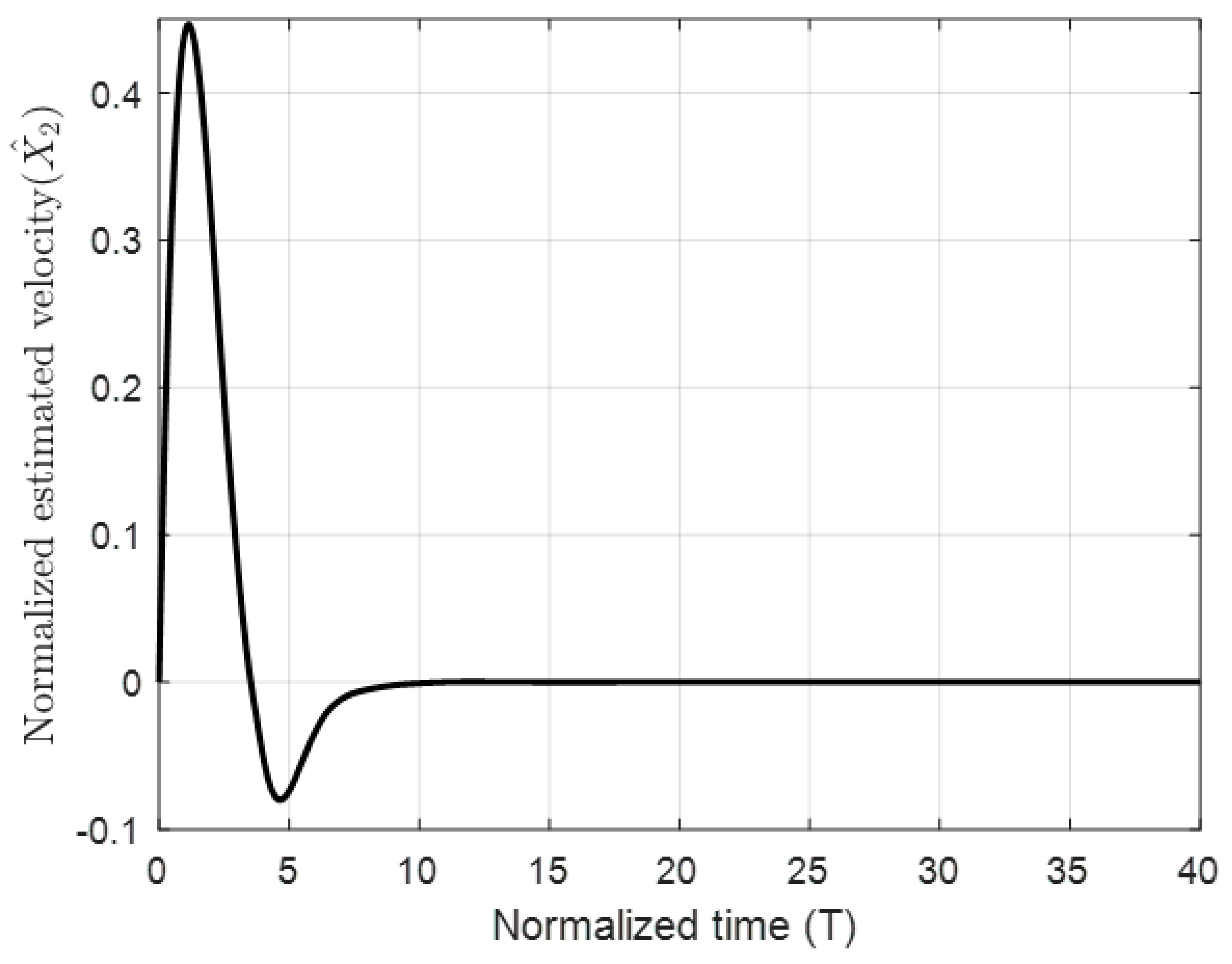
4.3. The Design of the Speed Observer

Finally, the speed ($v$) in the MEMS actuator is difficult to measure, so a speed observer can be used to estimate the speed and then the momentum (the state in the port-controlled Hamiltonian formalism) is found using

$$p=x_2=mv.$$

The form of the speed observer ($O$) is taken from [10] which is:

$$O=x_2-k_2{x}_1,$$

(36)

where $k_2$ is a constant. We take the derivative of both sides of (36) with respect to time:

$$\dot{O}={\dot{x}}_2-k_2{\dot{x}}_1$$

(37)

Substituting the terms from (4) into (37), yields:

$$\dot{O}=-k\left(x_1-q_z\right)-\frac{b\left(O+k_2{x}_1\right)}{m}-\frac{x_3^2}{2Aϵ}-k_2{\dot{x}}_1$$

(38)

The estimate of the $O$ is formulated as

$$\dot{\widehat{O}}=-k\left(x_1-q_z\right)-\frac{b\left(\widehat{O}+k_2{x}_1\right)}{m}-\frac{x_3^2}{2Aϵ}-k_2{\dot{x}}_1$$

(39)

Finally, the estimate of the speed $x_2$ is given by:

$${\widehat{x}}_2=\widehat{O}+k_2{x}_1$$

(40)

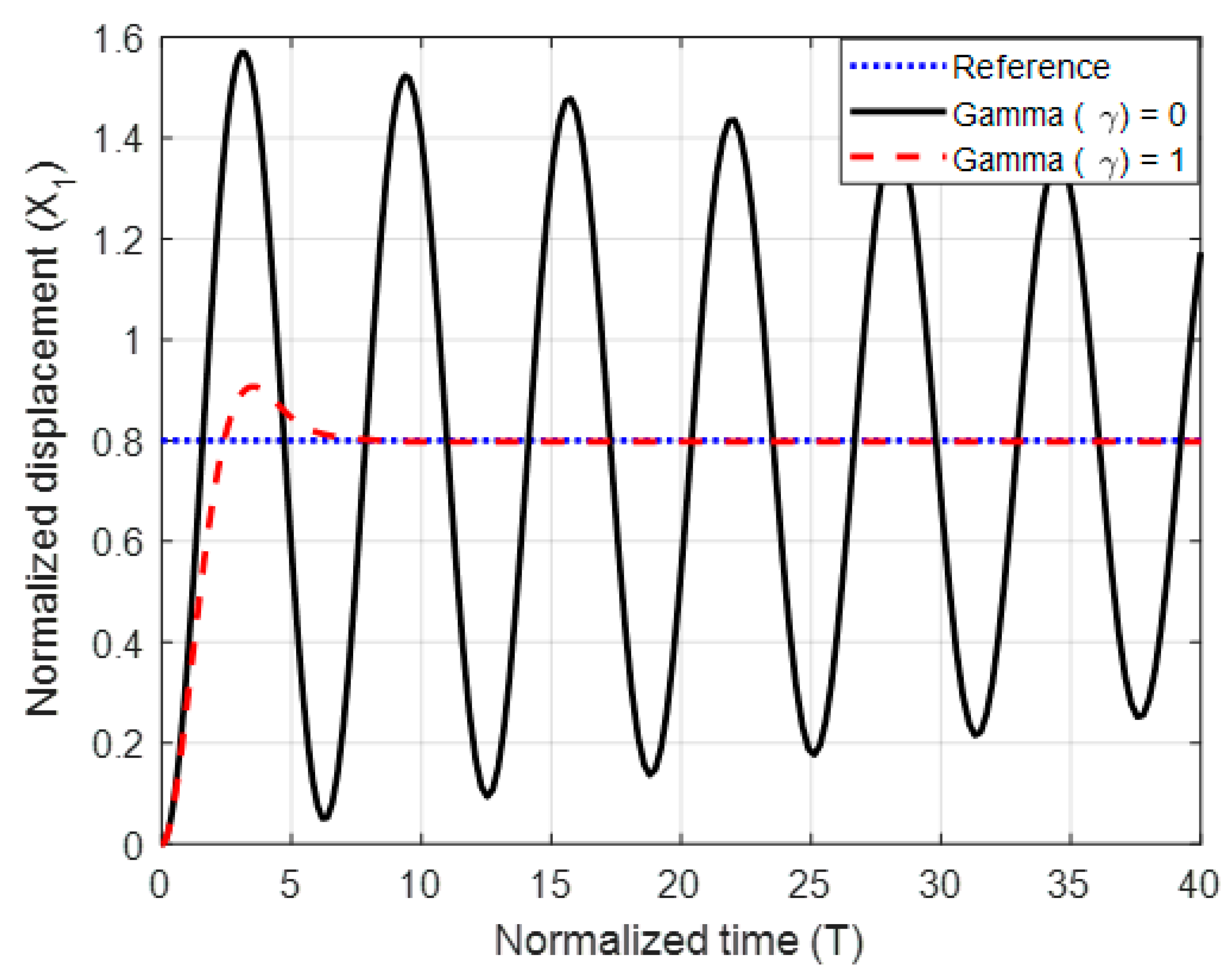
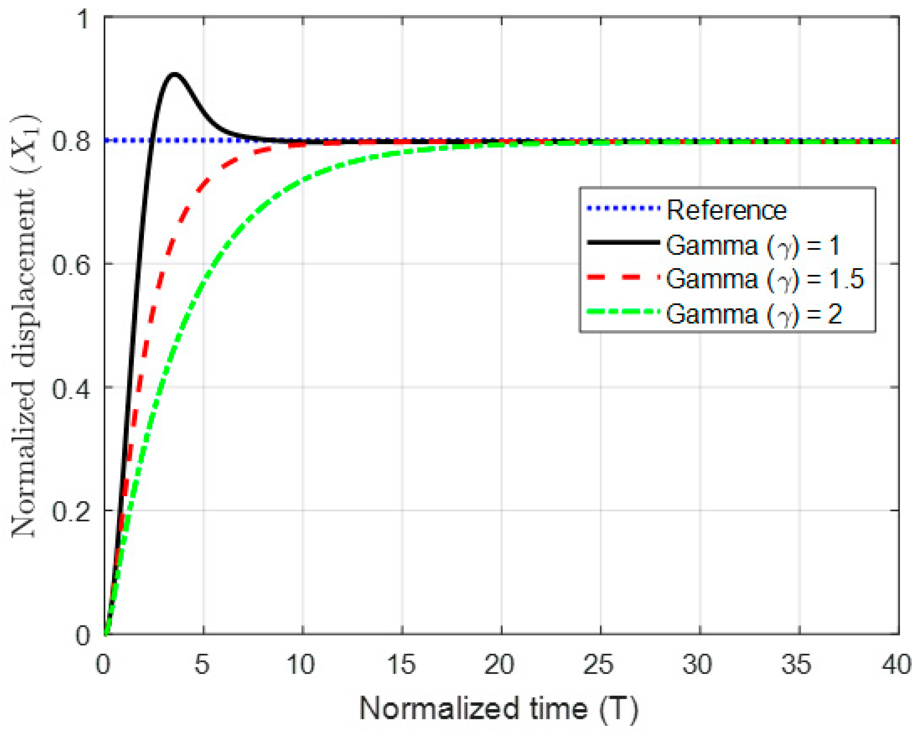
5. Numerical Simulations

The obtained theoretical results were validated through two numerical simulation environments: the MATLAB/Simulink environment was used to simulate the parallel plate MEMS actuator, and Multiphysics modelling software COMSOL (5.5) was used to simulate the radio frequency (RF) MEMS device.

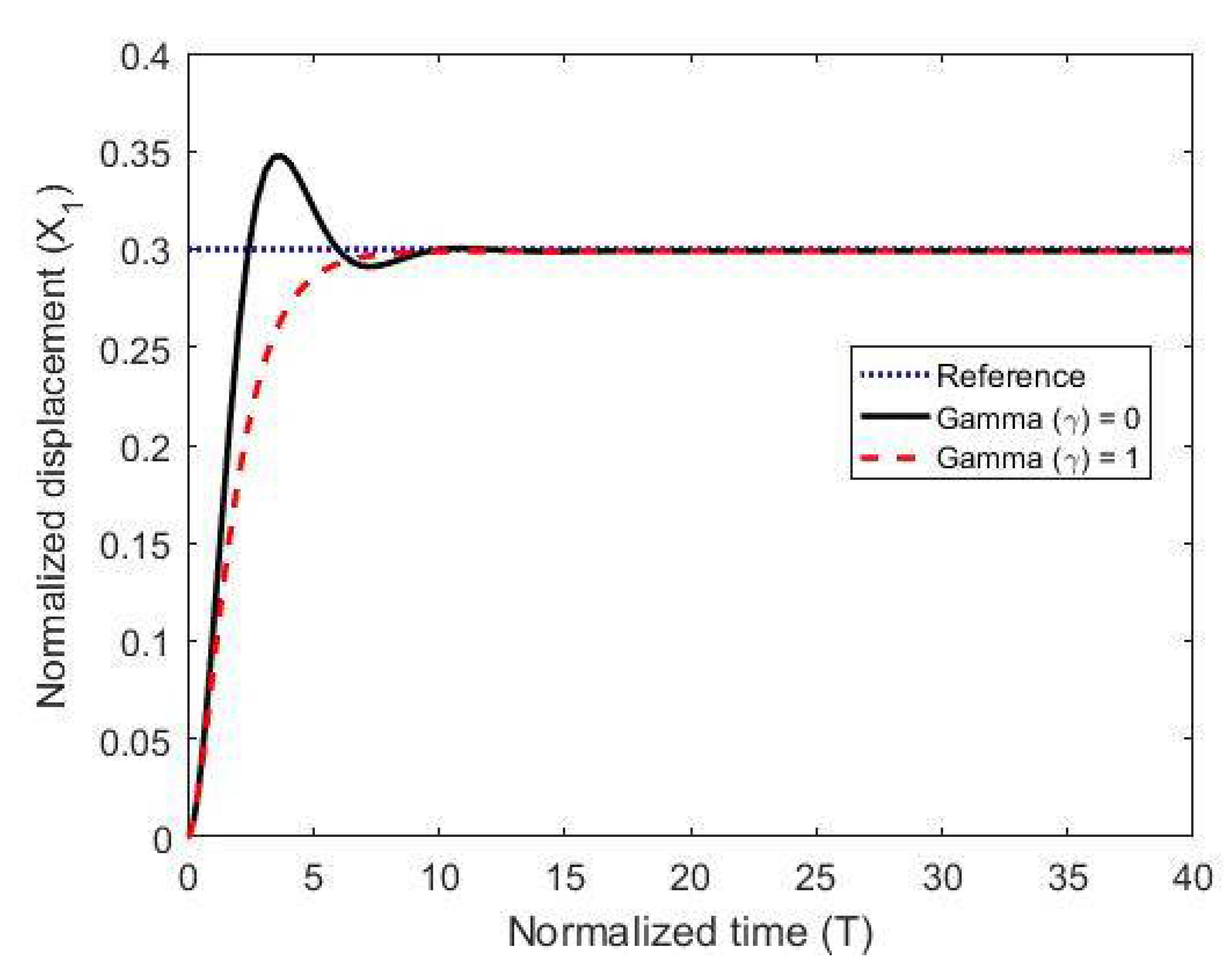
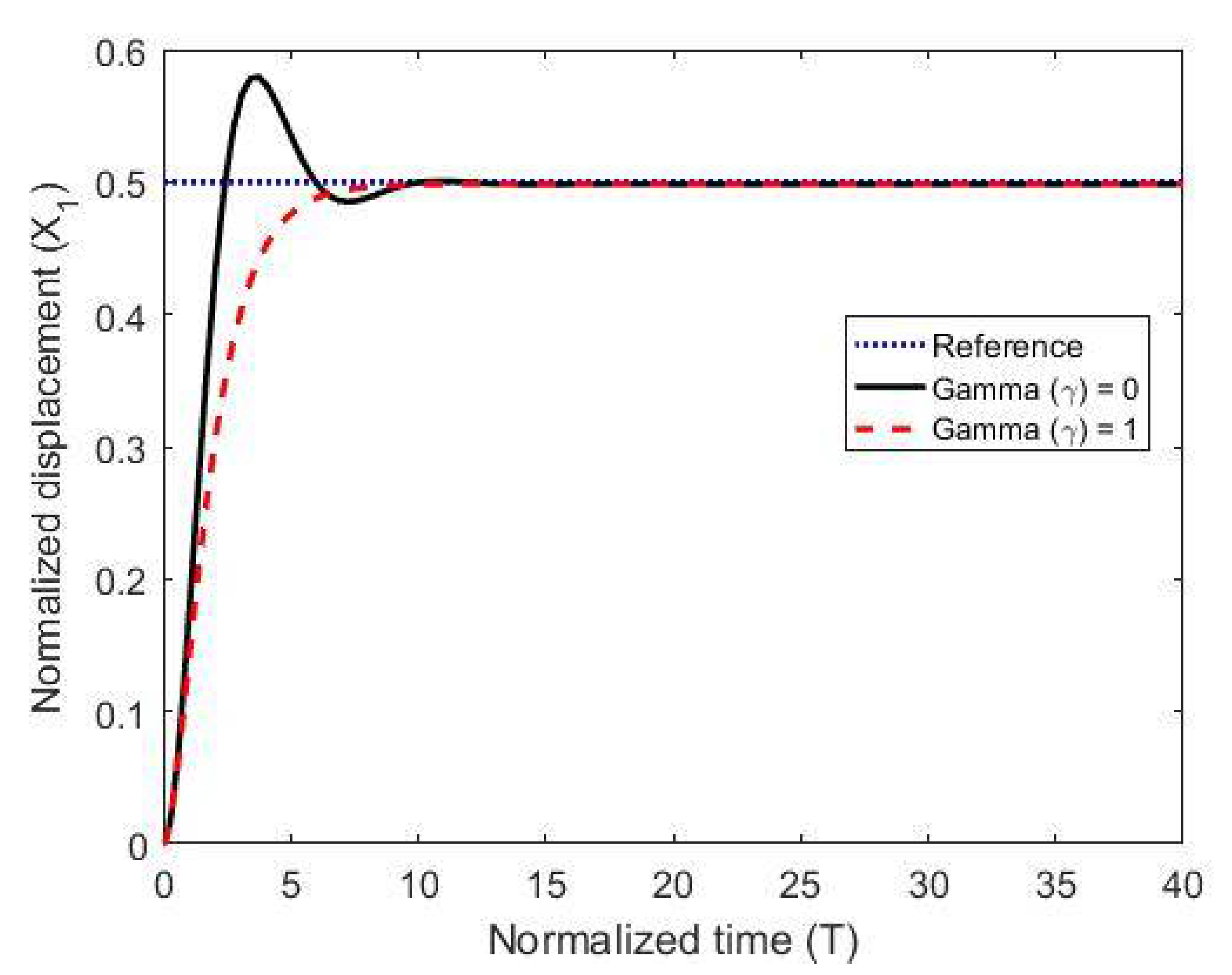
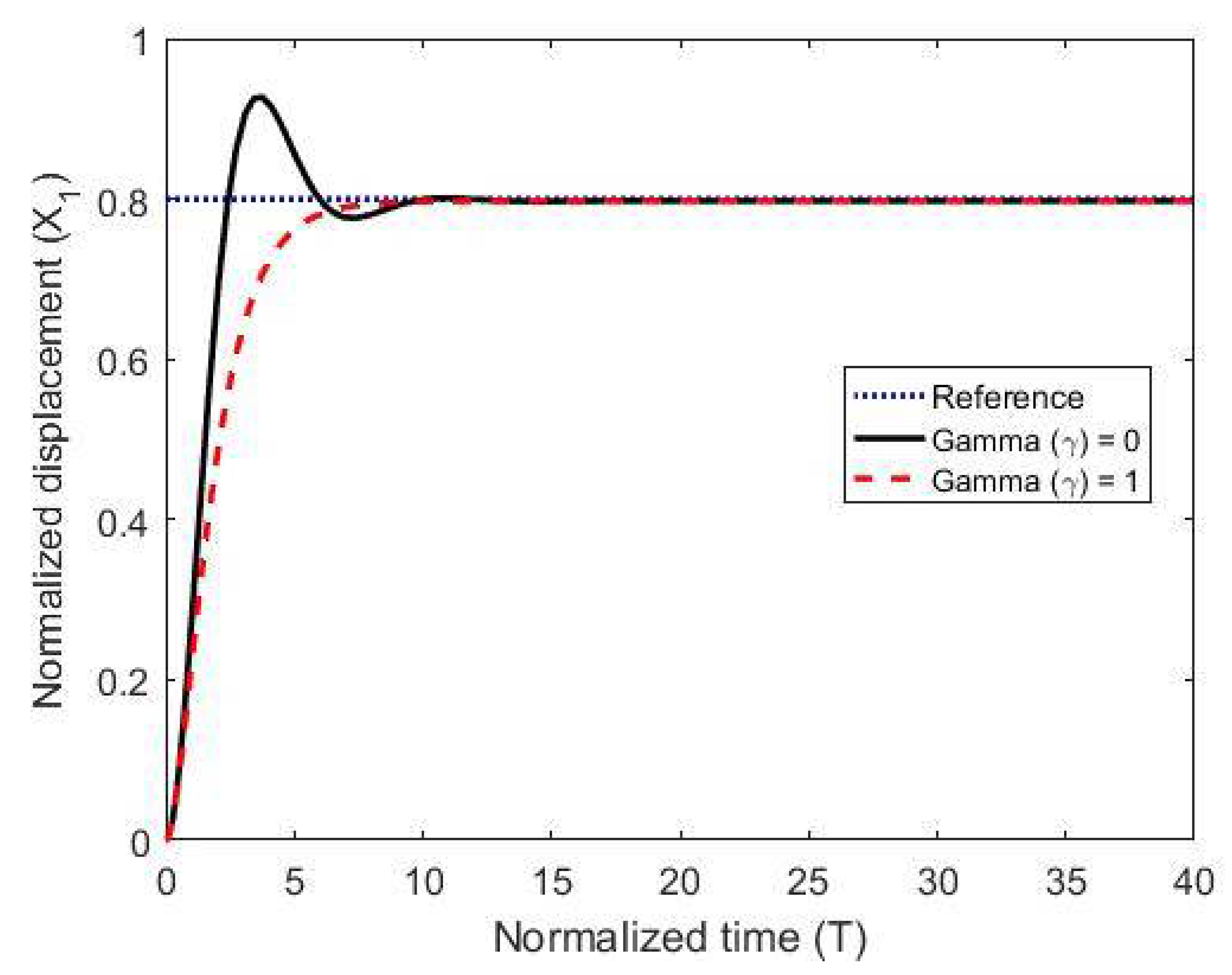
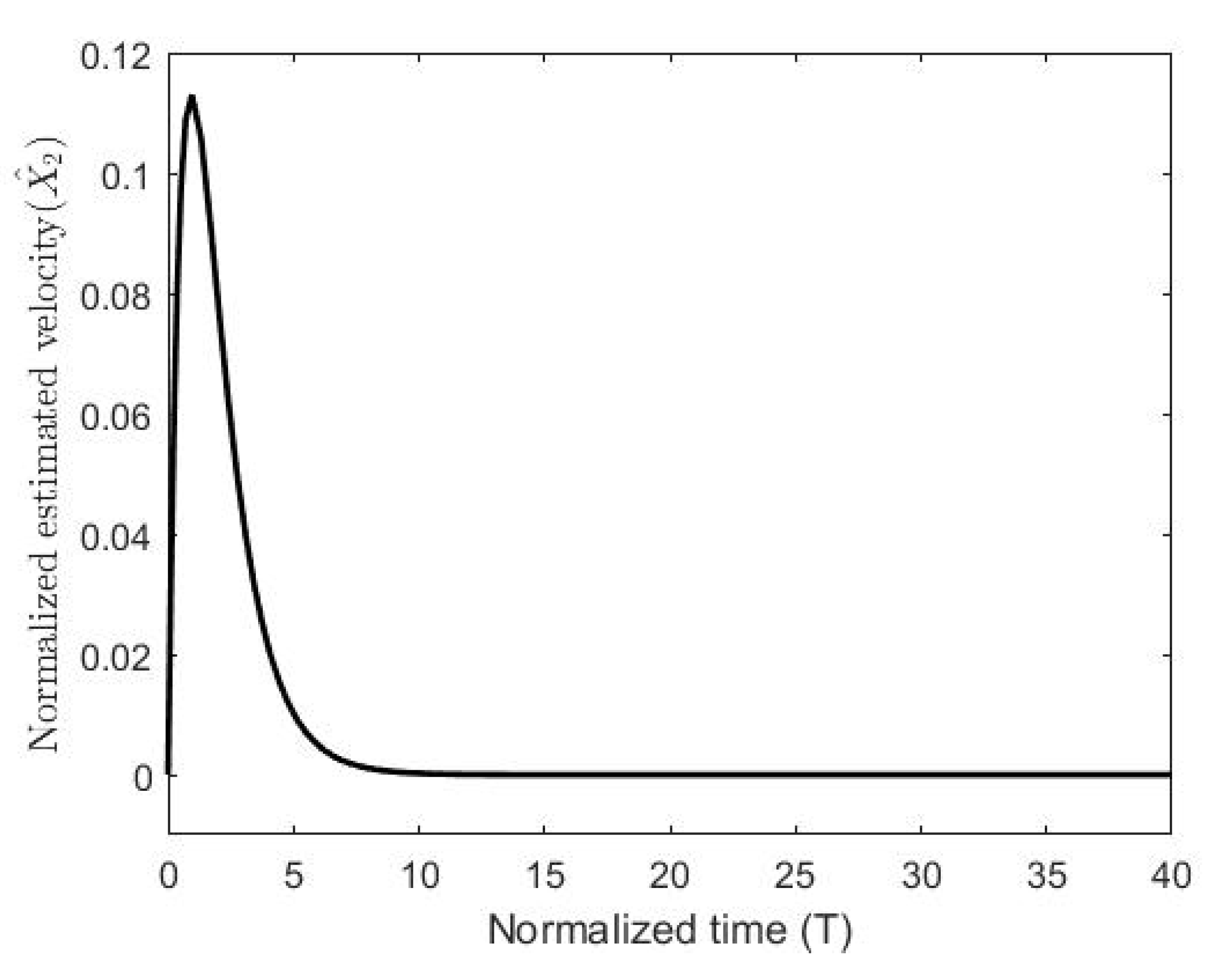
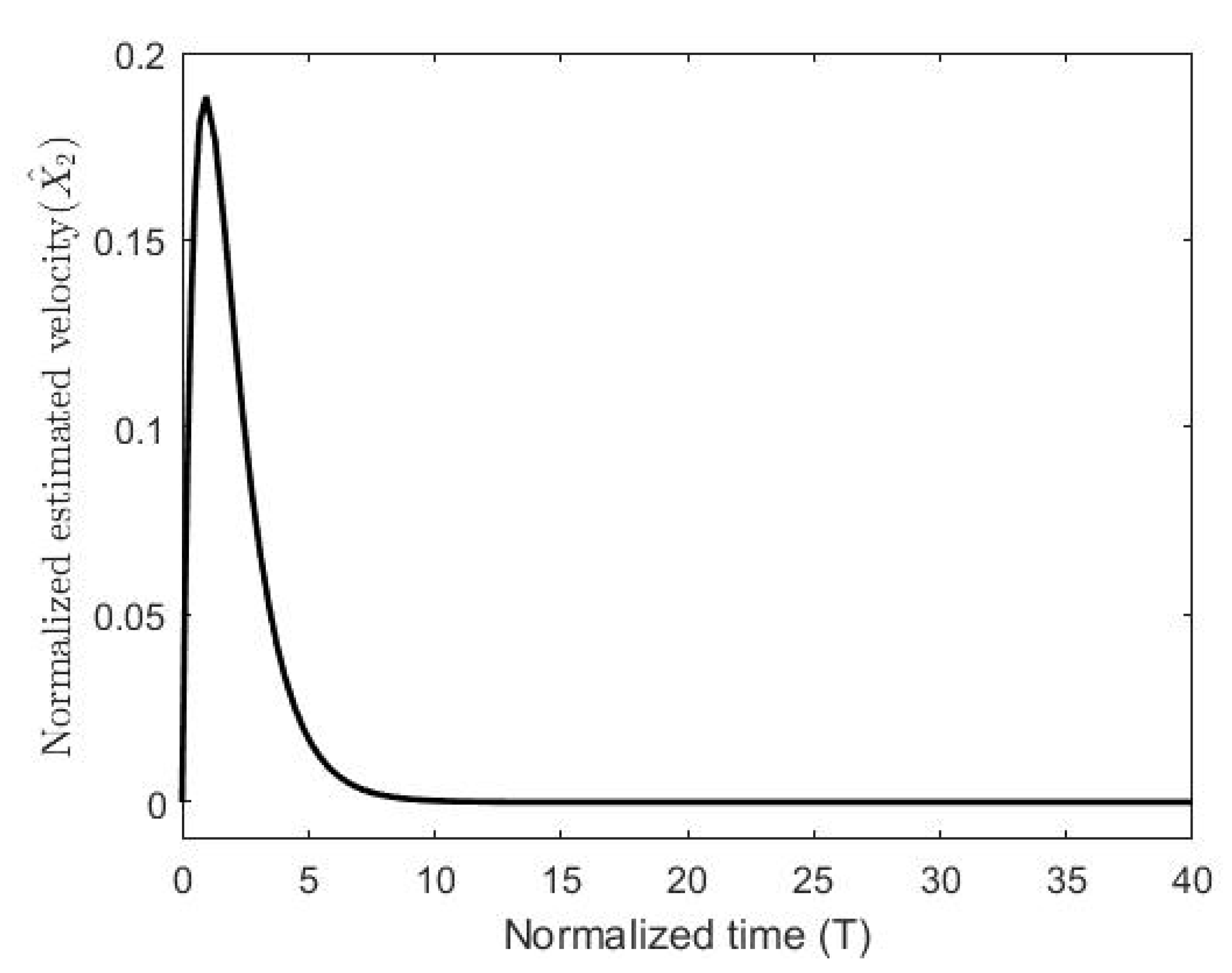
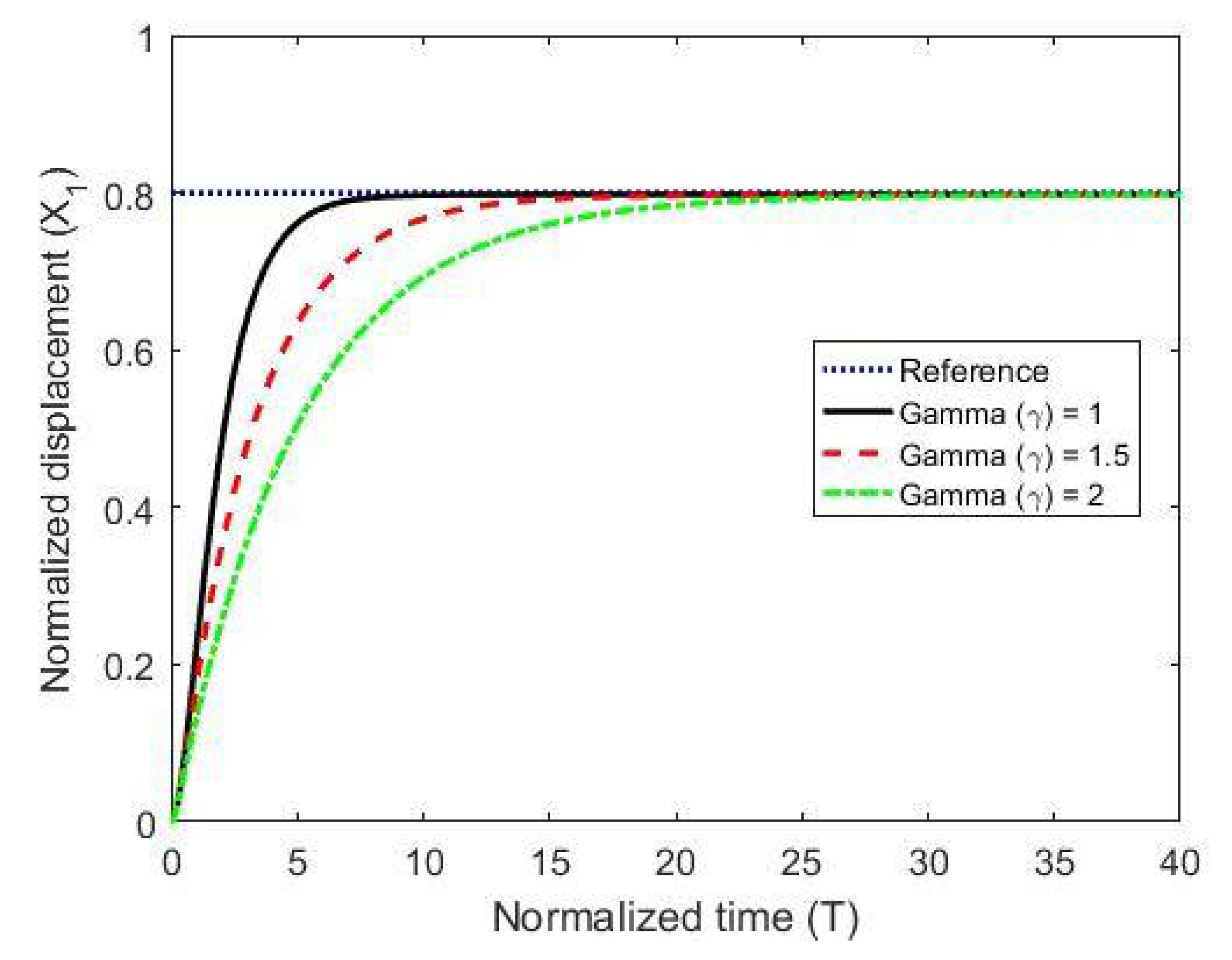
5.1. Simulations Using MATLAB/Simulink environment

To test the proposed controller, we built a numerical model using the MATLAB/Simulink environment and using normalized expressions. In these simulations, we chose the damping ratio ζ = 0.5, the natural frequency ${\omega }_n=1$, and the controller constants (gains) as $K_1=10, K_v=10, k_2=5$ and $K_i=0.003$. The results are shown in Figure 3, Figure 4 and Figure 5 for different reference signals and for a coupling term $\gamma =1.$ To show the advantage of the proposed controller, the results are compared to the same model without the coupling constant, i.e., $\gamma =0$.

The figures demonstrate that both controllers stabilize the system throughout the full gap distance, i.e., beyond the pull-in range. Also, the coupling improves the response by reducing the overshoot for a step response. The estimated speed is shown in Figure 6, Figure 7 and Figure 8 for different reference signals and for $\gamma =1.$

The results for stabilization of the plate by varying the coupling term ($\gamma$) are shown in Figure 9.

Finally, to show the advantage and robustness of this method even if the system has a lighter damping factor, the closed-loop system has been simulated with a damping factor of ζ = 0.01 as shown in Figure 10, Figure 11 and Figure 12.

The figures show that without coupling the system suffers from oscillation and overshoot above its normalized limit ($x_1=1$). The transient behavior of the system has been significantly improved by introducing the coupling, which demonstrates the effectiveness of the proposed controller.

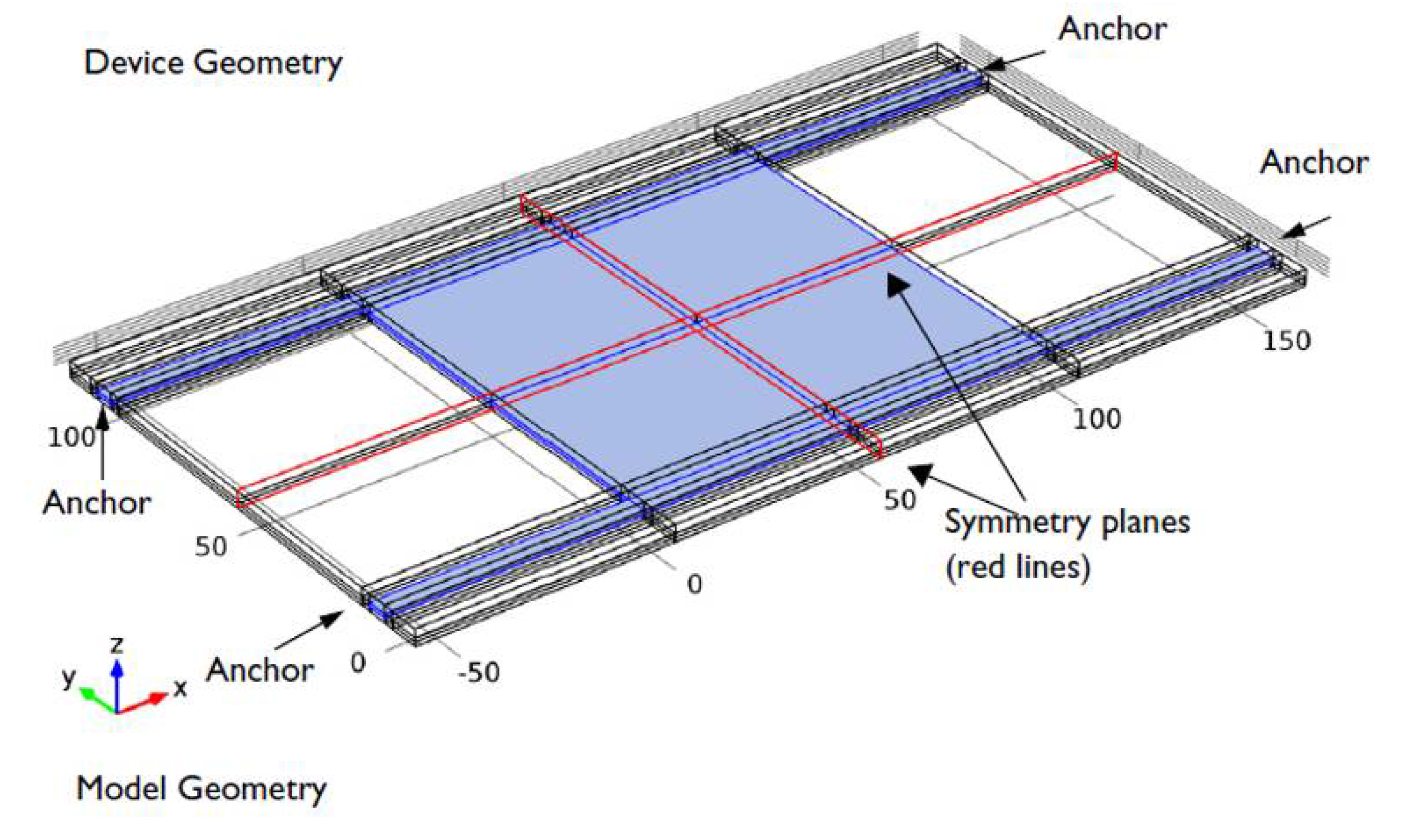
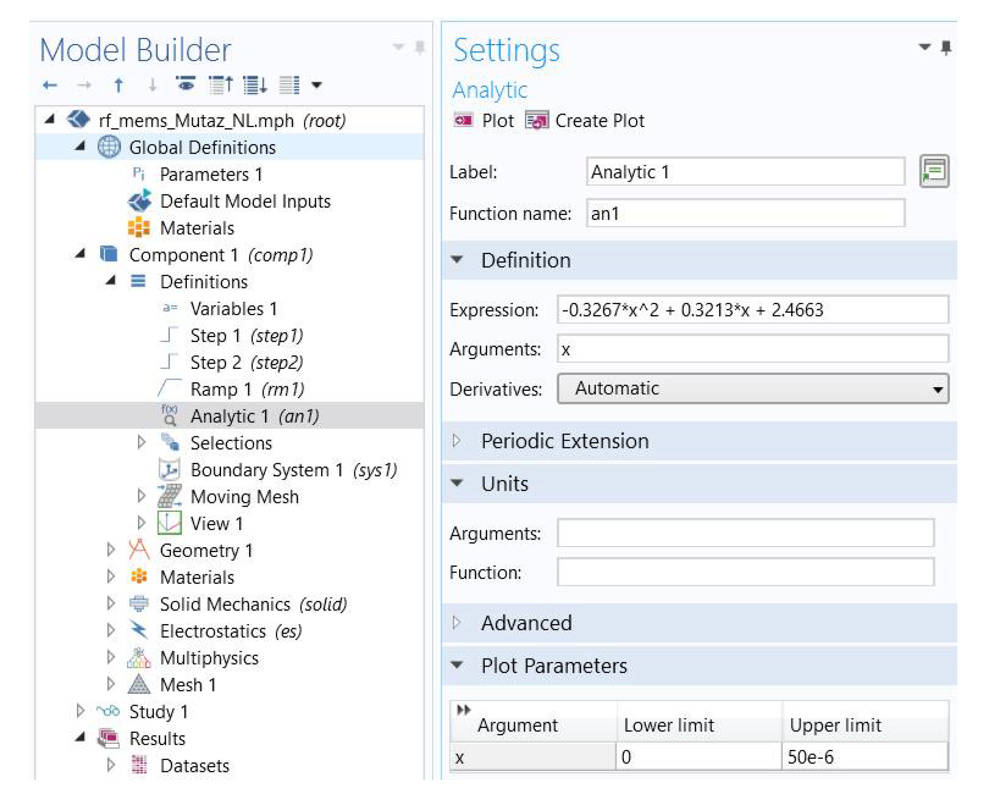
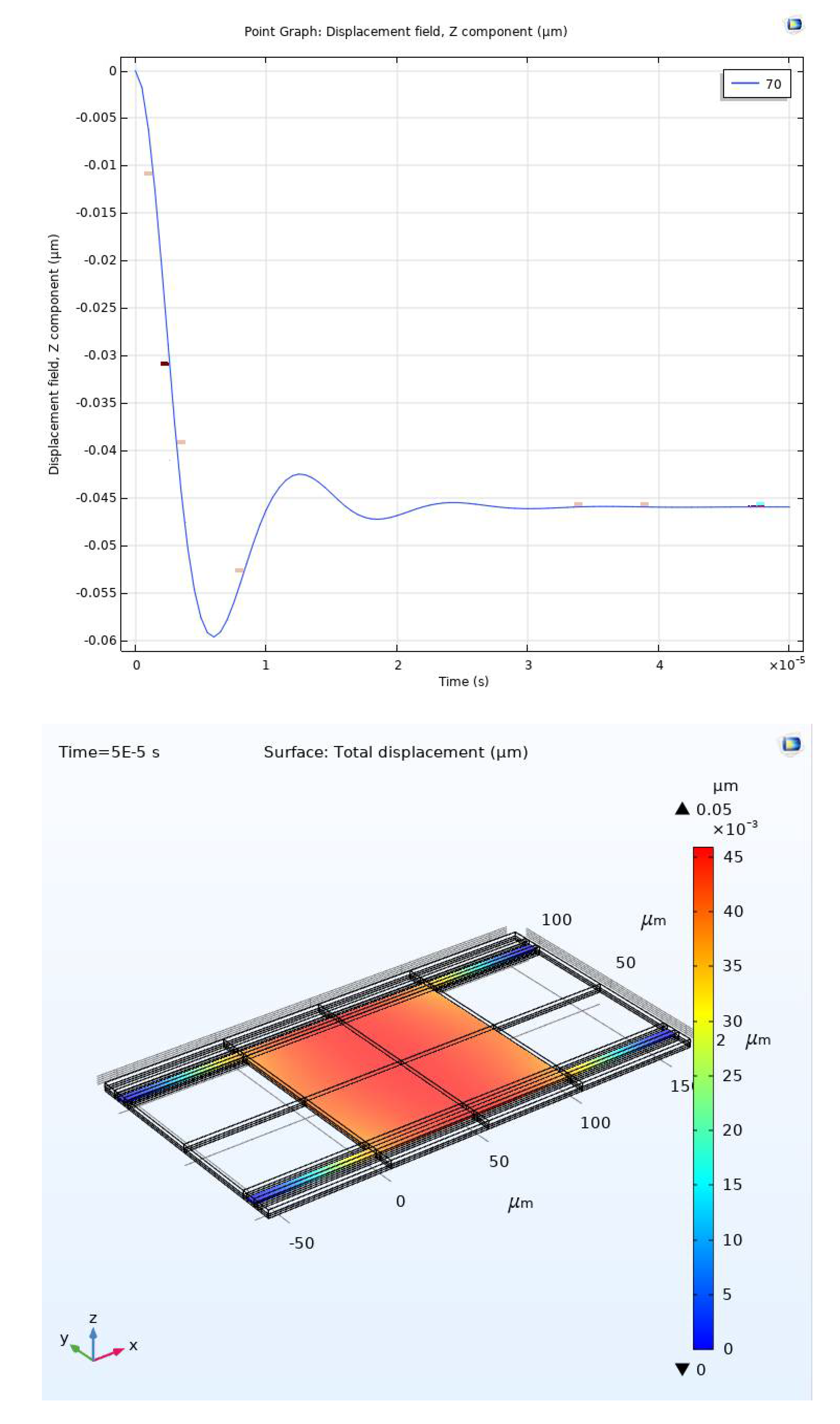
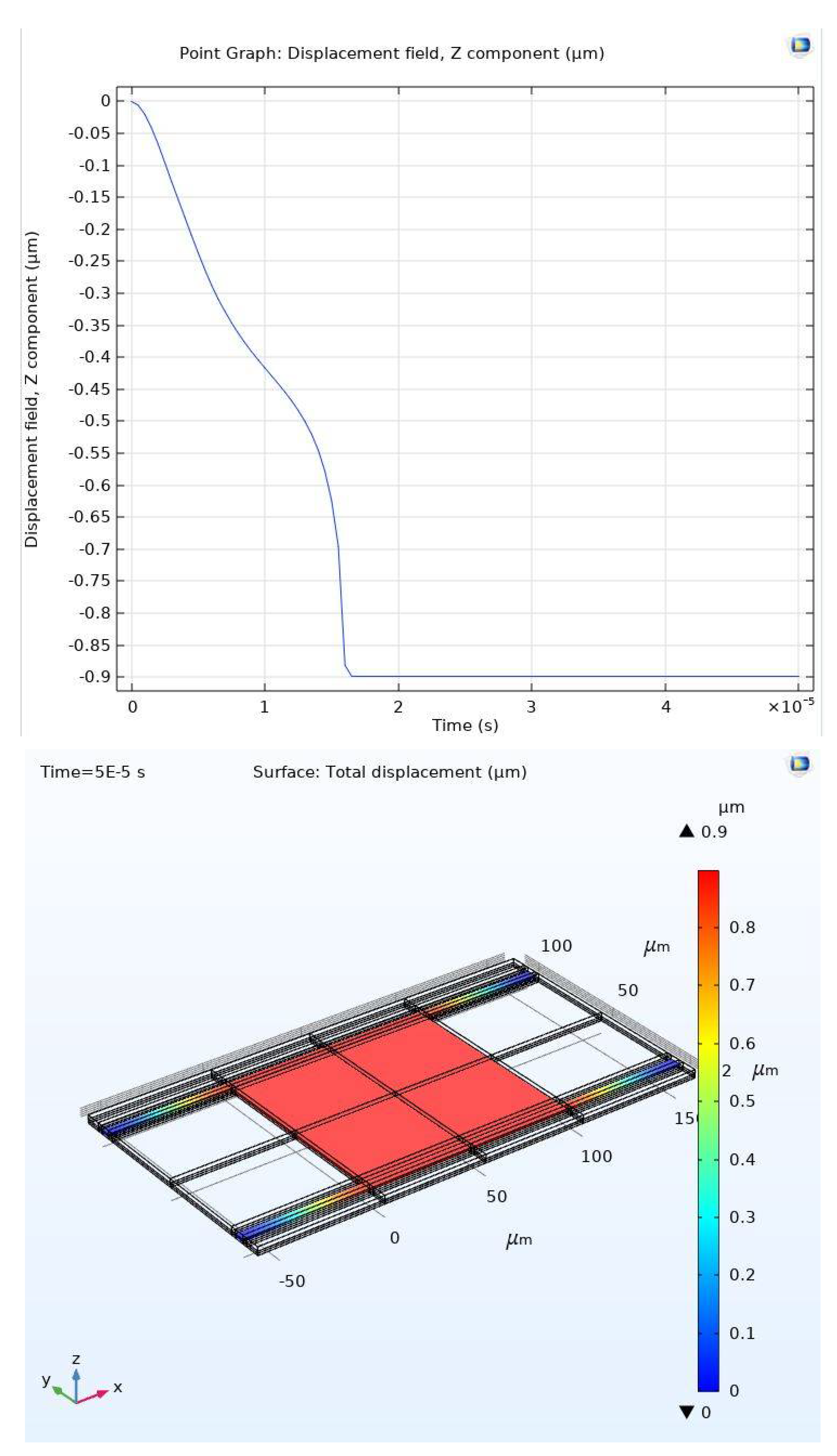
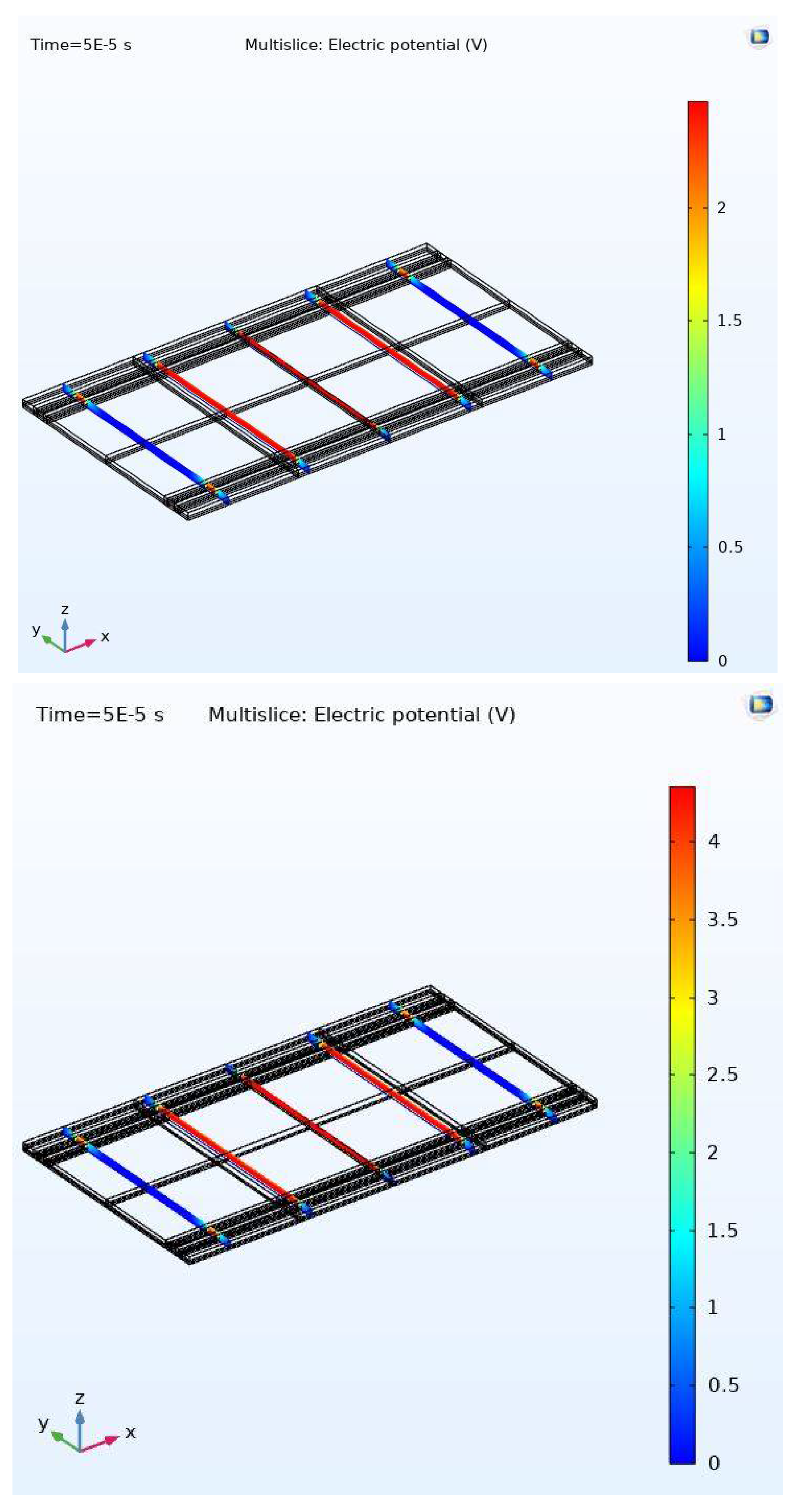
5.2. Simulations Using Multiphysics Modelling Software COMSOL

The results have also been demonstrated with numerical simulations on the RF MEMS device using COMSOL software. We use the model example of [34] to illustrate our simulation results. The schematic view of the RF MEMS device is shown in Figure 13. The device consists of square parallel plates (electrodes), one grounded (fixed) and one movable plate formed from polysilicon and suspended 0.9 $\mathsf{\mu }$m above a 0.1 $\mathsf{\mu }$m thick dielectric layer of silicon nitride. The device is actuated electrostatically by applying a voltage signal. The parameters of the model are the same as in [34], and are repeated here in

Table 1. Parameters of the RF MEMS device.

Parameter	Value
Plate length	L = 50 μm
Plate thickness	t = 2 μm
Gap between the plates	$q_z=1.1 \mathsf{\mu }\mathrm{m}=1.1 \mathsf{\mu }\mathrm{m}$
Permittivity	$ϵ=4.5={4.5}^{°}$
Density	$\rho =2320 \mathrm{kg}/{\mathrm{m}}^3/{\mathrm{m}}^3$
Damping ratio	ζ = 1 × ${10}^{-6}$
Spring stiffness	k = 128 N/m

for ease of reference:

For the sake of controller design aiming at producing the voltage input, the RF model has been first simulated in the MATLAB/Simulink environment. We used the “simout” function, which allows the definition of a voltage signal as an expression from a set of points either with linear interpolation (best fit line) or as a polynomial formula. This formula is introduced to the COMSOL model as depicted in Figure 14.

Figure 15 and Figure 16 show the simulation results for the RF MEMS device using COMSOL software. Simulation results are obtained for displacements through the gap (0–1.01 $\mathsf{\mu }\mathrm{m})$. Figure 15 shows the stabilization of the upper (movable) plate at the first one-third of the gap at 0.046 $\mathsf{\mu }\mathrm{m}$.

Figure 16 shows the stabilization of the movable plate at 0.9 $\mathsf{\mu }\mathrm{m}$ which is in the last third of the full gap, i.e., beyond the pull-in instability range. Thus, the effectiveness of the proposed controller is demonstrated by two sets of simulations, which both showed successful stabilizing of the electrostatically MEMS device through the full range with improved performance.

Finally, Figure 17 shows the voltage (electric potential (V)) as the control input that actuates the RF MEMS device and moves the upper plate in the $z$ coordinate towards the fixed plate (for the 2 positions above). As expected from the theory, a higher voltage signal (around 4.5 V) was needed to move the plate to the 0.9 $\mathsf{\mu }\mathrm{m}$ position (near the fixed plate) compared to around 2.5 V that was needed to stabilize the movable plate at 0.046 $\mathsf{\mu }\mathrm{m}$ (i.e., in the first-third of gap).

6. Conclusions

In this paper, the IDA-PBC method was used to design a dynamic controller for stabilization and improving the performance of an electrostatic MEMS actuator across the full gap distance. An improved response was obtained by utilizing coordinate transformations and forcing a coupling between the electric charge and the momentum in the interconnection matrix. A speed observer was also employed to estimate the speed (momentum), which is hard to measure in real applications. Simulation results of the electrostatic MEMS actuator suitably verified the proposed dynamic IDA-PBC controller and the speed observer. The validation of the proposed control design method was obtained using two simulation environments, namely: MATLAB/Simulink and COMSOL Multiphysics.

References

1. Zhang, W.-M.; Yan, H.; Peng, Z.-K.; Meng, G. Electrostatic pull-in instability in MEMS/NEMS: A review. Sens. Actuators A Phys. 2014, 214, 187–218. [Google Scholar] [CrossRef]
2. Agudelo, C.G.; Packirisamy, M.; Zhu, G.; Saydy, L. Nonlinear Control of an Electrostatic Micromirror Beyond Pull-In with Experimental Validation. J. Microelectromech. Syst. 2009, 18, 914–923. [Google Scholar] [CrossRef]
3. Oh, K.W.; Ahn, C.H. A review of microvalves. J. Micromech. Microeng. 2006, 16, 13–39. [Google Scholar] [CrossRef]
4. Uhlig, S.; Gaudet, M.; Langa, S.; Schimmanz, K.; Conrad, H.; Kaiser, B.; Schenk, H. Electrostatically Driven In-Plane Silicon Micropump for Modular Configuration. Micromachines 2018, 9, 190. [Google Scholar] [CrossRef] [PubMed] [Green Version]
5. Maithripala, D.H.S.; Berg, J.M.; Dayawansa, W.P. Control of an Electrostatic Microelectromechanical System Using Static and Dynamic Output Feedback. J. Dyn. Syst. Meas. Control 2005, 127, 443–450. [Google Scholar] [CrossRef]
6. Dong, L.; Edwards, J. Active Disturbance Rejection Control for an Electro-Statically Acuated MEMS Device. Int. J. Intell. Control Syst. 2011, 16, 160–169. [Google Scholar]
7. Karkoub, M.; Zribi, M. Robust Control of an Electrostatic Microelectromechanical Actuator. Open Mech. J. 2008, 2, 12–20. [Google Scholar] [CrossRef]
8. Zhu, G.; Levine, J.; Praly, L. Stabilization of an electrostatic MEMS including uncontrollable linearization. In Proceedings of the 46th IEEE Conference on Decision and Control, New Orleans, LA, USA, 12–14 December 2007; pp. 2433–2438. [Google Scholar]
9. Salah, M.H.; Alwidyan, K.M.; Tatlicioglu, E.; Dawson, D. Robust Backstepping Nonlinear Control for Parallel-Plate Micro Electrostatic Actuators. In Proceedings of the 49th IEEE Conference on Decision and Control (CDC), Atlanta, GA, USA, 15–17 December 2010. [Google Scholar]
10. Zhu, G.; Lévine, J.; Praly, L. Improving the performance of an electrostatically actuated MEMS by nonlinear control: Some advances and comparisons. In Proceedings of the 44th IEEE CDC ECC, Seville, Spain, 12–15 December 2005; pp. 7534–7539. [Google Scholar]
11. Wickramasinghe, I.P.M.; Maithripala DH, S.; Kawade, B.D.; Berg, J.M.; Dayawansa, W.P. Passivity-Based Stabilization of a 1-DOF Electrostatic MEMS Model With a Parasitic Capacitance. IEEE Trans. Control Syst. Technol. 2009, 17, 249–256. [Google Scholar] [CrossRef]
12. Dong, X.; Yang, S.; Zhu, J.; En, Y.; Huang, Y. Method of Measuring the Mismatch of Parasitic 0ance in MEMS Accelerometer Based on Regulating Electrostatic Stiffness. Micromachines 2018, 9, 128. [Google Scholar] [CrossRef] [PubMed] [Green Version]
13. Iqbal, F.; Lee, B. A Study on Measurement Variations in Resonant Characteristics of Electrostatically Actuated MEMS Resonators. Micromachines 2018, 9, 173. [Google Scholar] [CrossRef] [PubMed] [Green Version]
14. Feng, J.; Liu Ch Zhang, W.; Hao, S. Static and Dynamic Mechanical Behaviors of Electrostatic MEMS Resonator with Surface Processing Error. Micromachines 2018, 9, 34. [Google Scholar] [CrossRef] [PubMed] [Green Version]
15. Newton, B. Design of Curved Electrodes to Enable Large Stroke—Low Voltage Micro Actuators. Ph.D. Thesis, Massachusetts Institute of Technology, Cambridge, MA, USA, 2016. [Google Scholar]
16. Preetham, B.S.; Hoelzle, D.J. Experimental investigation of curved electrode actuator dynamics in viscous dielectric media. Appl. Phys. Lett. 2018, 113, 074102. [Google Scholar]
17. Preetham, B.S.; Lake, M.A.; Hoelzle, D.J. A curved electrode electrostatic actuator designed for large displacement and force in an underwater environment. J. Micromech. Microeng. 2017, 27, 095009. [Google Scholar] [CrossRef]
18. Petrov, D.; Lang, W.; Benecke, W. A nickel electrostatic curved beam actuator for valve applications. Procedia Eng. 2010, 5, 1409–1412. [Google Scholar] [CrossRef] [Green Version]
19. Ortega, R.; van der Schaft, A.J.; Maschke, B.; Escobar, G. Interconnection and damping assignment passivity-based control of port-controlled Hamiltonian systems. Automatica 2002, 38, 585–596. [Google Scholar] [CrossRef] [Green Version]
20. Yuksel, B.; Secchi, C.; Bülthoff, H.; Hand Franchi, A. Reshaping the physical properties of a quadrotor through IDA-PBC and its application to aerial physical interaction. In Proceedings of the 2014 IEEE Int. Conference on Robotics and Automation, Hong Kong, China, 31 May–7 June 2014; pp. 6258–6265. [Google Scholar]
21. Ryalat, M. Design and Implementation of Nonlinear and Robust Control for Hamiltonian Systems: The Passivity-Based Control Approach. Ph.D. Thesis, University of Southampton, Southampton, UK, 2015. [Google Scholar]
22. Gaviria, C.; Fossas, E.; Griñó, R. Robust Controller for a Full-Bridge Rectifier Using the IDA Approach and GSSA Modeling. IEEE Trans. Circuits Syst. 2005, 52, 609–616. [Google Scholar] [CrossRef] [Green Version]
23. Garcia-Tenorio, C.; Quijano, N.; Mojica-Nava, E.; Sofrony, J. Bond Graph Model-Based for IDA-PBC. In Proceedings of the 2016 IEEE Conference on Control Applications (CCA) Part of 2016 IEEE Multi-Conference on Systems and Control, Buenos Aires, Argentina, 19–22 September 2016; pp. 1098–1103. [Google Scholar]
24. Ryalat, M.; Laila, D.S.; Almtireen, N.; ElMoaqet, H. A Novel Dynamic IDA-PBC Controller for Electrostatic MEMS Devices. In Proceedings of the 2018 Annual American Control Conference (ACC), Milwaukee, WI, USA, 27–29 June 2018; pp. 2952–2957. [Google Scholar]
25. Ryalat, M.; Laila, D.; ElMoaqet, H.; Almtireen, N. Dynamic IDA-PBC Control for Weakly-Coupled Electromechanical Systems. Automatica 2020, 115, 108880. [Google Scholar] [CrossRef]
26. Crespo, M.; Donaire, A.; Ruggiero, F.; Lippiello, V.; Siciliano, B. Design, Implementation and Experiments of A Robust Passivity-Based Controller for A Rolling-Balancing System. In Proceedings of the 13th International Conference on Informatics in Control, Automation and Robotics, Lisbon, Portugal, 29–31 July 2016; pp. 79–89. [Google Scholar]
27. Donaire, A.; Junco, S. On the addition of integral action to port-controlled Hamiltonian systems. Automatica 2009, 45, 1910–1916. [Google Scholar] [CrossRef]
28. Nemirovsky, Y.; Bochobza-Degani, O. A methodology and model for the pull-in parameters of electrostatic actuators. J. Microelectromech. Syst. 2001, 10, 601–615. [Google Scholar] [CrossRef] [Green Version]
29. Rodriguez, H.; Ortega, R. Stabilization of electromechanical systems via interconnection and damping assignment. Int. J. Robust Nonlinear Control 2003, 13, 1095–1111. [Google Scholar] [CrossRef]
30. Maithripala DH, S.; Berg, J.M.; Dayawansa, W.P. Capacitive stabilization of an electrostatic actuator: Output feedback viewpoint. In Proceedings of the 2003 American Control Conference, Denver, CO, USA, 4–6 June 2003; pp. 4053–4058. [Google Scholar]
31. Senturia, S. Microsystem Design; Kluwer: Norwell, MA, USA, 2001. [Google Scholar]
32. Khalil, H. Nonlinear Systems, 3rd ed.; Prentice Hall: Upper Saddle River, NJ, USA, 2002. [Google Scholar]
33. Van der Schaft, A.J. L2-Gain and Passivity Techniques in Nonlinear Control; Springer: Berlin/Heidelberg, Germany, 2000. [Google Scholar]
34. COMSOL: Application Gallery, “Pull-In of an RF MEMS Switch”. Available online: https://www.comsol.com/model/pull-in-of-an-rf-mems-switch-16379 (accessed on 11 July 2020).
Figure 1. Scheme of 1-DOF parallel-plate electrostatic actuator.
Micromachines 11 00688 g001
Figure 2. Pull-in displacement characteristic of the microactuator.
Micromachines 11 00688 g002
Figure 3. The normalized displacement with and without the coupling constant at a gap distance of 0.3.
Micromachines 11 00688 g003
Figure 4. The normalized displacement with and without the coupling constant at a gap distance of 0.5.
Micromachines 11 00688 g004
Figure 5. The normalized displacement with and without the coupling constant at a gap distance of 0.8.
Micromachines 11 00688 g005
Figure 6. The normalized estimated velocity with the coupling constant at a gap distance of 0.3.
Micromachines 11 00688 g006
Figure 7. The normalized estimated velocity with the coupling constant at a gap distance of 0.5.
Micromachines 11 00688 g007
Figure 8. The normalized estimated velocity with the coupling constant at a gap distance of 0.8.
Micromachines 11 00688 g008
Figure 9. The normalized displacement with a different coupling term at a gap reference of 0.8.
Micromachines 11 00688 g009
Figure 10. The normalized displacement with and without the coupling constant at a gap distance of 0.8 and damping ratio ζ = 0.01.
Micromachines 11 00688 g010
Figure 11. The normalized estimated velocity with the coupling constant at a gap distance of 0.8 and damping ratio ζ = 0.01.
Micromachines 11 00688 g011
Figure 12. The normalized displacement with different coupling terms at a gap reference of 0.8 and damping ratio ζ = 0.01.
Micromachines 11 00688 g012
Figure 13. Schematic view of the RF MEMS device.
Micromachines 11 00688 g013
Figure 14. Model configuration and setting on COMSOL.
Micromachines 11 00688 g014
Figure 15. Stabilization at the first third of the full gap: top graph (1-D), bottom graph (3-D).
Micromachines 11 00688 g015
Figure 16. Stabilization at the last third of the full gap: top graph (1-D), bottom graph (3-D).
Micromachines 11 00688 g016
Figure 17. Control input (voltage) at two positions: top graph (0.046 μ m ), bottom graph (0.9 μ m ).
Micromachines 11 00688 g017