Glacier Remote Sensing Using Sentinel-2. Part II: Mapping Glacier Extents and Surface Facies, and Comparison to Landsat 8

Abstract

Mapping of glacier extents from automated classification of optical satellite images has become a major application of the freely available images from Landsat. A widely applied method is based on segmented ratio images from a red and shortwave infrared band. With the now available data from Sentinel-2 (S2) and Landsat 8 (L8) there is high potential to further extend the existing time series (starting with Landsat 4/5 in 1982) and to considerably improve over previous capabilities, thanks to increased spatial resolution and dynamic range, a wider swath width and more frequent coverage. Here, we test and compare a variety of previously used methods to map glacier extents from S2 and L8, and investigate the mapping of snow facies with S2 using top of atmosphere reflectance. Our results confirm that the band ratio method works well with S2 and L8. The 15 m panchromatic band of L8 can be used instead of the red band, resulting in glacier extents similar to S2 (0.7% larger for 155 glaciers). On the other hand, extents derived from the 30 m bands are 4%–5% larger, indicating a more generous interpretation of mixed pixels. Mapping of snow cover with S2 provided accurate results, but the required topographic correction would benefit from a better orthorectification with a more precise DEM than currently used.

1. Introduction

Glacier mapping is a key application of optical satellite data and has been widely applied, in particular after the Landsat image archives were opened to the public and offering orthorectified (i.e., terrain corrected) products [1]. As glacier changes are key indicators of climate change [2] and their outlines are mandatory for any glacier-specific calculations and modeling (e.g., length, volume/mass changes, run-off, ice thickness, and future glacier development), there was a high demand for a globally complete glacier inventory. The now available Randolph Glacier Inventory (RGI) has finally been accomplished, thanks to the freely available Landsat images and a special community effort [3]. Glacier classification is based on the strong difference in spectral reflectance of snow and glacier ice in the visible and near infrared (VNIR) compared to the shortwave infrared (SWIR). Whereas snow and ice have a high absorption in the SWIR, ice and in particular snow have a high reflectance in the VNIR [4]. By dividing the raw digital numbers (DNs) of a VNIR band by those from the SWIR, illumination effects due to topography are minimized and glaciers stand out bright against a dark background. With a simple threshold, the ratio image is transformed to a glacier map (clean ice only) and corresponding glacier outlines [5]. Simple band ratios have proven to be fast, robust (results are insensitive to the thresholds) and accurate compared to other, often more complex and computationally intensive methods [6,7] or reference datasets [8]. The method has thus been widely applied for large-scale glacier mapping with Landsat data in many regions of the world [9,10,11,12,13]. Owing to their spectral similarity with the surrounding terrain, however, debris-covered glacier parts cannot be mapped from spectral properties alone. Accordingly, a wide range of combined methods has been developed to identify debris-covered glacier parts [14,15,16,17].

With the Landsat Thematic Mapper (TM) sensor being decommissioned after 27 years of operation in 2012, ETM+ suffering from a malfunction of its scan-line corrector, and ASTER being near the end of its life time (its SWIR band failed in 2009), the chances for repeated glacier mapping on a larger regional scale were increasingly challenged. However, with the successful launch of Landsat 8 on 11 February 2013 and its improved sensor Operational Land Imager (OLI), as well as the launch of Sentinel-2A (S2A) on 23 June 2015 operating the new Multi Spectral Instrument (MSI), glacier mapping and change assessment can be continued after a one-year gap in 2012. Thereby, the higher spatial resolution of S2A compared to Landsat (10 m instead of 30 m) and its shortened repeat interval (10 days with S2A, and five days with S2A and S2B in orbit) will help reducing two major problems: debris-covered glaciers can be delineated more precisely and the chance to acquire cloud-free images at the end of the ablation period (or dry season) with a minimum snow extent increases. Both MSI and OLI provide additional spectral bands, have adjusted spectral ranges, and a higher dynamic range (12 bit instead of 8 bit) than the previous Landsat sensors.

Due to these new capabilities, this Part II of the joint study on Sentinel-2A investigates whether the methods for glacier and snow facies mapping developed for previous sensors (band ratios) can still be applied, how the results compare between the two sensors OLI and MSI, and if their data can be used to continue the available time series for glacier monitoring. For the analysis of the radiometric and geometric performance of Sentinel-2A, we refer to Part I of this joint study [18]. This Part II of the study has the following three major aims:

(1)

testing various spectral band combinations for mapping glaciers from raw DNs;

(2)

comparison of glacier outlines derived from OLI and MSI using raw DNs;

(3)

mapping bare ice and snow using top of atmosphere reflectance (TOAR) from MSI.

The first test (1) has a focus on threshold sensitivity; the second (2) on the impacts of different spatial resolutions and band combinations; and the third (3) on the impacts of DEM resolution (a DEM has to correct terrain-related illumination differences). For (1) and (2), we compare the derived glacier outlines and areas for the thresholds used and highlight the problematic issues. For (2), we here also analyze for the first time the use of the 15 m resolution OLI panchromatic band (OLI 8) instead of the 30 m red band (OLI 4) to obtain a higher resolution product from Landsat and compare it to both the red/SWIR ratio with 30 m and the MSI ratio with 10 m resolution. For (3), the threshold-based method developed by [19] has been adapted for the MSI sensor to retrieve information on snow and ice areas on glaciers. Under some constraints, the snow areas can be used as a proxy for glacier mass balance [20,21] and might be useful for hydrologic applications [22].

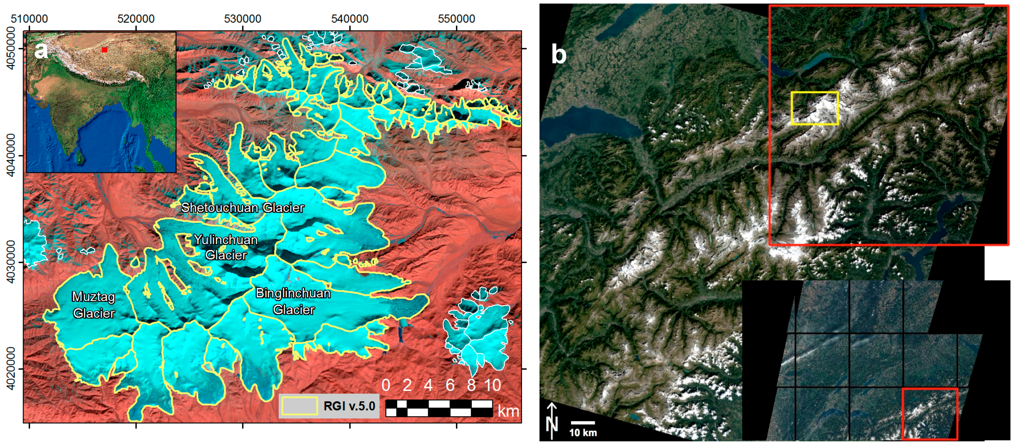
2. Study Regions and Datasets

We exemplify each of the above three comparisons in three dedicated test regions (see Figure 1 for two of them): the Kunlun Mountains in northern Tibet is region 1, the Lauterbrunnen Valley in the Swiss Alps is region 2, and the Venediger Mountains in the Austrian Alps (Hohe Tauern) is region 3. Whereas the two Alpine test regions 2 and 3 are located along the northern main ridge of the Alps and experience more maritime climate conditions (annual precipitation around 2–3 m with high spatial variability [23]), test region 1 is an isolated mountain group in a dry continental climate (annual precipitation about 0.5 m [24]) where glaciers are losing mass also by sublimation. The latter can result in rough and chaotic ablation regions, but overall they have little debris cover and can thus be mapped automatically with the band ratio method. The highest mountain in this region is Ulugh Muztagh (6973 m) and glaciers stretch down to 5100 m. In the two alpine test sites, glaciers stretch from about 4000 m (Jungfrau: 4160 m, Großvenediger: 3670 m) down to 2200 m.

Both alpine regions have steep rock walls casting shadow on glaciers and were selected for this reason, as shadow regions are most sensitive to small changes of the threshold for the ratio images. In test region 1, the occurrence of thin snow is also on purpose to analyze the threshold sensitivity.

Whereas test region 1 has mostly debris free glaciers, some seasonal snow and is based on version 2.0 of Sentinel-2A data (with a re-scaled 12-bit range from 1 to 10,000) [25], test region 2 has many heavily debris-covered glaciers, virtually no seasonal snow off glaciers and is based on S2A data acquired on 29 August 2015 during the commissioning phase (v1.0) with scaled radiances between 1 and 1000. The OLI image for the same region (path-row: 195-028) was acquired only 2 days later (31 August 2015) and is based on the USGS standard L1T processing. Test region 3 includes mostly debris-free glaciers and is covered by a v1.0 S2A scene acquired during the commissioning phase on 13 August 2015. It has a strong reflectance differences between snow and bare ice on glaciers but still some seasonal snow left off-glaciers.

Table 1. Characteristics of the scenes used for the three test regions.

Test Site	Satellite	Sensor	MSI Tile or Path-Row	Date	Region	Product	Quantization
1	Sentinel 2A	MSI	T45SWA	18 November 2015	Tibet	Ramp-up Phase	1–10,000
2	Sentinel 2A	MSI	T32TMS	29 August 2015	Alps (CH)	Commissioning Phase	1–1000
2	Landsat 8	OLI	195-028	31 August 2015	Alps (CH)	USGS L1T	16 bit
3	Sentinel 2A	MSI	T32TQT	13 August 2015	Alps (AT)	Commissioning Phase	1–1000

provides summary information for all selected satellite scenes.

In Figure 2 we present a close up of test region 2 (see location in Figure 1) for a direct comparison of a few glaciers as seen with 10 m (MSI) and 30 m (OLI) spatial resolution in natural colors. Obviously, debris-covered parts (in the upper center) or crevasses (near the lower center) that are important to identify the nature of a glacier are much better visible at 10 m resolution. The two scenes from MSI and OLI were acquired in the last week of August and have less seasonal snow and are thus better suited for glacier mapping. As snow conditions were getting unsuitable for glacier mapping after 1 September 2015, acquisition of cloud free images with the best snow conditions for glacier mapping was only possible within this one week. The future high repeat frequency of MSI is thus most welcome.

Additional to the satellite scenes we used in region 2, a vector layer with drainage divides obtained in a previous study from the SRTM DEM [26] to determine glacier-specific areas for a direct comparison of mapping results among the different sensors. The pre-processing of the MSI scene for mapping glacier facies in region 3 requires a DEM. However, the DEM used for the orthorectification was not available for this study and different national and global DEMs with pixel sizes ranging from 10 to 90 m were resampled to 10 m and tested for the MSI pre-processing. We finally selected a resampled ASTER GDEM v2 for processing.

3. Methods

3.1. Sensor Characteristics

The spectral ranges and spatial resolution of the three Landsat sensors TM, ETM+ and OLI are listed in

Table 2. Spectral band ranges of the optical sensors that are used for glacier mapping. The spatial resolution (in m) is color-coded: 10 ($\text{green}$), 15 ($\text{blue}$), 20 ($\text{red}$), and 30 (black). NIR: near infrared, SWIR: shortwave infrared, Pan: panchromatic. Sources: [27,28,29].

	Band Number					Landsat			Sentinel-2A	Terra
Band	TM	ETM+	OLI	MSI	AST	TM	ETM+	OLI	MSI	ASTER
Blue	1	1	2	2	-	0.45–0.52	0.45–0.52	0.45–0.51	$0.46–0.52$	-
Green	2	2	3	3	1	0.52–0.60	0.53–0.61	0.53–0.60	$0.54–0.58$	$0.52–0.60$
Red	3	3	4	4	2	0.63–0.69	0.63–0.69	0.63–0.68	$0.65–0.68$	$0.63–0.69$
NIR	4	4	5	8	3	0.76–0.90	0.76–0.90	0.85–0.89	$0.78–0.90$	$0.76–0.86$
SWIR	5	5	6	11	4	1.55–1.75	1.55–1.75	1.56–1.66	$1.57–1.66$	1.60–1.70
SWIR	7	7	7	12	5–9	2.08–2.35	2.09–2.35	2.10–2.30	$2.10–2.28$	2.15–2.43
Pan	-	8	8	-	-	-	$0.52–0.90$	$0.50–0.68$	-	-

along with the equivalent bands of the Sentinel-2A MSI and for reference also the Terra ASTER sensor (cf. Figure 1 in Part I of this paper). The panchromatic band with 15 m resolution is only available on ETM+ and OLI, and ASTER does not have a band in the blue part of the spectrum. The spectral range covered by the OLI panchromatic band is decreased considerably: it covered the green, red and NIR band on ETM+, but on OLI it now covers the green, red and a small part of the blue bands. As the green and red bands have been successfully applied in glacier mapping, we test here if the higher resolution panchromatic band can also be used for this. As for the MSI sensor, this requires resampling the SWIR band to match the resolution of the respective other band (from 30 to 15 m for OLI and from 20 m to 10 m for MSI). In general, the spectral bandwidth of most MSI bands is smaller than for the respective Landsat and ASTER sensors.

Glaciers are usually classified from spectral band ratios and one or two thresholds can be applied to the ratio (abbreviated in the following with th1) and/or single bands (th2). As an input, either raw digital numbers (DNs) or converted values (e.g., spectral reflectance, TOAR) are used. For this study, two versions of calibrated reflectances are used for MSI and raw DNs for OLI (Table 1). Whereas the glacier mapping in region 1 used reflectance values between 1 and 10,000 (v2.0), the previous scaling between 1 and 1000 (v1.0) was used for regions 2 and 3. This rescaling does not change the spectral characteristics, because the radiance information in each pixel is kept. The histograms of the two processing versions have thus a similar distribution of values before and after the scaling. In effect, the threshold value (th1) for the ratio does not change much due to the different scaling; however, the MSI band 2 threshold (th2) changes by approximately an order of magnitude, for example from 110 in test region 2 to 1100 in region 1.

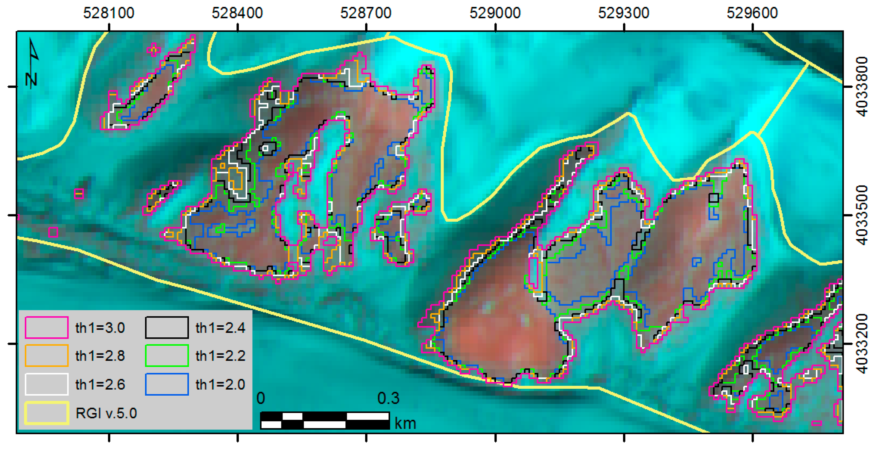
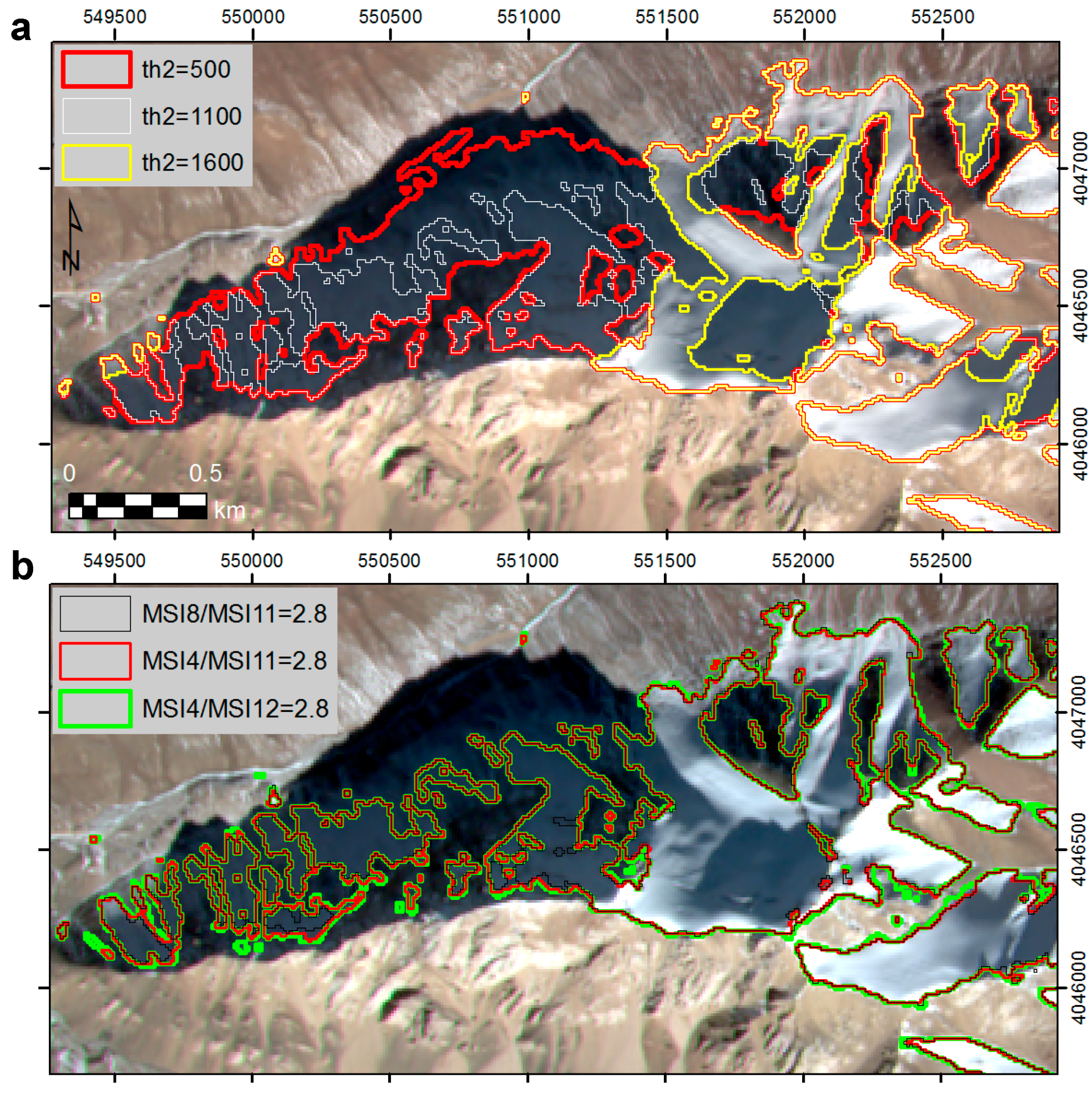
3.2. Analysing Band Ratios and Thresholds in Test Region 1 (Northern Tibet)

As a first test of glacier mapping with MSI we applied some of the band ratios used in previous studies with Landsat TM and ETM+ and tested the impact of various thresholds on the mapped glacier area. The Normalized Difference Snow Index (NDSI) has also been tested but results are not shown here, as they were less favorable than the simple band ratios, at least when used without applying a simple atmospheric correction [5,7]. The ratios tested are:

(a)

the red/SWIR ratio (MSI4/MSI11) with an additional threshold in the blue band (MSI2) for improved classification of ice in shadow [7];

(b)

the red/SWIR ratio (MSI4/MSI12) using the second SWIR band (center wavelength 2.19 μm);

(c)

the NIR/SWIR ratio (MSI8/MSI11) [5,30].

For (a), (b) and (c), thresholds are changed in steps of 0.2 (from 2.0 to 3.0) for the ratio and—only for (a)—in steps of 100 (from 500 to 2000) for MSI2. The choices of threshold values are in agreement with previous studies [5,8,31]. For all band ratios visual inspection was used to select an empirical threshold value. Band ratio results are smoothed with a median filter (3 by 3 kernel size) before conversion of the binary glacier maps to vector files. To calculate the ratios, the SWIR band was resampled from 20 to 10 m using a simple bilinear interpolation to capture all information available in both bands. Glacier outlines from the RGI were used for a qualitative comparison, but do not allow a quantitative validation due to the temporal difference of about 5 years.

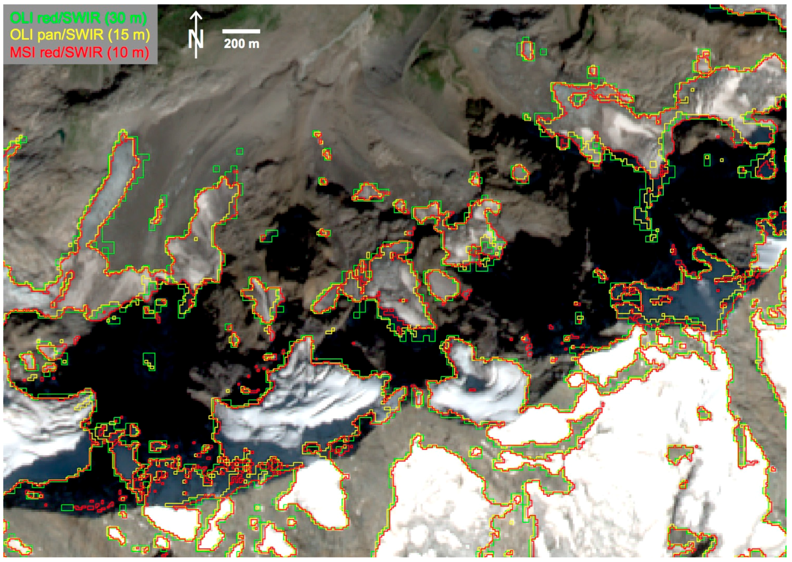
3.3. Glacier Mapping in Test Region 2 (Swiss Alps)

For test region 2 (Jungfrau region), clean ice and snow were mapped with the simple band ratio method using the raw values from the respective bands of OLI and MSI. In all cases, the thresholds th1 and th2 were selected manually and optimized by visual control on the original image by overlay of the resulting outlines. Overall, three different ratios were applied and analyzed:

(d)

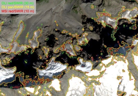
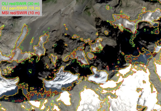
the red/SWIR band ratio at 30 m resolution: OLI4/OLI6 > th1;

(e)

a new band ratio with the 15 m panchromatic band: OLI8/OLI6 > th1;

(f)

for Sentinel-2A, a 10 m resolution dataset from the ratio MSI4/MSI11 > th1 and MSI2 > th2.

In cases (e) and (f), the SWIR bands of OLI6 and MSI11 were resampled beforehand to 15 m and 10 m resolution, respectively, using bilinear interpolation. To improve classification accuracy with MSI, it was required to exclude bare rock in shadow with an additional (manually selected) threshold th2 on MSI band 2 as for (a) in test region 1. A smoothing median filter was not applied to the resulting glacier masks to determine mapping accuracy also in regard to fine spatial details. We compared the obtained mapping results visually (by overlay of outlines) and quantitatively by calculating the mapped areas for 155 glaciers (after digital intersection with drainage divides) from all three methods (d) to (f). Due to the variability in the mapped extents (attached and separated glacier parts), area values were extracted manually for each individual glacier in each vector layer.

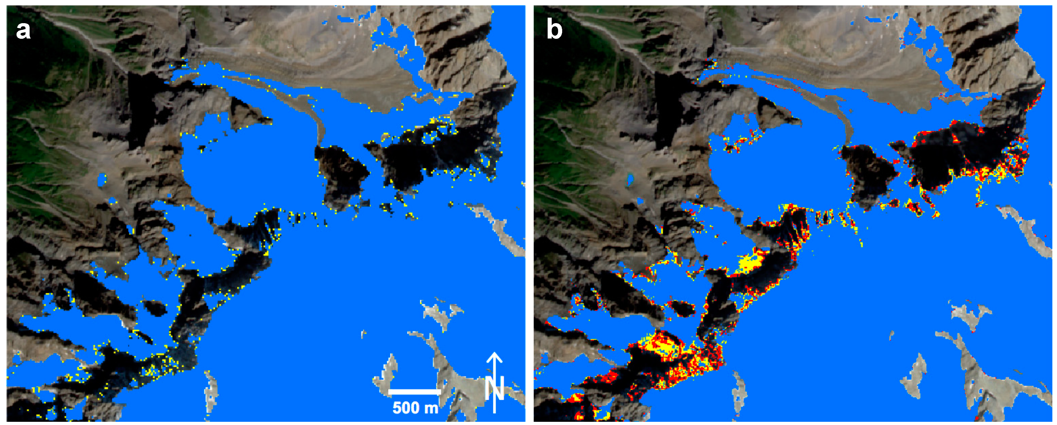
3.4. Mapping Snow and Ice Facies in Test Region 3 (Austria)

To classify snow on glaciers it is required to compensate for atmospheric and topographic effects using a DEM. The required slope and aspect maps were derived from the ASTER GDEM2, which was transformed to the map projection (UTM Zone 32N) of the MSI scene and resampled to 10 m pixel size. The SWIR bands were resampled to 10 m pixel size using nearest neighbor interpolation. We then calculated the top of atmosphere reflectances of all VNIR and SWIR bands of MSI and rescaled them to the value range between 0 and 1. Solar illumination effects were reduced for all bands by applying a topographic correction [32]. They were used as input for computation of four band ratios: (g) the NDSI; (h) the used red/SWIR ratio as in (a); (i) the ratio of the blue (MSI2) and red band (MSI4); and (j) the NIR/SWIR (MSI8/MSI11) ratio as in (c). To be identified as part of the glacier facies, a pixel had to meet all of the following four rules:

(g)

NDSI ≥ 0.20;

(h)

0 ≤ MSI4/MSI11 ≤ 2;

(i)

MSI2/MSI4 ≤ 1.20;

(j)

0 ≤ MSI8/MSI11 ≤ 1.

As glaciers in Austria can only be found above 1800 m [33], the ASTER GDEM2 was used to select only pixels above this altitude. Misclassified pixels, such as water bodies, which are not covered by available water body masks or bright rocks, were manually removed. The derived preliminary glacier facies map is then used in a final step to discriminate snow and bare ice areas on glaciers by applying a threshold on the topographically corrected NIR band MSI8. The manual threshold selection for identifying snow areas on glaciers is based on a step-wise approximation and visual intercomparison of intermediate snow areas with different band composites of the MSI scene following the approach suggested by [19]. Debris-covered glaciers are mapped manually.

4. Results

4.1. Threshold and Band Ratio Tests on MSI in Region 1

Assigning th1 to the threshold for the respective band ratio and th2 to the blue band threshold, we find that the values chosen for th1 have some impact on the mapped extent for snow and ice in direct sunlight (Figure 3), whereas th2 causes little or no change. This is vice versa for ice and snow in shadow, i.e., a change in th1 has little impact but th2 has a strong one (Figure 4a). This points to the well-known requirement to first pick th1 to get all possibly important snow and ice pixels included and then restrict the intermediate results again by removing wrongly mapped bare rock in shadow using th2. The special challenge is to find values for th1 and th2 that achieve a good performance over the entire scene [34]. Depending on the local illumination conditions (e.g., regions with snow in sunlight can considerably brighten nearby regions with ice in shadow), these can vary so that the chosen th1 and th2 pair is always a compromise, even within a single scene.

A related high sensitivity to th1 is also given for mixed pixels as illustrated by the strong variability in mapped extents for regions showing thin snow cover around the nunataks as depicted in Figure 3. Water bodies can be misclassified as glaciers, but this is strongly dependent on their turbidity and thus varies from place to place. We found that MSI8/MSI11 maps fewer water-pixels compared to MSI4/MSI11 and MSI4/MSI12, and is therefore less sensitive on turbid lakes. However, none of the band ratios exclude glacier lakes completely.

The MSI4/MSI11 ratio performs better than the other two ratios with only small differences in mapped glacier extents compared to the MSI8/MSI11 or MSI4/MSI12 ratios (Figure 4b). Hence, the latter is mapping more of the seasonal snow (for the same threshold th1), whereas the former only shows variability at the pixel level, even in regions of shadow. Overall, when applying the band ratios MSI4/MSI11 and MSI8/MSI11 to the S2A images, the results correspond to earlier findings using Landsat band ratios TM3/TM5 and TM4/TM5, respectively [35]. The spatial variability in shadow when using these two ratios with the same th1 and th2 is approximately within a Landsat pixel (30 m) (Figure 4b).

4.2. Glacier Mapping in Test Region 2 with MSI and OLI

When comparing the red/SWIR ratios of S2A (MSI4/MSI11) with the Landsat 8 pan/SWIR ratio (OLI8/OLI6), they appear after some contrast stretching very similar. Both show ice and snow in shadow with higher grey values than the surrounding bare rock. However, it was not possible to clearly separate these with a single threshold using MSI. When all ice and snow in shadow is included in one place, considerable bare rock is wrongly mapped at another place. It was thus required for MSI to use an additional blue band to improve the mapping of ice and snow in shadow [7]. On the other hand, for the OLI8/OLI6 ratio the threshold th1 was sufficient for a precise delineation as Figure 5a demonstrates. Reducing th1 from 1.4 (blue) to 1.38 (blue + yellow pixels) results in some minor changes in regions of shadow. A comparable extent was achieved with MSI (Figure 5b) using a th1 value of 2.7 for the MSI4/MSI11 ratio and an additional th2 value of 95 in the blue band (MSI2). For a slightly higher th2 value of 105 (115) the red (red and yellow) pixels would have been removed and mapping of glaciers in shadow would be inferior to Landsat 8 OLI. As also visible in Figure 4a, the th2 threshold is very helpful in adjusting glacier extents.

A direct comparison of the outlines derived from OLI red, OLI pan and MSI (Figure 6) shows that the latter two are generally contained in the first, as the larger pixel size (30 m) and the inclusion of mixed pixels result in larger glacier extents (for clean ice). However, overall the same regions and spots are mapped. Considering a small (non-systematic) shift between the MSI and OLI images (see Part I for details [18]), outlines from OLI pan (15 m) and MSI (10 m) are more or less coincident (Figure 6) and glacier extents are similar except in regions of topographic shadow.

We have not performed a quantitative comparison to ground-based reference data due to lack of such data during image acquisition. Moreover, obtaining such data is difficult as it requires walking around the entire perimeter of a glacier (e.g., with a hand-held DGPS) and isolated measurements (e.g., at a glaciers terminus) would only reveal well-known geolocation issues [18]. However, we performed a cross-comparison of glacier extents for 155 glaciers, revealing the relative area differences between OLI pan and OLI red, MSI and OLI red, and MSI and OLI pan (Figure 7). On average, MSI-derived outlines for clean ice are 0.7% ± 8.1% smaller than from OLI pan (OLI8/OLI6) and 4.8% ± 10.6% smaller than from OLI 30 m bands (OLI4/OLI6). Comparing only the two OLI band combinations gives 4.2% ± 9.6% smaller glacier areas with OLI pan compared to OLI red. The scatter plot in Figure 7 reveals that glacier areas are systematically smaller with the higher resolution bands from OLI and MSI, and differences increase towards smaller glaciers. For MSI and OLI pan the scatter increases toward smaller glaciers but values are more evenly distributed around zero, indicating that sometimes MSI outlines are smaller, sometimes larger. The latter might also be related to two days of intense snowmelt between the images (MSI was acquired two days before).

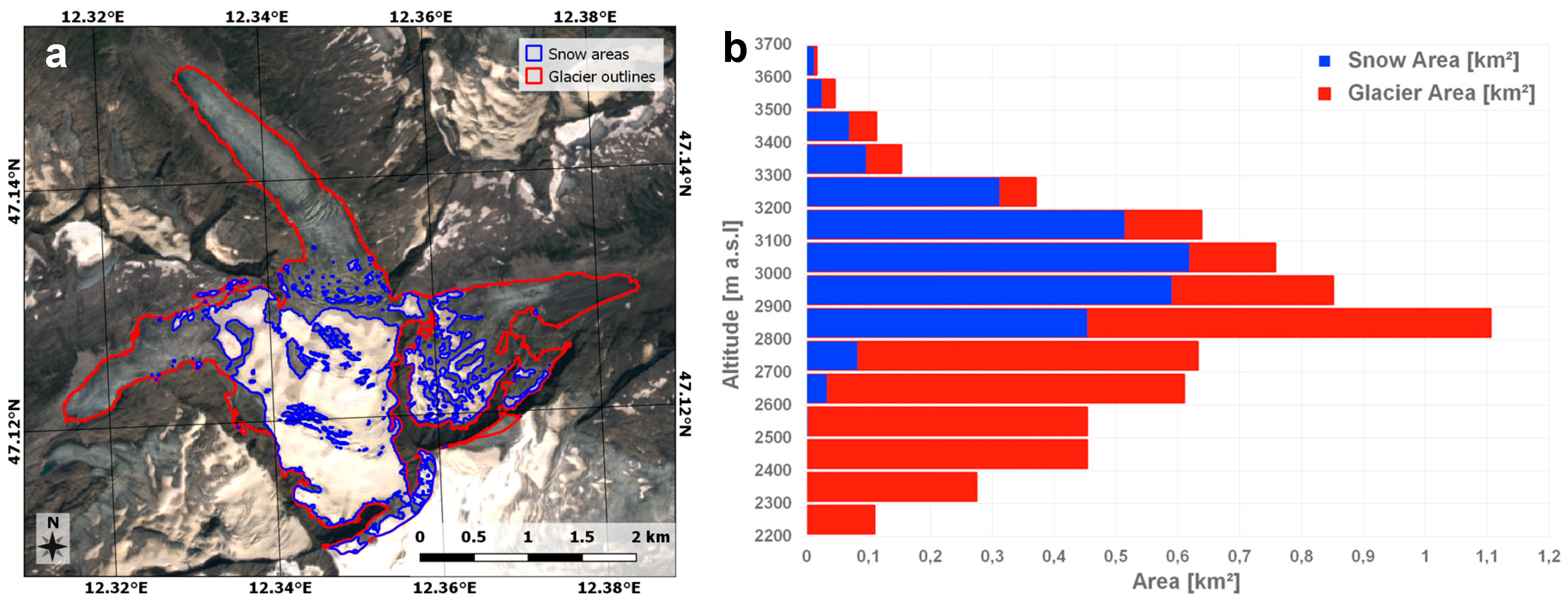
4.3. Snow and Ice Facies

The method described for retrieving glacier facies was applied to a subset of the MSI L1C scene, covering the Hohe Tauern range in the Austrian Alps on 13 August 2015 (Figure 8a). Clear glacier ice and snow areas are automatically mapped, manual corrections are applied in some snow areas in cast shadow, and at debris-covered glacier parts at lower elevations (Figure 8a), and for removing minor misclassifications of bright rocks or small water bodies. The area elevation distribution of the glacier facies indicates that the snow line on the selected glacier region is between 2800 and 2900 m (Figure 8b). The MSI sensor combines a high spatial resolution with a good radiometric performance of visible bands in illuminated snow covered regions, where visible bands of other optical sensors are often saturated.

Whereas the selected area was acquired under nearly clear-sky conditions, areas hidden by cloud cover or cloud shadows have to be masked. Cumulus clouds can be detected and removed by just applying the NDSI, the band ratios and the selected thresholds, but hardly detectable clouds, such as thin clouds over snow covered areas, are more problematic. When they are not detected with the new Cirrus band (available on both MSI and OLI) they have to be masked manually.

5. Discussion

5.1. Combination of Sentinel-2 MSI Band Ratios and Threshold Sensitivity

Applying different Sentinel-2A band combinations in the calculation of band ratios (MSI4/MSI11, MSI8/MSI11 and MSI4/MSI12) gives similar results, especially between the two often used band ratios MSI4/MSI11 and MSI8/MSI11. Results did not improve when changing the SWIR band from MSI11 to MSI12; actually the latter seems to be more sensitive and includes more mixed pixels (thin layer of seasonal snow). The increased spatial and radiometric resolution of S2A gives more possibilities for fine-tuning the thresholds applied on band ratios. However, this step is more sensitive due to the increased variation of pixel values, which benefits glacier mapping, and also creates new challenges. If the satellite image has a thin and/or patchy snow cover, the number of wrongly classified mixed pixels will increase. On the other hand, with the increased temporal resolution of S2A and 2B the interpreter will most likely have a wider selection of scenes to choose from, particularly in cloud and snow covered maritime regions.

The process of manually selecting the best threshold value within one satellite scene requires some effort and investigation time by the interpreter. Various mapping conditions must be taken into account; snow and glacier surface in sun light, in shadowed areas, and potentially in regions with thin snow cover. This is a general problem for all optical sensors, but the increased variation in 12-bit images compared to the former Landsat TM/ETM+ 8-bit images along with the increased spatial resolution, makes glacier mapping more demanding. Application of the threshold th2 on MSI2 is still important for snow and ice detection in regions of cast shadow. Even if an appropriate scene for glacier mapping is found, manual corrections are required for debris covered ice and to exclude seasonal snow attached to glaciers. Lakes with variable turbidity are classified as glaciers, but this to some degree depends on the band ratios and thresholds used. Equivalent to the TM4/TM5 ratio, the MSI8/MSI11 ratio maps less lake area as glaciers than the MSI4/MSI11 (i.e., TM3/5) ratio. The additional application of a normalized difference water index (NDWI) might help detecting these lakes [36], but their manual removal from the final glacier map is still needed.

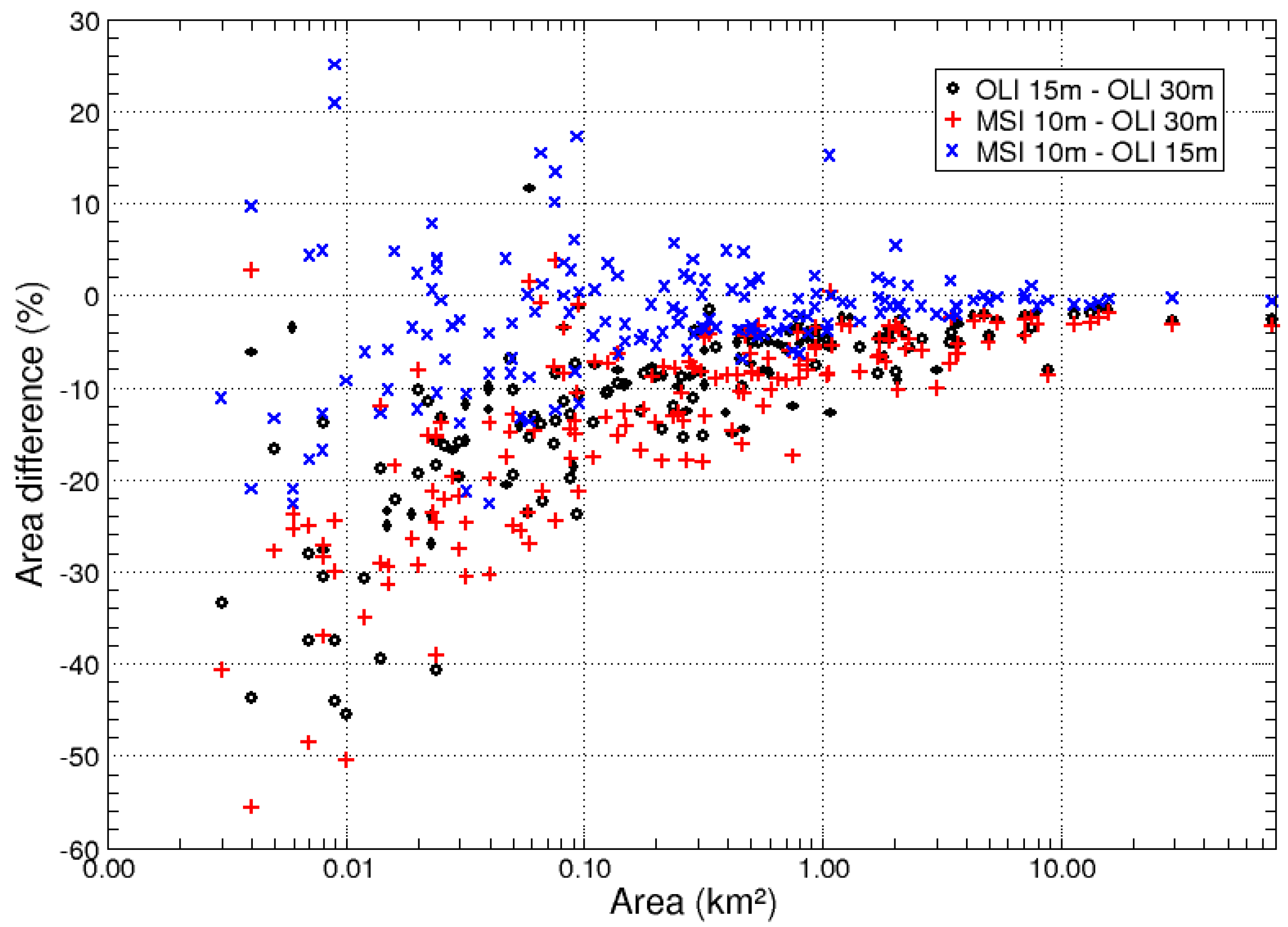
5.2. Glacier Mapping with MSI Compared to OLI

Glacier mapping with the 15 m resolution panchromatic OLI band 8 gives basically the same outlines as with MSI. The OLI band ratio has a reduced workload, as an additional threshold in the blue band was not required for accurate mapping in regions of shadow. A reason that the band ratio method works with the panchromatic band is related to the modified spectral coverage (see Table 2) that now covers the red and the green part of the spectrum. As the respective bands (TM2 and TM3) have been successfully applied in numerous glacier-mapping studies (TM2 with the NDSI), the good results are not surprising. So the question is, if it is worth applying only the OLI8/OLI6 ratio from now on (instead of OLI4/OLI6) considering the smaller glacier size (−4.2% on average) obtained. One can also ask, are the obtained outlines at 15 m (or 10 m for MSI) more precise than with 30 m resolution? This is difficult to answer in general as there are two opposing effects: On the one hand, a former comparison of TM-derived glacier outlines with manually digitized extents indicated that the former are a few percent smaller [37], so getting even smaller extents would be worse. On the other hand, it has been shown [38,39] that the limited spatial resolution of TM does not properly recognize very small glaciers (e.g., <0.1 km²) or they are even undetectable (e.g., in shadow or under debris cover). For a region that is dominated by small glaciers such as the Alps, the higher spatial resolution should give more accurate results [38].

However, there are further important issues requiring consideration: Many glaciers are slightly to fully covered by debris (see Figure 6) and confusion of ice with perennial snowfields is a common obstacle. In both cases the higher spatial resolution, in particular of the MSI sensor, is a great advantage for a more accurate interpretation of the ‘true’ glacier boundary under challenging conditions (see Figure 2) as well as for distinguishing them from snowfields. Moreover, with the 10 m resolution MSI data glacier characteristics such as crevasses became clearly visible and illumination differences due to topographic variability in regions of sunlit snow appear. Both help in the interpretation and correction of outlines. Hence, the outlines derived from MSI (and partly also a pan-sharpened OLI image) will be more accurate whenever manual editing is applied. However, the higher resolution comes at the expense of a higher workload required for editing, as thin medial moraines as well as polluted ice along the glacier boundary will no longer be included in mixed pixels but sharply separated. Applying a spatial filter for noise reduction will partly alleviate this problem, but at the expense of less accurate mapping.

With data from the Sentinel-2A commissioning phase, we used two thresholds th1 and th2 for glacier mapping, whereas OLI only required th1. The former might change when the operational MSI products become available, but the general applicability of the band ratio method previously applied to Terra ASTER or Landsat sensors (TM, ETM+) will likely not change. A recalibration will have little impact on the results related to pixel size. As discussed in Part I of this paper [18], the higher spatial resolution of MSI has advantages for other products. For example, flow velocities can be obtained for small glaciers or the time interval between two images can be reduced.

5.3. Classification of Ice and Snow Facies

The threshold-based method for retrieving glacier facies developed originally for Landsat was adapted for Sentinel-2A, and tested for glaciers in the region Hohe Tauern, Austria. Snow and bare ice were automatically mapped based on topographically corrected top of atmosphere reflectances (TOAR). Correction of topographic illumination effects requires a high quality DEM (pixel spacing in the order of the resolution of the sensor) and accurate geolocation. Unfortunately, the geometric quality of currently available Level 1C data is restricted by the coarse resolution of the DEM used for the orthorectification (PlanetDEM with 90 m spacing). Using a different DEM for the image processing than for the orthorectification can introduce geolocation problems in high and steep terrain. We tested this by using a national airborne laser scanning DEM with 10 m cell size for the topographic correction of the MSI scene and found a significant systematic shift of illuminated and cast shadowed areas. After applying the topographic correction using the ASTER GDEM2, the extended radiometric range of the MSI sensor enabled a clear classification of snow on glaciers that is not restricted by saturation. Due to the high spatial resolution of the VNIR bands even small snow patches remaining near crevasses or in lower parts of the glacier are detected. However, manual correction was required for debris cover and some regions in cast shadow.

5.4. Consequences of the High Temporal Resolution

An increased availability of appropriate images can be expected with Sentinel-2A and 2B. As frequent cloud cover and adverse snow conditions are a major obstacle for creating precise glacier inventories in many regions of the world [9,10,11,12,13,31,35], the shorter repetition interval (5 days at the equator and less towards the poles) might allow obtaining for some regions in the world their first useful dataset. In such a case the potentially higher workload for editing will not play a major role. Moreover, many new glaciological applications will emerge from the frequent data availability (e.g., measuring annual length changes of glaciers) and denser time series (e.g., mass balance estimations from snow lines). For glaciological and hydrological applications requiring high spatial resolution and dense temporal coverage, this will certainly be the start of a new era. A new challenge will be the processing of all the images and their transformation into useful products. This might inspire new frameworks for automated data processing and product retrieval [34,40].

6. Conclusions

Our study has shown that both Sentinel-2A and Landsat 8 can be used to continue automated glacier mapping with the band ratio method using raw digital numbers (i.e., calibrated reflectances). Differences among the methods and the two sensors are most obvious for ice in shadow, where the threshold is most sensitive (i.e., results in the largest changes of the mapped area for an incremental change of the threshold). The ratio of choice (e.g., red/SWIR or NIR/SWIR) providing the best results depends on the image conditions (haze and scattering) and the surrounding environment that should not be mapped (vegetation and lakes) and we recommend testing which combination works best.

Owing to the changed spectral range of the 15 m panchromatic band of the OLI sensor (now covering only green and red), a ratio image OLI pan/SWIR can also be used, allowing the mapping of glaciers at 15 m spatial resolution. We notice only small differences in glacier extents from OLI pan/SWIR compared to MSI red/SWIR (<1%), but about 5% larger extents with OLI red/SWIR using 30 m bands. The latter is related to the inclusion of mixed pixels, in particular along the glacier perimeter. The effort required for manual correction of excluded dirty ice along the glacier boundary will thus be larger for outlines derived from MSI and 15 m OLI pan/SWIR. However, the higher spatial resolution allows a more precise digitizing, resulting in a higher quality product. Although we have not explicitly tested it here, we argue that the higher workload for glacier mapping is worth the effort. We used S2A data from the ramp-up and commissioning phase to obtain the above results. Details might change once datasets with the final calibration are released.

Mapping of snow on glaciers with S2A using topographically corrected TOAR also provided promising results, in particular regarding the extended dynamic range of individual bands (avoiding saturation) and the higher spatial resolution (revealing fine spatial details). The latter is also important to identify snow patches off glaciers and exclude them from the outline. As the mapping of snow on glaciers requires accurate correction of illumination differences caused by topography, the DEM currently used for orthorectification of S2A is not sufficient in spatial resolution (90 m) and quality. We thus recommend using a more appropriate DEM and provide it to the community. Otherwise, secondary products like a shadow mask or drainage divides for creating a glacier inventory will not match the position of the glacier outlines, thus requiring a high workload for manual editing and hindering the foreseen automated applications. In this regard, we note that the current careful manual selection of satellite scenes acquired at the end of ablation season with good mapping conditions is a time consuming process that requires development of new quantitative and highly automated methods to exploit the large amount of data in the future from the combined S2A and S2B satellites. Free availability of all data (satellite and DEM) and automated processing chains are key to derive the respective products and provide them to the interested community on a regular basis.

References

1. Wulder, M.A.; Masek, J.G.; Cohen, W.B.; Loveland, T.R.; Woodcock, C.E. Opening the archive: How free data has enabled the science and monitoring promise of Landsat. Remote Sens. Environ. 2012, 122, 2–10. [Google Scholar] [CrossRef]
2. Vaughan, D.G.; Comiso, J.C.; Allison, I.; Carrasco, J.; Kaser, G.; Kwok, R.; Mote, P.; Murray, T.; Paul, F.; Ren, J.; et al. Observations: Cryosphere. In Climate Change 2013: The Physical Science Basis; Contribution of Working Group I to the Fifth Assessment Report of the IPCC; Cambridge University Press: Cambridge, UK, 2013; pp. 317–382. [Google Scholar]
3. Pfeffer, W.T.; Arendt, A.A.; Bliss, A.; Bolch, T.; Cogley, J.G.; Gardner, A.S.; Hagen, J.O.; Hock, R.; Kaser, G.; Kienholz, C.; et al. The Randolph glacier inventory: A globally complete inventory of glaciers. J. Glaciol. 2014, 60, 537–552. [Google Scholar] [CrossRef] [Green Version]
4. Dozier, J. Spectral signature of alpine snow cover from Landsat 5 TM. Remote Sens. Environ. 1989, 28, 9–22. [Google Scholar] [CrossRef]
5. Paul, F.; Kääb, A.; Maisch, M.; Kellenberger, T.; Haeberli, W. The new remote-sensing-derived Swiss glacier inventory: I. Methods. Ann. Glaciol. 2002, 34, 355–361. [Google Scholar] [CrossRef] [Green Version]
6. Albert, T.H. Evaluation of remote sensing techniques for ice-area classification applied to the tropical Quelccaya Ice Cap, Peru. Polar Geogr. 2002, 26, 210–226. [Google Scholar] [CrossRef]
7. Paul, F.; Kääb, A. Perspectives on the production of a glacier inventory from multispectral satellite data in Arctic Canada: Cumberland Peninsula, Baffin Island. Ann. Glaciol. 2005, 42, 59–66. [Google Scholar] [CrossRef]
8. Paul, F.; Bolch, T.; Kääb, A.; Nagler, T.; Nuth, C.; Scharrer, K.; Shepherd, A.; Strozzi, T.; Ticconi, F.; Bhambri, R.; et al. The glaciers climate change initiative: Methods for creating glacier area, elevation change and velocity products. Remote Sens. Environ. 2015, 162, 408–426. [Google Scholar] [CrossRef]
9. Bolch, T.; Menounos, B.; Wheate, R. Landsat-based glacier inventory of western Canada, 1985–2005. Remote Sens. Environ. 2010, 114, 127–137. [Google Scholar] [CrossRef]
10. Frey, H.; Paul, F.; Strozzi, T. Compilation of a glacier inventory for the western Himalayas from satellite data: Methods, challenges and results. Remote Sens. Environ. 2012, 124, 832–843. [Google Scholar] [CrossRef] [Green Version]
11. Rastner, P.; Bolch, T.; Mölg, N.; Machguth, H.; LeBris, R.; Paul, F. The first complete inventory of the local glaciers and ice caps on Greenland. Cryosphere 2012, 6, 1483–1495. [Google Scholar] [CrossRef] [Green Version]
12. Paul, F.; Mölg, N. Hasty retreat of glaciers in northern Patagonia from 1985 to 2011. J. Glaciol. 2014, 60, 1033–1043. [Google Scholar] [CrossRef]
13. Guo, W.; Liu, S.; Xu, J.; Wu, L.; Shangguan, D.; Yao, X.; Wei, J.; Bao, W.; Yu, P.; Liu, Q.; et al. The second Chinese glacier inventory: Data, methods and results. J. Glaciol. 2015, 61, 357–372. [Google Scholar] [CrossRef]
14. Paul, F.; Huggel, C.; Kääb, A. Combining satellite multispectral image data and a digital elevation model for mapping debris-covered glaciers. Remote Sens. Environ. 2004, 89, 510–518. [Google Scholar] [CrossRef]
15. Shukla, A.; Arora, M.; Gupta, R. Synergistic approach for mapping debris-covered glaciers using optical-thermal remote sensing data with inputs from geomorphometric parameters. Remote Sens. Environ. 2010, 114, 1378–1387. [Google Scholar] [CrossRef]
16. Racoviteanu, A.; Williams, M.W. Decision tree and texture analysis for mapping debris-covered glaciers in the Kangchenjunga area, Eastern Himalaya. Remote Sens. 2012, 4, 3078–3109. [Google Scholar] [CrossRef]
17. Robson, B.A.; Nuth, C.; Dahl, S.O.; Hölbling, D.; Strozzi, T.; Nielsen, P.R. Automated classification of debris-covered glaciers combining optical, SAR and topographic data in an object-based environment. Remote Sens. Environ. 2015, 170, 372–387. [Google Scholar] [CrossRef]
18. Kääb, A.; Winsvold, S.H.; Altena, B.; Nuth, C.; Nagler, T.; Wuite, J. Glacier Remote Sensing using Sentinel-2. Part I: Radiometric and geometric performance, application to ice velocity. Remote Sens. 2016. [Google Scholar] [CrossRef]
19. Bippus, G. Characteristics of Summer Snow Areas on Glaciers Observed by Means of Landsat Data. Ph.D. Thesis, University of Innsbruck, Innsbruck, Austria, 2011. [Google Scholar]
20. Rabatel, A.; Dedieu, J.-P.; Thibert, E.; Letréguilly, A.; Vincent, C. Twenty-five years (1981–2005) of equilibrium-line altitude and mass balance reconstruction on Glacier Blanc in the French Alps using remote sensing methods and meteorological data. J. Glaciol. 2008, 54, 307–314. [Google Scholar] [CrossRef]
21. Barandun, M.; Huss, M.; Sold, L.; Farinotti, D.; Azisov, E.; Salzmann, N.; Usubaliev, R.; Merkushkin, A.; Hoelzle, M. Re-analysis of seasonal mass balance at Abramov Glacier 1968–2014. J. Glaciol. 2015, 61, 1103–1117. [Google Scholar] [CrossRef]
22. Immerzeel, W.W.; Droogers, P.; de Jong, S.M.; Bierkens, M.F.P. Large-scale monitoring of snow cover and runoff simulation in Himalayan river basins using remote sensing. Remote Sens. Environ. 2009, 113, 40–49. [Google Scholar] [CrossRef]
23. Frei, C.; Schär, C. A precipitation climatology of the Alps from high-resolution rain-gauge observations. Int. J. Clim. 1998, 18, 873–900. [Google Scholar] [CrossRef]
24. Böhner, J. General climatic controls and topoclimatic variations in Central and High Asia. Boreas 2006, 35, 279–295. [Google Scholar] [CrossRef]
25. ESA. Sentinel-2 Mission Status Report. Available online: https://sentinel.esa.int/documents/247904/1943503/Sentinel-2_Mission_Status_Report_11-Period_24-30_Oct_2015 (accessed on 27 June 2016).
26. Paul, F.; Frey, H.; LeBris, R. A new glacier inventory for the European Alps from Landsat TM scenes of 2003: Challenges and results. Ann. Glaciol. 2011, 52, 144–152. [Google Scholar] [CrossRef] [Green Version]
27. Drusch, M.; Del Bello, U.; Carlier, S.; Colin, O.; Fernandez, V.; Gascon, F.; Hoersch, B.; Isola, C.; Laberinti, P.; Martimort, P.; et al. Sentinel-2: ESA’s optical high-resolution mission for GMES operational services. Remote Sens. Environ. 2012, 120, 25–36. [Google Scholar] [CrossRef]
28. Frequently Asked Questions about the Landsat Missions. Available online: http://landsat.usgs.gov/band_designations_landsat_satellites.php (accessed on 1 July 2016).
29. ASTER Instrument Characteristics. Available online: https://asterweb.jpl.nasa.gov/characteristics.asp (accessed on 1 July 2016).
30. Bayr, K.J.; Hall, D.; Kovalick, W.M. Observations on glaciers in the eastern Austrian Alps using satellite data. Int. J. Remote Sens. 1994, 15, 1733–1742. [Google Scholar] [CrossRef]
31. Winsvold, S.H.; Andreassen, L.M.; Kienholz, C. Glacier area and length changes in Norway from repeat inventories. Cryosphere 2014, 8, 1885–1903. [Google Scholar] [CrossRef]
32. Ekstrand, S. Landsat TM-based forest damage assessment: Correction for topographic effects. Photogramm. Eng. Remote Sens. 1996, 62, 151–161. [Google Scholar]
33. Lambrecht, A.; Kuhn, M. Glacier changes in the Austrian Alps during the last three decades, derived from the new Austrian glacier inventory. Ann. Glaciol. 2007, 46, 177–184. [Google Scholar] [CrossRef]
34. Winsvold, S.H.; Kääb, A.; Nuth, C. Regional glacier mapping using optical satellite data time series. IEEE J. Sel. Top. Appl. Earth Obs. Remote Sens. 2016. [Google Scholar] [CrossRef]
35. Andreassen, L.M.; Paul, F.; Kääb, A.; Hausberg, J.E. Landsat-derived glacier inventory for Jotunheimen, Norway, and deduced glacier changes since the 1930s. Cryosphere 2008, 2, 131–145. [Google Scholar] [CrossRef] [Green Version]
36. Huggel, C.; Kääb, A.; Haeberli, W.; Teysseire, P.; Paul, F. Remote sensing based assessment of hazards from glacier lake outbursts: A case study in the Swiss Alps. Can. Geotech. J. 2002, 39, 316–330. [Google Scholar] [CrossRef]
37. Paul, F.; Barrand, N.E.; Baumann, S.; Berthier, E.; Bolch, T.; Casey, K.; Frey, H.; Joshi, S.P.; Konovalov, V.; Le Bris, R.; et al. On the accuracy of glacier outlines derived from remote-sensing data. Ann. Glaciol. 2013, 54, 171–182. [Google Scholar] [CrossRef] [Green Version]
38. Fischer, M.; Huss, M.; Barboux, C.; Hoelzle, M. The new Swiss Glacier Inventory SGI2010: Relevance of using high-resolution source data in areas dominated by very small glaciers. Arct. Antarct. Alp. Res. 2014, 46, 933–945. [Google Scholar] [CrossRef]
39. Gardent, M.; Rabatel, A.; Dedieu, J.P.; Deline, P. Multitemporal glacier inventory of the French Alps from the late 1960s to the late 2000s. Glob. Planet. Chang. 2014, 120, 24–37. [Google Scholar] [CrossRef]
40. Selkowitz, D.J.; Forster, R.R. An automated approach for mapping persistent ice and snow cover over high latitude regions. Remote Sens. 2016, 8. [Google Scholar] [CrossRef]
Figure 1. (a) Test region 1 in the Kunlun Mountains in northern Tibet using a S2A image from 18 November 2015 (FCC with bands 11, 8 and 4 as RGB). Glaciers are divided into entities based on the RGI (yellow); the four largest glaciers are named; (b) Landsat 8 OLI image of test region 2 in the western Swiss Alps acquired on 31 August 2015 (in natural colors). The lower inset shows the full swath and the individual tiles (width: 100 km) of the corresponding MSI scene acquired on 29 August 2015, with the red square marking the tile that is shown in the upper inset on top of the Landsat 8 image. The yellow square in this inset denotes the location of the test regions shown in Figures 2, 5 and 6.
Remotesensing 08 00575 g001
Figure 2. Direct comparison of the spatial resolution of 30 m OLI bands (a); and 10 m MSI bands (b). The larger debris-covered glacier to the left is Breithornglacier; image width is 2.8 km.
Remotesensing 08 00575 g002
Figure 3. A variation of threshold values for MSI4/MSI11 (th1) impacts on the mapped extent of snow and ice in sunlight (th2 is always 1100). Pink indicates the smallest and blue the largest extent of snow and ice. The thick yellow line is from the RGI v.5.0 and indicates glacier extents. Background image: FCC with MSI bands 11, 8 and 4 as RGB. Coordinate grid: UTM zone 45N.
Remotesensing 08 00575 g003
Figure 4. (a) Three different threshold values th2 applied to MSI2 do not change glacier extent in sunlight, but result in strong variations in cast shadow; and (b) three different band ratios (all using th2 = 1100) show minor variations in sunlight and shadow. Coordinate grid: UTM zone 45N.
Remotesensing 08 00575 g004
Figure 5. Threshold sensitivity of OLI (a) and MSI (b). (a) A threshold change from 1.4 to 1.38 removes the yellow pixels; (b) A threshold of 2.7 is used for th1 and 95 for th2 (all colors). Changing them to 2.8 and 105 removes the red pixels, changing th2 to 115 also removes the yellow pixels, i.e., much of the ice in shadow would be missed. Image width is 4.9 km.
Remotesensing 08 00575 g005
Figure 6. Overlay of glacier outlines from MSI4/MSI11 (red), OLI8/OLI6 (yellow) and OLI4/OLI6 (green). Ice in shadow is well mapped, but debris-covered ice is missed. Image width is 4.1 km.
Remotesensing 08 00575 g006
Figure 7. Relative area differences vs. glacier area for 155 selected glaciers and the three ratios shown in Figure 8: OLI 15 m = OLI8/OLI6, OLI 30 m = OLI4/OLI6, and MSI 10 m = MSI4/MSI11.
Remotesensing 08 00575 g007
Figure 8. (a) True-color composite of the Sentinel-2A scene from 13 August 2015 showing a subset of the Hohe Tauern range region (the peak of the Großvenediger is in the lower center) with glacier outlines (red) and the classified snow-covered regions (blue). Image width is about 6 km; (b) Area-elevation distribution of the snow and glacier cover for the region shown in (a).
Remotesensing 08 00575 g008