1. Introduction
Spectral analysis is a powerful technique that involves the analysis of material composition by detecting naturally reflected and emitted electromagnetic waves from various substances [
1]. The advancement of remote sensing technology has rendered the examination of spectral patterns and the generation of cartographic representations delineating distinct materials across extensive terrestrial expanses feasible. Spectral mapping through remote sensing imagery has emerged as a well-established method supporting spatial research endeavors, encompassing diverse fields such as geology [
2,
3,
4,
5], biology [
6,
7,
8], and urban planning [
9,
10,
11]. Remote sensing technology and data play integral roles in geological studies, facilitating the exploration of mineral deposits [
12,
13,
14], petroleum resources [
15,
16], and geothermal energy [
17,
18,
19,
20,
21].
Recently, numerous studies in remote sensing have demonstrated the effectiveness of mineral mapping from satellite images [
22,
23,
24]. Spectral analysis of remote sensing supports geological exploration over a large area. Landsat-8 and Sentinel-2 have been widely adopted among the recent multispectral satellites, along with older satellites like ASTER, which provide open-source data for various purposes, including mineral mapping [
25,
26,
27,
28,
29]. These satellites are equipped with spectral sensors that collect information on specific spectral bands from continuous material spectra. Multiple studies on mineral mapping use spectral analysis to support mineral exploration. For instance, a study utilized Landsat Thematic Mapper (TM) data to map kaolinite and alunite alteration zones [
30,
31]. By analyzing the reflectance spectra and employing a minimum noise fraction, matched filter, and spectral unmixing algorithms, they identified and delineated hydrothermal alteration zones within the study area. In another study, researchers used multispectral satellite imagery (PlanetScope, Landsat8-OLI, and Sentinel2-MSI) to map topsoil properties (clay, sand, organic matter and iron contents, and soil color). By employing a cubist algorithm, they identified and mapped the distribution of topsoil properties, aiding in resource exploration and planning [
32].
Furthermore, advancements in satellite technology have significantly improved mineral mapping capabilities. Mineral traces on the ground are distinctive signs of ore beneath the surface. Another study mapped iron oxides, hydroxides, and hydrothermal alteration with more precise identification and characterization of minerals based on the Crosta algorithm [
33]. In another study, the researcher employed multispectral satellite imagery (ASTER) to map key hydrothermal minerals, revealing three successive zones of alterations, i.e., argillic, phyllic, and propylitic [
34]. This information contributed to a better understanding of the mineral resources in arid regions.
Various algorithms are adopted in mineral mapping using remote sensing [
35,
36,
37,
38]. Among the most widely utilized algorithms are target detection algorithms that analyze a target mineral spectrum through a restricted set of bands to discern the distribution of various minerals. To provide a widespread application of these algorithms, the remote sensing software ENVI 5.7 adopts eight different algorithms [
39], namely, Adaptive Coherence Estimator (ACE) [
40,
41], Constrained Energy Minimization (CEM) [
42,
43,
44], Matched Filtering (MF) [
45,
46], Mixture-Tuned Matched Filtering (MTMF) [
47,
48], Orthogonal Subspace Projection (OSP) [
49,
50,
51], Spectral Angle Mapper (SAM) [
52], Target-Constrained Interference-Minimized Filter (TCIMF) [
51,
53,
54], and Mixture-Tuned Target-Constrained Interference-Minimized Filter (MTTCIMF) [
54,
55].
Some of the research, as mentioned above, has primarily focused on individual algorithm results or examined a single mineral using one of these specific algorithms. The critical question of which algorithm effectively identifies different mineral species still needs to be solved, necessitating extensive research. Additionally, a method that fuses the results of different algorithms has yet to be developed, and no studies have been conducted on how well this fusion will yield results. Consequently, developing an improved algorithm or a combination of algorithms for mineral mapping becomes important. Despite some researchers dedicating efforts to evaluating various spectral mapping algorithms, particularly the eight algorithms featured in ENVI software, most of these studies have not been devoted exclusively to mineral spectral mapping [
55,
56,
57,
58,
59,
60,
61]. Furthermore, some researchers did not validate the results of their geological and mineral mapping outcomes using ground-truth information [
12,
35,
36]. As a result, the effectiveness and quality of different algorithms for targeting geological objects need to be more transparent and requires further research.
Mineral mapping for geothermal exploration is not exempt from the issues mentioned above and encounters comparable challenges, as previously mentioned. The reliability issue of the mapping outputs has always been a subject of concern. Therefore, there is an immediate need to enhance the accuracy of remote sensing mapping algorithms since this progress can significantly save exploration costs and time.
This study assessed the effectiveness of different mineral mapping algorithms and their fusion utilizing ground-truth data from a geothermal site. To accomplish this, we obtained pure spectra derived from samples collected from the geothermal field. Furthermore, we developed a novel framework to fuse the chosen algorithms to improve the accuracy of mineral mapping. We compared the results of different combinations with the Receiver Operating Characteristic (ROC) curves and their Area Under the ROC Curve (AUC) values. The progress made in evaluating mapping accuracy has the potential to enhance geothermal exploration procedures greatly with the exploration of minerals. The key to achieving accurate mineral mapping lies in identifying specific combinations of algorithms for each mineral. Ultimately, the execution of these analyses would have been impractical without accumulating a significant amount of ground-truth data, which serves as the unique contribution of our approach. As far as the authors know, no publication has yet incorporated a comprehensive ground-truthing analysis to evaluate the effectiveness of the mineral mapping algorithm on a large scale.
2. Materials and Method
2.1. Coso Geothermal Field and Materials
The Coso Geothermal Field in Inyo County of Eastern California is in the Mojave Desert’s Coso Range from the Sierra Nevada’s east rim. The map of the Coso Geothermal Field is presented in
Figure 1.
Austin and Pringle initially recognized the potential for geothermal energy production in 1970, leading to extensive exploration and development efforts that culminated in the online operation of power generation facilities at Coso during the 1980s [
62]. Moreover, due to its potential for enhanced geothermal systems (EGS) research and applications, the Coso Geothermal Field was selected as one of the research sites for the US Department of Energy’s FORGE (Frontier Observatory for Research in Geothermal Energy) program [
29,
63].
The local rock units were dominated by a large variety of igneous rocks, including mafic rocks (basalt and gabbro), intermediate rocks (andesite and diorite), and felsic rocks (rhyolite and granite). The latest Quaternary volcanic activity created the major rhyolite domes and pyroclastic coverings at Coso [
64]. The alteration minerals that occurred at Coso Geothermal Field included but were not limited to the following minerals: alunite, anhydrite, calcite, chalcedony, chlorite, epidote, goethite, hematite, illite, kaolinite, montmorillonite, opal, rutile, and smectite [
65]. The research focused on those minerals that obtained spectra from the local samples of Coso. These samples collected from the field research for creating pure spectra were used for field and satellite image analysis.
The geological samples extracted from the Coso Geothermal Field served as the fundamental basis for the field data. Through analysis of 97 samples collected from various locations in Coso, the research allowed us to create ground-truth information and a spectral library specific to the Coso Geothermal Field. The collection of geological samples encompassed multiple locations within Coso, including prominent geothermal sites such as Devil’s Kitchen, Nicol Pad, and Wheeler Pad, as depicted in
Figure 2. It illustrates the distribution of 97 samples gathered at the Coso site within the targeted area. As previously mentioned, samples were taken from critical regions except for the restricted Coso Hot Spring location. These samples underwent spectral analysis using an ASD FieldSpec 4 spectroradiometer, a device that records the reflectance spectra of samples across 2151 wavelength channels ranging from 350 to 2500 nm. Conducting spectral collection in controlled environments helps to eliminate unwanted factors like noise or atmospheric effects. Beyond the initial examination of the samples’ physical attributes in the field, laboratory analysis was performed to determine their potential mineral composition. SEM-based automated mineralogy was utilized on chosen samples to study alteration mineralogy, while portable X-ray fluorescence (pXRF) was employed on most samples to gather supplementary data.
In addition to field data, the satellite data were used for target detection analysis. We downloaded ASTER (The Advanced Spaceborne Thermal Emission and Reflection Radiometer) satellite images, including VNIR (visible and near-infrared, 400 to 1000 nm) and SWIR (Short-Wavelength Infrared, 1000 to 2500 nm) information. The acquired ASTER product in this research was Level 1 Precision Terrain Corrected Registered At-Sensor Radiance (AST_L1T) data, which were created from a single resampling of the corresponding ASTER L1A (AST_L1A) product. The AST_L1T contains calibrated at-sensor radiance corresponding with the ASTER Level 1B. Hence, the AST_L1T was geometrically corrected and rotated to a north-up UTM projection [
66].
2.2. Methods
The research introduces a novel framework, as illustrated in
Figure 3, to produce more accurate mineral maps compared to using a single algorithm. The raw satellite data undergo required preprocessing to facilitate subsequent mineral spectral target detection. Meanwhile, the field data from the research area undergo field data analysis to identify mineralogy, establish a spectral library, and obtain ground-truth information for accuracy assessment. Creating a spectral library within this study ensures higher precision in the mineral mapping process. Subsequently, the preprocessed satellite data and spectral library are employed to execute mineral spectral target detection using eight algorithms shown in the dashed rectangle. The target detection results for various minerals and algorithms are then used to generate mineral distribution density accordingly. The density maps and ground-truth information are utilized to assess accuracy, allowing researchers to select better mapping algorithms concerning performance. Subsequently, the preferred mapping algorithms with enhanced accuracy enable the final fusion of mineral maps to produce refined mineral maps for further analysis and utilization. We have applied the accuracy assessment on the final fusion of the mineral map for comparison with individual methods’ accuracy.
2.2.1. Field Data Analysis
Apart from observing the geological occurrence and condition of the samples, various instruments were utilized to analyze them for potential mineralogy. Some researchers used X-ray fluorescence (XRF) analysis based on a portable device [
67,
68,
69] and Scanning Electron Microscopy (SEM) with a mineralogy-analyzing feature [
70,
71,
72] to accurately understand the content and type of the samples.
In conjunction with proposing and developing a distinctive hyperspectral analysis framework, field samples were collected to obtain pure spectra instead of USGS spectra for spectral analysis, thereby offering valuable suggestions regarding the mineralogy in the samples. This process enabled a more accurate and detailed examination of the mineral composition and facilitated the practical application of the proposed hyperspectral analysis methodology.
Figure 4 shows the fundamental approach for analyzing field samples.
In this study, the ASD FieldSpec 4 Hi-RES NG portable spectrometer was used to collect hyperspectral data from samples. The spectra were analyzed using the CSIRO TSG [
73,
74,
75], the THOR Material Identification tool in ENVI software that adopts the SAM algorithm [
52], and the Fully Constrained Linear Spectral Unmixing (FCLSU) algorithm in MATLAB [
76].
In addition to the hyperspectral analysis, this research used the Bruker TRACER 5i Handheld XRF Analyzer to collect enrichment levels of multiple elements as geochemical supporting information for mineralogy. Furthermore, this research analyzed 12 samples by SEM with the TESCAN TIMA system [
77] and Bruker AMICS system [
72]. The SEM analysis provides detailed mineralogy that consolidates the local mineralogy inference of Coso samples.
Based on the mineralogy study, multiple high-purity spectra of geothermal alteration minerals were selected after in-detail analysis from collected samples, including alunite, chalcedony, hematite, kaolinite, and opal. Furthermore, the early research reviewed the samples’ mineralogy with a focus on the presence of the minerals listed above. The spectral data from the Coso local samples can be used in mineral mapping to better identify the regional targets. Furthermore, the ground-truth data that logged either the positive or negative presence of the target geothermal alternation minerals and the sampling coordinates can be considered the ground-truth information for evaluating the accuracy of the mineral maps. After all these field and laboratory analyses, we produced a pure spectral library for further mineral mapping analysis.
2.2.2. Satellite Data Processing and Mineral Spectral Mapping
The initial stage of potential mineral distribution mapping involves preprocessing satellite images. This preparatory step ensures that the satellite data are appropriately processed and ready for further analysis, enabling the accurate detection and mapping of potential mineral occurrences across the study area.
Figure 5 shows the fundamental approach for the fusion of the mineral map analysis using satellite images. This approach to analyzing satellite data was cross-verified with field data and analyses. Additionally, we created a specialized spectral library for the geothermal fields utilized in this study, opting for this instead of the USGS spectral library. The local spectral library was found to yield better outcomes than those achieved with USGS spectra. This contribution further enhances the research into various cases and fields. Given the absence of a fusion approach in earlier studies, the innovation lies in the fusion method and the algorithm we developed. Our proposed framework and algorithm will greatly assist researchers in identifying the most effective method combinations for a wide range of fields and scenarios. This framework has proven highly adaptable and transferable across various studies, showcasing its success. This approach and framework, along with a range of developed algorithms, can be applied to any other type of individual method mineral analysis map. Thus, this study broadly applies to different cases, sites, and algorithms beyond the selected eight.
As the field data analysis steps have been thoroughly covered in the previous section, there is no need to reiterate them in the flowchart.
The ENVI software was utilized to process ASTER satellite data with radiometric calibration. Subsequently, the research applied the QUAC (QUick Atmospheric Correction) method for atmospheric calibration [
78,
79,
80]. The reflectance values of the ASTER data were then normalized to a range between 0 and 1, allowing for effective comparison with spectra obtained from the Coso spectral library. Since the minerals explored in different layers are different, these differences sometimes intersect in a very small area. To avoid losing as many intersecting areas as possible, we resampled the data to 3 × 3 m. Additionally, any human-made objects in the image were masked, eliminating potential interference from non-natural elements during the subsequent target detection analysis. These preprocesses set the fieldwork for further spectral analysis and mineral mapping studies.
The research employed the Target Detection Wizard tool within the ENVI software to ascertain the potential distribution of various minerals to generate a raw target detection dataset. This dataset comprised all target minerals (alunite, chalcedony, hematite, kaolinite, and opal), each possessing high-purity spectra sourced from the Coso Geothermal Field.
The target detection dataset contained the coordinates of each pixel in the satellite image and the evaluation results produced by each selected algorithm for different target minerals. Additionally, the dataset included the corresponding matching values associated with each target mineral, thereby facilitating the identification and analysis of potential mineral occurrences across the study area. All eight mapping algorithms in ENVI were used for target detection, and preliminary mineral maps were produced.
2.2.3. Mineral Mapping Algorithms
The following subsections explain these eight methods in detail.
Adaptive Coherence Estimator (ACE):
The ACE [
81] algorithm was derived from the Generalized Likelihood Ratio (GLR) [
82]. It calculates the pixel and target spectrum ratio and determines whether both spectra are consistent. Since ACE does not require all the end members to be understood in the research area, it is suitable when the background conditions are unclear or variable [
40,
41]. In addition, the ACE’s result does not vary because of the change in the relative scope of the input spectra dataset.
The calculation of the ACE value is:
where
d is the target spectrum,
x is the pixel spectrum, and
Σ is the background covariance matrix [
55].
Constrained Energy Minimization (CEM):
The CEM algorithm also calculates the consistency based on the target spectrum, pixel spectrum, and background correlation or covariance matrix. Like the ACE algorithm, the CEM algorithm does not require all the end members to be understood in the research area. One of the challenges of the CEM algorithm in multispectral analysis is insufficient dimensionality [
43]. The CEM algorithm is also like the OSP algorithm, which was also covered in this paper, but CEM is better at removing unidentified signals and suppressing noise [
44]. The calculation of the CEM value is:
where
d is the target spectrum,
x is the pixel spectrum, and
Σ is the background correlation or covariance matrix [
55].
Matched Filtering (MF):
The MF algorithm has a concept similar to that of the CEM algorithm. The MF algorithm provides a matching level by calculation from the target spectrum, pixel spectrum, background mean vector, and the background covariance matrix. The MF algorithm does not require all the end members to be understood in the area of interest. The shortcoming of the MF algorithm is the handling of spectral unmixing. Furthermore, the MF algorithm is not ideal for discriminating the targets with similar spectral patterns and eventually provides false positive responses [
46]. The calculation of MF value is:
where
d is the target spectrum,
x is the pixel spectrum,
μ is the background mean vector, and
Σ is the background covariance matrix [
55].
Mixture-Tuned Matched Filtering (MTMF):
The MTMF algorithm is based on the MF algorithm. The difference is that the MTMF algorithm adopts a minimum noise fraction (MNF) transformed image as input. The MNF transformation calculates a score that describes the possibility of each pixel being a mixture of the known target and other background materials. With the better ability to identify and reject false positives, the MTMF algorithm was helpful in the detection and discrimination of minor target materials that present similar spectra to background materials [
46].
Orthogonal Subspace Projection (OSP):
The OSP algorithm has a theory that is related to the MF and CEM algorithms. The algorithm reduces the dimensionality and removes the response from non-target materials. The OSP algorithm provides satisfactory results when the target spectra have distinct patterns. However, the analytical results could present lower quality if the target and non-target spectra are similar. To apply the OSP algorithm, at least two spectra are necessary to assign the target and non-target. The variation in the input spectra dataset may lead to different results. The calculation of the OSP value is:
where
d is the target spectrum,
x is the pixel spectrum, and
is the orthogonal subspace projector. The calculation of the orthogonal subspace projector was based on the number of bands (L) and the non-target spectra matrix (U) [
55].
Spectral Angle Mapper (SAM):
The SAM algorithm calculates the similarity between a target and reference spectrum. Both spectra are considered a vector in an n-dimensional space, where n is the number of bands. If the angle between two vectors is 0, the two vectors are the same. Therefore, the smaller SAM value means that the two spectra are similar. The SAM algorithm does not require end members to be understood in the research area. The calculation of the SAM value is:
where
d is the reference spectrum, and
x is the pixel spectrum [
55].
Target-Constrained Interference-Minimized Filter (TCIMF):
The TCIMF algorithm is a modification based initially on the ACE algorithm. While detecting the target material, it also establishes a filter that eliminates the influence of non-target materials. Like the OSP algorithm, this algorithm requires at least two spectra to identify the target and non-target materials for analysis. The variation in the input spectra dataset may lead to different results. The calculation of the TCIMF value is:
where x is the pixel spectrum,
d is the target spectrum,
U is the non-target spectra matrix,
p is the number of target spectra,
q is the amount of non-target spectra, and
R is the background correlation or covariance matrix [
54,
55].
Mixture-Tuned Target-Constrained Interference-Minimized Filter (MTTCIMF):
The MTTCIMF algorithm utilizes the MTMF and TCIMF algorithms. Therefore, it needs MNF transformation for its input as the MTMF. It also requires at least two spectra to identify the target and non-target materials, such as TCIMF. The variation in the input spectra dataset may lead to different results. However, the MTTCIMF algorithm can potentially provide better analysis than the MTMF [
55].
The proceeding of the algorithms OSP, TCIMF, and MTTCIMF requires the understanding of background conditions and the assignment of non-target spectra. Since this research used the five high-purity mineral spectra from the Coso spectral library as the targets, those other than the target spectrum will be identified as non-target spectra. However, it is difficult to identify all of the mineral occurrences of an area, which also brings the challenge of identifying all non-target end members.
With the preliminary target detection data, this study adopted an R Script designed to generate fusion mineral maps as grid data [
22,
83]. After applying each respective method, a new mineral map was generated. These maps are composed of grid pixels, each representing the likelihood of the presence of a designated mineral. Upon the execution of eight distinct algorithms for selected minerals, a total of eight mineral maps were produced. The fusion algorithm utilized quartile methods to identify pixels with the highest probability values by combining the mineral maps. The fusion approach has the advantage of isolating pixels with the highest probability rather than simply consolidating maps from the eight algorithms. The fusion algorithm facilitates the precise allocation of target minerals, the selection of appropriate mapping algorithms, and the establishment of mapping thresholds, thereby enabling the efficient creation of fusion mineral maps across various quartiles. The quality metrics guide the user in determining which combination of methods is best suited for their study field and case. Users can then fuse the chosen algorithms using the same approach, employing the developed algorithm. We used a 0.99 threshold to obtain the highest target mineral probability pixels for further analysis in eight algorithms. The fusion of mineral maps provides a single grid map of preliminary mineral maps of eight algorithms. The research processed the raster data of mineral maps with a Python script that calculates the point density and generates density maps of different minerals and algorithms. The density maps better illustrate the distribution of various minerals based on different mapping algorithms. All visual outputs and basic visual representations are visualized in ArcDesktop 10.4.1 software.
2.3. Quality Metrics
We developed and employed a Python-based density algorithm to analyze the ground-truth point data and the mineral density maps to assess accuracy. The Python script was developed explicitly for density analysis to ascertain the likelihood of specific mineral occurrences in a given area. By scrutinizing the density maps, the script could identify transitions from high to low density, thereby establishing an appropriate threshold for positive or negative occurrences of the target mineral. Additionally, the Python script facilitated a comparative analysis between the mineral density maps and the ground-truth points, constructing a confusion matrix detailing the outcomes of mineral occurrences. The confusion matrix encompassed information on true positive, false positive, true negative, and false negative instances.
Table 1 shows the matrix that enabled the computation of various performance metrics, including the accuracy, precision, recall, F1 score, and ROC curve with AUC, for different mapping algorithms.
Subsequently, through a ranking process based on the accuracy assessment results, the research could discern the mapping algorithms that exhibited superior performance in targeting the desired mineral. Building upon these findings, we selected the more accurate mapping algorithms and combined their results to generate a refined mineral mapping. This fusion approach yielded mineral maps with improved accuracy, enhancing the potential for geothermal resource exploration at the Coso Geothermal Field.
After applying the fusion algorithm to different methods, we compared the quality of the various fusion options with ROC curves. A ROC curve typically presents a graphical representation of two key performance metrics for a classification model. The
x-axis illustrates the false positive rate, representing the number of cases incorrectly identified as positive out of the total negative cases. The
y-axis showcases the true positive rate, also known as recall or sensitivity [
84].
Once all the true/false positives and true/false negatives were identified, the true positive rate and false positive rate were calculated as
3. Implementation of Proposed Framework
After preprocessing the data downloaded from the USGS website and data collected from the field, we employed the Mineral Spectral Target Detection method available in ENVI, indicated in
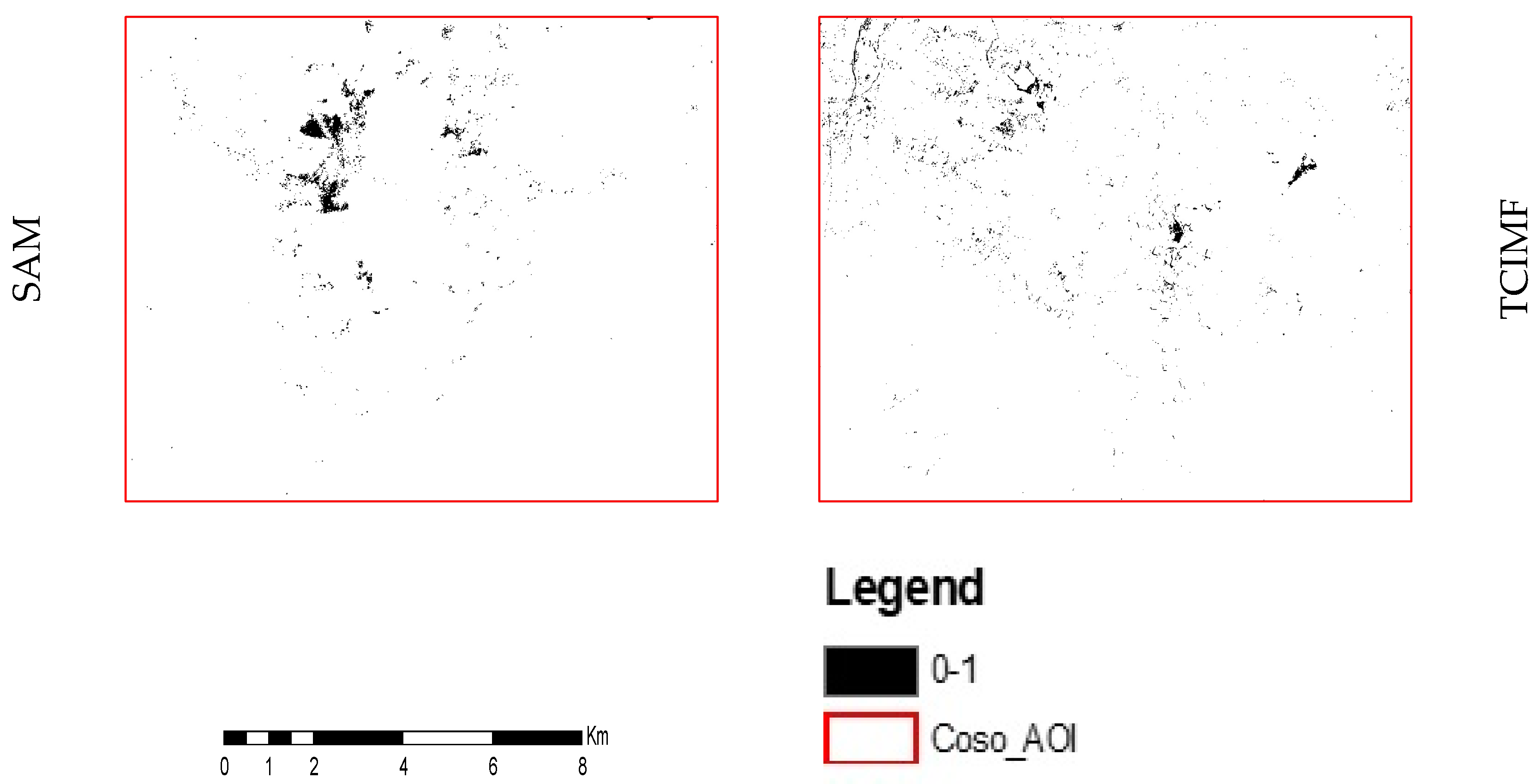
Figure 5 with the spectra we created with the data collected from the field. Instead of visualizing all analysis results in this paper, the opal map results for eight algorithms are visualized in
Figure 6. All other analyses are shared using the link provided in the attachment section at the end.
Since the mineral maps’ results could be too sparse to calculate the accuracy assessment, we created the mineral map’s density, as shown in
Figure 7. It reveals a notable similarity in the distribution patterns among the mapping algorithms CEM, MF, and MTMF. TCIMF, OSP, and MTTCIMF results also show a similar distribution pattern among themselves.. These observations suggest a certain level of agreement or consistency in the results obtained from these algorithmic approaches.
We executed the accuracy assessment, incorporating the preliminary mineral maps and the ground-truth data obtained from the Coso Geothermal Field as input. These maps were transformed into density maps, illustrated for opal minerals with the ACE algorithm in
Figure 8, to facilitate intermediate data visualization during the evaluation process. We aimed to comprehensively evaluate each mapping algorithm’s performance through the accuracy assessment, enabling us to identify and select the most effective algorithms for producing reliable mineral maps. This process is essential for ensuring the accuracy and quality of the final mineral mapping results, thereby facilitating meaningful insights for geothermal resource exploration in the Coso Geothermal Field.
Table 2 presents the accuracy results of different mapping algorithms concerning selected minerals. Through a systematic analysis, the research identified distinct thresholds that effectively segregated the results into two groups: one displaying higher accuracy and the other with lower accuracy. This categorization comprehensively evaluated each algorithm’s performance on individual minerals.
Table 2 compares the accuracy of each method for each mineral to decide which methods should be fused to have the best mineral alteration map.
In
Table 2, the research highlights the mapping algorithms that demonstrated higher accuracy for each mineral. By counting the occurrences of better performance higher than 68% (rightmost column in
Table 2) for each algorithm across all minerals, a decision was made regarding selecting algorithms to be fused in the subsequent stages. This approach allowed the researchers to prioritize and combine the mapping algorithms that exhibited superior performance, thus aiming to create refined and robust mineral maps.
Based on the outcome of the accuracy assessment, it is evident that the algorithms CEM, MF, and MTMF exhibited significantly better accuracy performance than the other algorithms. CEM, MF, and MTMF produced closely matched results statistically and visually among these eight algorithms. On the other hand, SAM demonstrated a moderate level of performance, while ACE, OSP, TCIMF, and MTTCIMF showed poorer performance with results that were also quite similar.
Compared with earlier studies [
57,
59], as shown in
Table 3 below, this study also showed that CEM, MF, and MTMF perform better among the eight algorithms. Meanwhile, TCIMF, OSP, and MTTCIMF have worse performance. This table proves the reliability of the compatibility of these three research results. This earlier research evaluated the individual algorithm’s performance but did not fuse the different combinations of algorithms and their performance, which makes this study unique compared to the previous studies.
Moreover, the ROC curve with AUC values is a good indication for the researchers to compare the individual algorithm results with the different combinations.
The individual algorithms give different AUC values (
Figure 9) ranging from 0.24 to 0.99 for this mineral and this case. As noticed, the accuracy results are varied and inconsistent in other minerals for individual algorithms. Thus, we deduce that particular algorithms do not always produce optimal outcomes for all cases and minerals. For example, ACE is 0.24 for this case, but it may have the best result with the highest AUC value in another case and mineral. Therefore, the red line, the fusion of the eight algorithms for opal in this case, has the highest AUC values and the best ROC curve.
Therefore, based on these findings, we have exclusively selected the CEM, MF, and MTMF algorithms to finalize the refined mineral maps. However, the study finally proves that the fusion of different options in any case is better than using individual methods. Therefore, we fused three, four, five, and eight algorithms and compared them with the ROC curve and AUC values (
Table 4). Finally, we developed and proposed a framework with the R and Python code for fusing selected algorithms by calculating their performance and accuracy.
The research aims to ensure the highest accuracy and reliability in creating fused mineral maps by utilizing these selected algorithms. These maps are expected to be valuable assets in advancing geothermal resource exploration at the Coso Geothermal Field. Moreover, this study aims to prove that the fusion of different algorithms systematically gives better results than using the individual method for mineral mapping.
Figure 10 shows the ROC curve and AUC values for different fusion options, including the results of the fusion of three, four, five, and eight algorithms. It proves which option in total is better than the other options. Even if we indicated that the fusion of mineral maps, in any case, gives better results than using individual algorithms, it would be logical to have better results with the best combination of the algorithms. For this purpose, the ROC curve with the AUC values helps to decide which combination is better. Accordingly, eight-algorithm fusion works better in alunite, hematite, and opal minerals, as indicated by a red color line. AUC values are 1.0, 0.959, and 0.991 for alunite, hematite, and opal minerals.
On the other hand, three- and four-algorithm fusion methods work better in chalcedony and kaolinite. Their AUC values are 0.913 and 0.921, respectively.
Figure 11 shows the fusion of three, four, five, and eight algorithms for all minerals but visualizes only opal. The highest mineral alteration is observed in the eight-algorithm fusion; on the contrary, the lowest mineral alteration of fusion maps is observed in three-algorithm fusion maps, as expected.
4. Results and Discussion
Before evaluating the fusion density maps of opal, we should determine the individual algorithm results shown in
Figure 8. The result of ACE algorithms does not reveal any cluster of minerals at Coso Hot Spring and Devil’s Kitchen. Only one primary cluster is indicated on the northwest of the field. From the ground-truth information, we know that there are opal minerals at Devis’s Kitchen and Coso Hot Spring but not in the northwest.
Figure 11 displays the algorithm fusion map of opal, revealing the identification of two or more prominent opal clusters. Notably, these clusters precisely correspond to Coso Hot Spring and Devil’s Kitchen locations, which are significant regional geothermal landscapes. This alignment reinforces the accuracy and effectiveness of the mapping results, indicating a successful identification of opal occurrences in these key geothermal areas. Similar results and findings have also been revealed in the other minerals.
The opal density map obtained from the fusion of the three algorithms is shown in
Figure 12. Furthermore, the density mapping process detected a disseminated opal pattern northwest of the Coso Geothermal Field. Detecting this disseminated pattern contributes valuable insights into the distribution of opal in the broader vicinity of the geothermal field.
The opal density map obtained from the fusion of the four algorithms is shown in
Figure 13. The analysis result shows that there are clusters in Coso Hot Spring and Devil’s Kitchen. Density at Devil’s Kitchen and Coso Hot Spring is lower than detected by the fusion of the three algorithms. On the contrary, the mineral density in the northwest is higher than that detected by the fusion of the three algorithms.
Figure 14 shows the map for the fusion of five algorithms and density map of opal. The map does not show any significant clusters; however, it does show some small clusters near Coso Hot Spring and Devil’s Kitchen. The outcome of combining five algorithms is comparable to that of combining four algorithms. Adding one or two more algorithms did not yield any improvement in the results.
Furthermore, the mapping process revealed the presence of several major opal clusters at the northeast and middle of the Coso Geothermal Field. As for the fusion of opal, depicted in
Figure 15, it highlights two major opal clusters located precisely at the positions of Coso Hot Spring and Devil’s Kitchen. This finding indicates a concentrated accumulation of opal in these specific regions, potentially making it an area of interest for further mineral investigations and resource assessments.
Ultimately, these fusion mineral maps play a critical role in improving geothermal exploration’s accuracy, efficiency, and effectiveness, offering valuable information for researchers and industries involved in the renewable energy transition. Integrating these maps into geothermal exploration practices can lead to more informed decision-making and pave the way for sustainable and responsible resource utilization in the Coso Geothermal Field and beyond.
Overall, the fusion maps show the capability of the selected mapping algorithms (CEM, MF, and MTMF) to accurately delineate opal occurrences, identify important geothermal features, and recognize additional opal deposits beyond the main geothermal zones. Moreover, the fusion of all eight algorithms results without selection improves the analysis’s quality and provides consistent results. This outcome enhances understanding of the mineral’s distribution and potential implications for exploring geothermal resources in the Coso Geothermal Field and surrounding areas.
5. Conclusions
The primary objective of this research was to facilitate mineral exploration by selecting the best combination of mineral mapping algorithms. In addition, we prove that any combination of fusion of mineral maps is better than the result of the individual algorithm. Specifically, the study focused on assessing the efficacy of eight distinct mapping algorithms for spectral mapping. There is a clear need for more thorough investigations into accurately assessing spectral mapping for minerals and rocks. Specifically, evaluating all eight algorithms simultaneously is essential to ensure a comprehensive evaluation.
To address this research gap, the study introduced an innovative framework designed to evaluate these eight mapping algorithms in the context of spectral mappings. By employing this novel approach, we aimed to provide valuable insights into the performance and reliability of each algorithm, thereby enhancing the understanding of their potential applications in geothermal exploration efforts. The individual algorithm result was evaluated with quality metrics and showed that CEM = MF = MTMF > SAM > ACE = OSP = TCIMF = MTTCIMF. This result is compatible with the previous research. In addition, we evaluate the performance of the different fusion options by looking at the ROC and AUC values, which are very important metrics for assessing these types of image analysis results.
The findings of this study hold significant implications for advancing the adoption of renewable energy sources, as accurate spectral mapping is crucial in identifying and harnessing geothermal resources effectively. The research’s pioneering evaluation framework is expected to contribute to optimizing geothermal exploration strategies and facilitating the transition toward sustainable energy solutions.
With adequately established ground-truth information that contains mineral occurrence information, the framework allows researchers to evaluate mapping results from different algorithms. The framework supports the decision of the best mapping algorithm that fits the specific research area of interest, satellite image, or spectral targets. Therefore, the study reviewed all eight mapping algorithms and identified the best combination for further analysis instead of a single specific mapping algorithm.
Furthermore, the result from the framework is more reliable than traditional visual judgment because it is based on ground-truth information and several quality metrics. Ultimately, the proposed framework empowers researchers to make evidence-based decisions, advance the efficacy and precision of spectral mapping applications, and contribute to the successful transition toward renewable energy sources.
As a result, the fusion of eight algorithms for alunite, opal, and hematite minerals, four algorithms for chalcedony minerals, and three algorithms for kaolinite minerals, concerning their accuracy results derived from the framework, is better than the result of individual methods for the minerals alunite, chalcedony, hematite, kaolinite, and opal. Fusion of mineral maps was generated and compiled based on the improved accuracy and reliability of the selected algorithms. Furthermore, our methodology demonstrated that the fusion of all eight available algorithms does not always produce the most precise outcomes for all the minerals under examination. Therefore, investigating algorithm combinations for precise mineral mapping is of utmost importance. Identifying specific combinations for each mineral is the key to achieving accurate mineral mapping. Ultimately, executing these analyses would have been infeasible without accumulating a substantial amount of ground-truth data, which serves as the distinctive contribution of the presented approach. To the best of the authors‘ knowledge, a publication has yet to include a large-scale ground-truthing analysis for assessing the performance of the mineral mapping algorithm.
The study proves satellite images are worth considering for mineral alteration mapping purposes. The mineral alteration map produced with this approach is highly overlapped with the geothermal zones at Coso. This study’s proposed approach and framework are novel and worth using in other rock and mineral extraction mapping approaches.
In this study, a satellite image with specific characteristics was studied in a geothermal area with unique geological features. Therefore, many factors, such as all the features of the satellite image used, the characteristics of the selected area, and its geological structure, may change the results of such studies. For this reason, the applicability of this study to other fields is also the subject of scientific research and needs to be studied in detail.
Author Contributions
Conceptualization, M.C. and S.D.; methodology, M.C., S.D. and Y.-T.Y.; software, M.C., E.D., S.D. and Y.-T.Y.; validation, M.C., S.D., E.D. and Y.-T.Y.; formal analysis, M.C. and Y.-T.Y.; investigation, M.C., S.D., E.D. and Y.-T.Y.; resources, M.C., S.D., E.D. and Y.-T.Y.; data M.C., and Y.-T.Y.; writing—original draft preparation, M.C. and Y.-T.Y.; writing—review and editing, M.C., S.D. and Y.-T.Y.; visualization, M.C., E.D. and Y.-T.Y.; supervision, M.C. and S.D.; project administration, M.C. and S.D.; funding acquisition, S.D. All authors have read and agreed to the published version of the manuscript.
Funding
This research was funded by the US Department of Energy grant number DE-EE0008760. And The APC was funded by DE-EE0008760.
Data Availability Statement
Acknowledgments
We would like to thanks to NASA, USGS, Navy Geothermal Program Office and CSM for their support. We used high-performance computing (HPC) and other facilities at the Colorado School of Mines. We benefitted from the availability of satellite data from NASA’s ASTER projects and USGS. Additionally, we would like to thank Coso Operating Geothermal LLC in Nevada for their support and valuable feedback.
Conflicts of Interest
There is no conflict of interest.
References
- Kokaly, R.F.; Clark, R.N.; Swayze, G.A.; Livo, K.E.; Hoefen, T.M.; Pearson, N.C.; Wise, R.A.; Benzel, W.M.; Lowers, H.A.; Driscoll, R.L.; et al. USGS Spectral Library Version 7; U.S. Geological Survey: Denver, CO, USA, 2017. [Google Scholar]
- Thomas, M.; Walter, M.R. Application of Hyperspectral Infrared Analysis of Hydrothermal Alteration on Earth and Mars. Astrobiology 2002, 2, 335–351. [Google Scholar] [CrossRef] [PubMed]
- Thompson, A.; Scott, K.; Huntington, J.; Yang, K. Mapping Mineralogy with Reflectance Spectroscopy. In Remote Sensing and Spectral Geology; Society of Economic Geologists: Littleton, CO, USA, 2009; pp. 25–40. [Google Scholar]
- Asadzadeh, S.; de Souza Filho, C.R. A Review on Spectral Processing Methods for Geological Remote Sensing. Int. J. Appl. Earth Obs. Geoinf. 2016, 47, 69–90. [Google Scholar] [CrossRef]
- Said, C.; Youssef, H.; Jamal, A.; Ouallali, A.; Mohamed, E.A.; Larbi, B.; Assia, I.; Zineb, A.; Slimane, S.; Lahcen, O.; et al. Litho-Structural and Hydrothermal Alteration Mapping for Mineral Prospection in the Maider Basin of Morocco Based on Remote Sensing and Field Investigations. Remote Sens. Appl. 2023, 31, 100980. [Google Scholar] [CrossRef]
- Beć, K.B.; Grabska, J.; Huck, C.W. Near-Infrared Spectroscopy in Bio-Applications. Molecules 2020, 25, 2948. [Google Scholar] [CrossRef]
- Sagan, V.; Peterson, K.T.; Maimaitijiang, M.; Sidike, P.; Sloan, J.; Greeling, B.A.; Maalouf, S.; Adams, C. Monitoring Inland Water Quality Using Remote Sensing: Potential and Limitations of Spectral Indices, Bio-Optical Simulations, Machine Learning, and Cloud Computing. Earth Sci. Rev. 2020, 205, 103187. [Google Scholar] [CrossRef]
- Cawse-Nicholson, K.; Townsend, P.A.; Schimel, D.; Assiri, A.M.; Blake, P.L.; Buongiorno, M.F.; Campbell, P.; Carmon, N.; Casey, K.A.; Correa-Pabón, R.E.; et al. NASA’s Surface Biology and Geology Designated Observable: A Perspective on Surface Imaging Algorithms. Remote Sens. Environ. 2021, 257, 112349. [Google Scholar] [CrossRef]
- Herold, M.; Roberts, D.A.; Gardner, M.E.; Dennison, P.E. Spectrometry for Urban Area Remote Sensing–Development and Analysis of a Spectral Library from 350 to 2400 Nm. Remote Sens. Environ. 2004, 91, 304–319. [Google Scholar] [CrossRef]
- Fauvel, M.; Spectral and Spatial Methods for the Classification of Urban Remote Sensing Data Spectral and Spatial Methods for the Classification of Urban Remote Sensing Data. Signal Image Process. 2008. Available online: https://mistis.inrialpes.fr/people/fauvel/Site/Publication_files/plan_these.pdf (accessed on 26 March 2024).
- Shafri, H.Z.M.; Taherzadeh, E.; Mansor, S.; Ashurov, R. Hyperspectral Remote Sensing of Urban Areas: An Overview of Techniques and Applications. Res. J. Appl. Sci. Eng. Technol. 2012, 4, 1557–1565. [Google Scholar]
- Mars, J.C. Mineral and Lithologic Mapping Capability of Worldview 3 Data at Mountain Pass, California, Using True- and False-Color Composite Images, Band Ratios, and Logical Operator Algorithms. Econ. Geol. 2018, 113, 1587–1601. [Google Scholar] [CrossRef]
- Cardoso-Fernandes, J.; Teodoro, A.C.; Lima, A.; Perrotta, M.; Roda-Robles, E. Detecting Lithium (Li) Mineralizations from Space: Current Research and Future Perspectives. Appl. Sci. 2020, 10, 1785. [Google Scholar] [CrossRef]
- Sekandari, M.; Masoumi, I.; Pour, A.B.; Muslim, A.M.; Rahmani, O.; Hashim, M.; Zoheir, B.; Pradhan, B.; Misra, A.; Aminpour, S.M. Application of Landsat-8, Sentinel-2, ASTER and Worldview-3 Spectral Imagery for Exploration of Carbonate-Hosted Pb-Zn Deposits in the Central Iranian Terrane (CIT). Remote Sens. 2020, 12, 1239. [Google Scholar] [CrossRef]
- Avcioğlu, E. Hydrocarbon Microseepage Mapping via Remote Sensing for Gemrik Anticline, Bozova Oil Field, Adıyaman, Turkey; Middle East Technical University: Ankara, Turkey, 2010. [Google Scholar]
- Soydan, H.; Koz, A.; Düzgün, H.Ş. Identification of Hydrocarbon Microseepage Induced Alterations with Spectral Target Detection and Unmixing Algorithms. Int. J. Appl. Earth Obs. Geoinf. 2019, 74, 209–221. [Google Scholar] [CrossRef]
- Calvin, W.M.; Littlefield, E.F.; Kratt, C. Remote Sensing of Geothermal-Related Minerals for Resource Exploration in Nevada. Geothermics 2015, 53, 517–526. [Google Scholar] [CrossRef]
- Kratt, C.; Calvin, W.M.; Coolbaugh, M.F. Mineral Mapping in the Pyramid Lake Basin: Hydrothermal Alteration, Chemical Precipitates and Geothermal Energy Potential. Remote Sens. Environ. 2010, 114, 2297–2304. [Google Scholar] [CrossRef]
- Rodriguez-Gomez, C.; Kereszturi, G.; Reeves, R.; Rae, A.; Pullanagari, R.; Jeyakumar, P.; Procter, J. Lithological Mapping of Waiotapu Geothermal Field (New Zealand) Using Hyperspectral and Thermal Remote Sensing and Ground Exploration Techniques. Geothermics 2021, 96, 102195. [Google Scholar] [CrossRef]
- Savitri, K.P.; Hecker, C.; van der Meer, F.D.; Sidik, R.P. VNIR-SWIR Infrared (Imaging) Spectroscopy for Geothermal Exploration: Current Status and Future Directions. Geothermics 2021, 96, 102178. [Google Scholar] [CrossRef]
- Simpson, M.P.; Rae, A.J. Short-Wave Infrared (SWIR) Reflectance Spectrometric Characterisation of Clays from Geothermal Systems of the Taupō Volcanic Zone, New Zealand. Geothermics 2018, 73, 74–90. [Google Scholar] [CrossRef]
- Moraga, J.; Duzgun, H.S.; Cavur, M.; Soydan, H. The Geothermal Artificial Intelligence for Geothermal Exploration. Renew. Energy 2022, 192, 134–149. [Google Scholar] [CrossRef]
- Gürbüz, E. Multispectral Mapping of Evaporite Minerals Using ASTER Data: A Methodological Comparison from Central Turkey. Remote Sens. Appl. 2019, 15, 100240. [Google Scholar] [CrossRef]
- Lamrani, O.; Aabi, A.; Boushaba, A.; Seghir, M.T.; Adiri, Z.; Samaoui, S. Bentonite Clay Minerals Mapping Using ASTER and Field Mineralogical Data: A Case Study from the Eastern Rif Belt, Morocco. Remote Sens. Appl. 2021, 24, 100640. [Google Scholar] [CrossRef]
- Baldridge, A.M.; Hook, S.J.; Grove, C.I.; Rivera, G. The ASTER Spectral Library Version 2.0. Remote Sens. Environ. 2009, 113, 711–715. [Google Scholar] [CrossRef]
- Drusch, M.; Del Bello, U.; Carlier, S.; Colin, O.; Fernandez, V.; Gascon, F.; Hoersch, B.; Isola, C.; Laberinti, P.; Martimort, P.; et al. Sentinel-2: ESA’s Optical High-Resolution Mission for GMES Operational Services. Remote Sens. Environ. 2012, 120, 25–36. [Google Scholar] [CrossRef]
- Roy, D.P.; Wulder, M.A.; Loveland, T.R.; Woodcock, C.E.; Allen, R.G.; Anderson, M.C.; Helder, D.; Irons, J.R.; Johnson, D.M.; Kennedy, R.; et al. Landsat-8: Science and Product Vision for Terrestrial Global Change Research. Remote Sens. Environ. 2014, 145, 154–172. [Google Scholar] [CrossRef]
- Cavur, M.; Moraga, J.; Sebnem Duzgun, H.; Soydan, H.; Jin, G. Displacement Analysis of Geothermal Field Based on Psinsar and Som Clustering Algorithms: A Case Study of Brady Field, Nevada—USA. Remote Sens. 2021, 13, 349. [Google Scholar] [CrossRef]
- Sabin, A.; Blake, K.; Lazaro, M.; Meade, D.; Blankenship, D.; Kennedy, M.; Mcculloch, J.; Deoreo, S.; Hickman, S.; Glen, J.; et al. Geologic Setting of the West Flank, A Forge Site Adjacent to the Coso Geothermal Field. In Proceedings of the 41st Workshop on Geothermal Reservoir Engineering, Stanford, CA, USA, 22–24 February 2016. [Google Scholar]
- Adiri, Z.; Lhissou, R.; El Harti, A.; Jellouli, A.; Chakouri, M. Recent Advances in the Use of Public Domain Satellite Imagery for Mineral Exploration: A Review of Landsat-8 and Sentinel-2 Applications. Ore Geol. Rev. 2020, 117, 103332. [Google Scholar] [CrossRef]
- Ferrier, G.; Ganas, A.; Pope, R. Prospectivity Mapping for High Sulfidation Epithermal Porphyry Deposits Using an Integrated Compositional and Topographic Remote Sensing Dataset. Ore Geol. Rev. 2019, 107, 353–363. [Google Scholar] [CrossRef]
- Silvero, N.E.Q.; Demattê, J.A.M.; de Souza Vieira, J.; de Oliveira Mello, F.A.; Amorim, M.T.A.; Poppiel, R.R.; de Sousa Mendes, W.; Bonfatti, B.R. Soil Property Maps with Satellite Images at Multiple Scales and Its Impact on Management and Classification. Geoderma 2021, 397, 115089. [Google Scholar] [CrossRef]
- Domra Kana, J.; Djongyang, N.; Raïdandi, D.; Njandjock Nouck, P.; Dadjé, A. A Review of Geophysical Methods for Geothermal Exploration. Renew. Sustain. Energy Rev. 2015, 44, 87–95. [Google Scholar] [CrossRef]
- Abdelkareem, M.I. Using of Remote Sensing and Aeromagnetic Data for Predicting Potential Areas of Hydrothermal Mineral Deposits in the Central Eastern Desert of Egypt. Remote Sens. 2018, 7, 1–13. [Google Scholar] [CrossRef]
- Abubakar, A.J.; Hashim, M.; Pour, A.B. Using ASTER Satellite Data for Mapping Hydrothermal Alteration as a Tool in Geothermal Exploration with GPS Field Validation. Adv. Sci. Lett. 2018, 24, 4489–4495. [Google Scholar] [CrossRef]
- Park, H.; Choi, J. Mineral Detection Using Sharpened Vnir and Swir Bands of Worldview-3 Satellite Imagery. Sustainability 2021, 13, 5518. [Google Scholar] [CrossRef]
- Flores, H.; Lorenz, S.; Jackisch, R.; Tusa, L.; Cecilia Contreras, I.; Zimmermann, R.; Gloaguen, R. UAS-Based Hyperspectral Environmental Monitoring of Acid Mine Drainage Affected Waters. Minerals 2021, 11, 182. [Google Scholar] [CrossRef]
- Abedini, M.; Ziaii, M.; Timkin, T.; Pour, A.B. Machine Learning (ML)-Based Copper Mineralization Prospectivity Mapping (MPM) Using Mining Geochemistry Method and Remote Sensing Satellite Data. Remote Sens. 2023, 15, 3708. [Google Scholar] [CrossRef]
- Wolfe, J.D.; Black, S.R. Hyperspectral Analytics in ENVI; September 19, 2018 Edition. Available online: https://www.nv5geospatialsoftware.com/Portals/0/pdfs/Confirmation/L3HG_Hyperspectral_Whitepaper.pdf (accessed on 26 March 2024).
- Kraut, S.; Scharf, L.L.; Butler, R.W. The Adaptive Coherence Estimator: A Uniformly Most-Powerful-Invariant Adaptive Detection Statistic. IEEE Trans. Signal Process. 2005, 53, 427–438. [Google Scholar] [CrossRef]
- Manolakis, D.; Marden, D.; Shaw, G.A. Hyperspectral Image Processing for Automatic Target Detection Applications. Linc. Lab. J. 2003, 14, 79–116. [Google Scholar]
- Harsanyi, J.C.; Chang, C.-I. Detection and Classification of Subpixel Spectral Signatures in Hyperspectral Image Sequences; University of Maryland: Baltimore County, MD, USA, 1993. [Google Scholar]
- Chang, C.-I.; Liu, J.-M.; Chieu, B.-C.; Ren, H.; Wang, C.-M.; Lo, C.-S.; Chung, P.-C.; Yang, C.-W.; Ma, D.-J. Generalized Constrained Energy Minimization Approach to Subpixel Target Detection for Multispectral Imagery. Opt. Eng. 2000, 39, 1275. [Google Scholar] [CrossRef]
- Du, Q.; Ren, H.; Chang, C.I. A Comparative Study for Orthogonal Subspace Projection and Constrained Energy Minimization. IEEE Trans. Geosci. Remote Sens. 2003, 41, 1525–1529. [Google Scholar] [CrossRef]
- Turin, G. An Introduction to Matched Filters. IEEE Trans. Inf. Theory 1960, 6, 311–329. [Google Scholar] [CrossRef]
- Boardman, J.W.; Kruse, F.A. Analysis of Imaging Spectrometer Data Using N -Dimensional Geometry and a Mixture-Tuned Matched Filtering Approach. IEEE Trans. Geosci. Remote Sens. 2011, 49, 4138–4152. [Google Scholar] [CrossRef]
- Boardman, J.W. Leveraging the High Dimensionality of AVIRIS Data for Improved Sub-Pixel Target Unmixing and Rejection of False Positives: Mixture Tuned Matched Filtering. In Proceedings of the Summaries of the Seventh JPL Airborne Geoscience Workshop, Pasadena, CA, USA, 12–16 January 1998; NASA Jet Propulsion Laboratory: Pasadena, CA, USA, 1998; Volume 97, pp. 55–56. [Google Scholar]
- Joseph, W. Automated Spectral Analysis: A Geologic Example Using AVIRIS Data, North Grapevine Mountains, Nevada. In Proceedings of the Tenth Thematic Conference on Geologic Remote Sensing, Environmental Research Institute of Michigan, San Antonio, TX, USA, 9–12 May 1994; pp. 1407–1418. [Google Scholar]
- Harsanyi, J.C.; Chang, C.-I. Hyperspectral Image Classification and Dimensionality Reduction: An Orthogonal Subspace Projection Approach. IEEE Trans. Geosci. Remote Sens. 1994, 32, 779–785. [Google Scholar] [CrossRef]
- Chang, C.-I. Further Results on Relationship between Spectral Unmixing and Subspace Projection. IEEE Trans. Geosci. Remote Sens. 1998, 36, 1030–1032. [Google Scholar] [CrossRef]
- Chang, C.-I. Hyperspectral Imaging: Techniques for Spectral Detection and Classification; Springer Science & Business Media: New York, NY, USA, 2003; Volume 1, ISBN 0306474832. [Google Scholar]
- Kruse, F.A.; Lefkoff, A.B.; Boardman, J.W.; Heidebrecht, K.B.; Shapiro, A.T.; Barloon, P.J.; Goetz, A.F.H. The Spectral Image Processing System (SIPS)—Interactive Visualization and Analysis of Imaging Spectrometer Data. Remote Sens. Environ. 1993, 44, 145–163. [Google Scholar] [CrossRef]
- Johnson, S. Constrained Energy Minimization and the Target-Constrained Interference-Minimized Filter. Opt. Eng. 2003, 42, 1850. [Google Scholar] [CrossRef]
- Ren, H.; Chang, C.-I. Target-Constrained Interference-Minimized Approach to Subpixel Target Detection for Hyperspectral Images. Opt. Eng. 2000, 39, 3138. [Google Scholar] [CrossRef]
- Jin, X.; Paswaters, S.; Cline, H. A Comparative Study of Target Detection Algorithms for Hyperspectral Imagery. In Proceedings of the Algorithms and Technologies for Multispectral, Hyperspectral, and Ultraspectral Imagery XV, Orlando, FL, USA, 1 May 2009; Volume 7334, p. 73341W. [Google Scholar]
- Marwaha, R.; Kumar, A.; Kumar, A.S. Object-Oriented and Pixel-Based Classification Approach for Land Cover Using Airborne Long-Wave Infrared Hyperspectral Data. J. Appl. Remote Sens. 2015, 9, 095040. [Google Scholar] [CrossRef]
- Shang, K.; Xiao, C.; Liang, S. Comparison of Bare Soil Extraction Methods in Black Soil Zone for AHSI/GF-5 Remote Sensing Data. In Proceedings of the MIPPR 2019: Remote Sensing Image Processing, Geographic Information Systems, and Other Applications, Wuhan, China, 2–3 November 2019; SPIE: Bellingham, WA, USA, 2020; p. 142. [Google Scholar]
- Jawak, S.D.; Wankhede, S.F.; Luis, A.J.; Balakrishna, K. Multispectral Characteristics of Glacier Surface Facies (Chandra-Bhaga Basin, Himalaya, and Ny-Ålesund, Svalbard) through Investigations of Pixel and Object-Based Mapping Using Variable Processing Routines. Remote Sens. 2022, 14, 6311. [Google Scholar] [CrossRef]
- Jawak, S.D.; Wankhede, S.F.; Luis, A.J.; Balakrishna, K. Impact of Image-Processing Routines on Mapping Glacier Surface Facies from Svalbard and the Himalayas Using Pixel-Based Methods. Remote Sens. 2022, 14, 1414. [Google Scholar] [CrossRef]
- Ren, Z.; Sun, L.; Zhai, Q. Improved K-Means and Spectral Matching for Hyperspectral Mineral Mapping. Int. J. Appl. Earth Obs. Geoinf. 2020, 91, 102154. [Google Scholar] [CrossRef]
- Ren, Z.; Zhai, Q.; Sun, L. A Novel Method for Hyperspectral Mineral Mapping Based on Clustering-Matching and Nonnegative Matrix Factorization. Remote Sens. 2022, 14, 1042. [Google Scholar] [CrossRef]
- Monastero, F.C. An Overview of Industry-Military Cooperation in the Development of Power Operations at the Coso Geothermal Field in Southern California. GRC Bull. 2002, 188–194. [Google Scholar]
- Siler, D.L.; Blake, K.; Sabin, A.; Lazaro, M.; Meade, D.; Blankenship, D.; Kennedy, B.M.; Mcculloch, J.; Deoreo, S.; Hickman, S.; et al. The Geologic Framework of the West Flank FORGE Site. GRC Trans. 2016, 40, 585–595. [Google Scholar]
- Whitmarsh, R. Geologic Map of the Coso Range. Available online: https://www.geosociety.org/maps/1998-whitmarsh-coso/?WebsiteKey=a5b62ffc-18e7-49eb-b75a-db5406bdc7ea (accessed on 26 March 2024).
- Erika. Indicator Mineral Mapping for Geothermal Sites Using Multi/Hyperspectral Imagery; Colorado School of Mines: Golden, CO, USA, 2022; Available online: https://repository.mines.edu/bitstream/handle/11124/15389/Erika_mines_0052N_12355.pdf?sequence=1&isAllowed=y (accessed on 10 July 2023).
- NASA LP DAAC ASTER Level 1 Precision Terrain Corrected Registered At-Sensor Radiance V003 [Data Set]. Available online: https://lpdaac.usgs.gov/products/ast_l1tv003/ (accessed on 10 July 2023).
- Lemière, B. A Review of PXRF (Field Portable X-Ray Fluorescence) Applications for Applied Geochemistry. J. Geochem. Explor. 2018, 188, 350–363. [Google Scholar] [CrossRef]
- Laperche, V.; Lemière, B. Possible Pitfalls in the Analysis of Minerals and Loose Materials by Portable XRF, and How to Overcome Them. Minerals 2020, 11, 33. [Google Scholar] [CrossRef]
- Da Silva, A.C.; Triantafyllou, A.; Delmelle, N. Portable X-Ray Fluorescence Calibrations: Workflow and Guidelines for Optimizing the Analysis of Geological Samples. Chem. Geol. 2023, 623, 121395. [Google Scholar] [CrossRef]
- Lee, M.R.; Smith, C.L. Scanning Transmission Electron Microscopy Using a SEM: Applications to Mineralogy and Petrology. Miner. Mag. 2006, 70, 579–590. [Google Scholar] [CrossRef]
- Hoal, K.O.; Stammer, J.G.; Appleby, S.K.; Botha, J.; Ross, J.K.; Botha, P.W. Research in Quantitative Mineralogy: Examples from Diverse Applications. Min. Eng. 2009, 22, 402–408. [Google Scholar] [CrossRef]
- Schulz, B.; Sandmann, D.; Gilbricht, S. Sem-Based Automated Mineralogy and Its Application in Geo-and Material Sciences. Minerals 2020, 10, 1004. [Google Scholar] [CrossRef]
- Berman, M.; Bischof, L.; Huntington, J. Algorithms and Software for the Automated Identification of Minerals Using Field Spectra or Hyperspectral Imagery. In Proceedings of the 13th International Conference on Applied Geologic Remote Sensing, Vancouver, BC, Canada, 1–3 March 1999; pp. 222–232. [Google Scholar]
- Berman, M.; Bischof, L.; Lagerstrom, R.; Guo, Y.; Huntington, J.; Mason, P. An Unmixing Algorithm Based on a Large Library of Shortwave Infrared Spectra; CSIRO Publishing: Clayton, VIC, Australia, 2011. [Google Scholar]
- Herrmann, W.; Blake, M.; Doyle, M.; Huston, D.; Kamprad, J.; Merry, N.; Pontual, S. Short Wavelength Infrared (SWIR) Spectral Analysis OfHydrothermal Alteration Zones Associated with Base Metal Sulfide Depositsat Rosebery and Western Tharsis, Tasmania, and Highway-Reward, Queensland. Econ. Geol. 2001, 96, 939–955. [Google Scholar] [CrossRef]
- Borsoi, R.A.; Imbiriba, T.; Bermudez, J.C.M.; Richard, C.; Chanussot, J.; Drumetz, L.; Tourneret, J.Y.; Zare, A.; Jutten, C. Spectral Variability in Hyperspectral Data Unmixing: A Comprehensive Review. IEEE Geosci. Remote Sens. Mag. 2021, 9, 223–270. [Google Scholar] [CrossRef]
- Hrstka, T.; Gottlieb, P.; Skála, R.; Breiter, K.; Motl, D. Automated Mineralogy and Petrology—Applications of TESCAN Integrated Mineral Analyzer (TIMA). J. Geosci. 2018, 63, 47–63. [Google Scholar] [CrossRef]
- Bernstein, L.S.; Adler-Golden, S.M.; Sundberg, R.L.; Levine, R.Y.; Perkins, T.C.; Berk, A. A New Method for Atmospheric Correction and Aerosol Optical Property Retrieval for VIS-SWIR Multi-and Hyperspectral Imaging Sensors: QUAC (QUick Atmospheric Correction). In Proceedings of the International Geoscience and Remote Sensing Symposium, Seoul, Republic of Korea, 25–29 July 2005. [Google Scholar]
- Bernstein, L.S.; Adler-Golden, S.M.; Sundberg, R.L.; Levine, R.Y.; Perkins, T.C.; Berk, A.; Ratkowski, A.J.; Felde, G.; Hoke, M.L. Validation of the QUick Atmospheric Correction (QUAC) Algorithm for VNIR-SWIR Multi- and Hyperspectral Imagery. In Proceedings of the Algorithms and Technologies for Multispectral, Hyperspectral, and Ultraspectral Imagery XI, Orlando, FL, USA, 28 March–1 April 2005; SPIE: Bellingham, WA, USA, 2005; Volume 5806, p. 668. [Google Scholar]
- Bernstein, L.S.; Jin, X.; Gregor, B.; Adler-Golden, S.M. Quick Atmospheric Correction Code: Algorithm Description and Recent Upgrades. Opt. Eng. 2012, 51, 111719. [Google Scholar] [CrossRef]
- Scharf, L.L.; Mcwhorter, L.T. Adaptive Matched Subspace Detectors and Adaptive Coherence Estimators. In Proceedings of the Conference Record of the Thirtieth Asilomar Conference on Signals, Systems and Computers, Pacific Grove, CA, USA, 3–6 November 1996. [Google Scholar]
- Kelly, E.J. An Adaptive Detection Algorithm. IEEE Trans. Aerosp. Electron. Syst. 1986, AES-22, 115–127. [Google Scholar] [CrossRef]
- Moraga, J.; Duzgun, H.S. JigsawHSI: A Network for Hyperspectral Image Classification. arXiv 2022, arXiv:2206.02327. [Google Scholar] [CrossRef]
- Messer, N.; Ezekiel, S.; Ferris, M.H.; Blasch, E.; Alford, M.; Cornacchia, M.; Bubalo, A. ROC Curve Analysis for Validating Objective Image Fusion Metrics. In Proceedings of the 2015 IEEE Applied Imagery Pattern Recognition Workshop, Washington, DC, USA, 13–15 October 2015; Institute of Electrical and Electronics Engineers Inc.: New York, NY, USA, 2016. [Google Scholar]
Figure 1.
Map of the Coso Geothermal Field.
Figure 1.
Map of the Coso Geothermal Field.
Figure 2.
Locations of samples collected from Coso Geothermal.
Figure 2.
Locations of samples collected from Coso Geothermal.
Figure 3.
The proposed framework for fusion mineral maps.
Figure 3.
The proposed framework for fusion mineral maps.
Figure 4.
Fundamental steps for the field sample data analysis.
Figure 4.
Fundamental steps for the field sample data analysis.
Figure 5.
Framework for extraction of mineral alteration and fusion of mineral maps.
Figure 5.
Framework for extraction of mineral alteration and fusion of mineral maps.
Figure 6.
Result of opal mineral according to eight algorithms.
Figure 6.
Result of opal mineral according to eight algorithms.
Figure 7.
Density results of opal mineral according to eight algorithms.
Figure 7.
Density results of opal mineral according to eight algorithms.
Figure 8.
The potential opal distribution from the spectral mapping with the ACE algorithm.
Figure 8.
The potential opal distribution from the spectral mapping with the ACE algorithm.
Figure 9.
ROC curve with AUC values for opal mineral for individual algorithms and different fusion combinations.
Figure 9.
ROC curve with AUC values for opal mineral for individual algorithms and different fusion combinations.
Figure 10.
ROC curve and AUC values for different fusion options.
Figure 10.
ROC curve and AUC values for different fusion options.
Figure 11.
Fusion map of opal from the fusion of (a) eight, (b) five, (c) four, and (d) three algorithms.
Figure 11.
Fusion map of opal from the fusion of (a) eight, (b) five, (c) four, and (d) three algorithms.
Figure 12.
Density map of the opal mineral obtained from the fusion of three algorithms.
Figure 12.
Density map of the opal mineral obtained from the fusion of three algorithms.
Figure 13.
Density map of the opal mineral obtained from the fusion of four algorithms.
Figure 13.
Density map of the opal mineral obtained from the fusion of four algorithms.
Figure 14.
Density map of the opal mineral obtained from the fusion of five algorithms.
Figure 14.
Density map of the opal mineral obtained from the fusion of five algorithms.
Figure 15.
Density map of the opal mineral obtained from the fusion of eight algorithms.
Figure 15.
Density map of the opal mineral obtained from the fusion of eight algorithms.
Table 1.
A typical true/false confusion matrix.
Table 1.
A typical true/false confusion matrix.
| Confusion Matrix | Actual Value |
|---|
| Positive | Negative |
|---|
| Prediction value | Positive | True Positive (TP) | False Positive (FP) |
| Negative | False Negative (FN) | True Negative (TN) |
| | | Total Actual Positive (TAP) | Total Actual Negative (TAN) |
Table 2.
The accuracy of eight algorithms for selected minerals.
Table 2.
The accuracy of eight algorithms for selected minerals.
| Accuracy | Alunite | Chalcedony | Opal | Hematite | Kaolinite | Count |
|---|
| ACE | 0.87 | 0.56 | 0.42 | 0.71 | 0.91 | 3 |
| CEM | 0.88 | 0.80 | 0.76 | 0.68 | 0.88 | 5 |
| MF | 0.88 | 0.80 | 0.76 | 0.68 | 0.88 | 5 |
| OSP | 0.85 | 0.56 | 0.99 | 0.74 | 0.66 | 3 |
| SAM | 0.87 | 0.85 | 0.79 | 0.59 | 0.88 | 4 |
| TCIMF | 0.88 | 0.56 | 0.99 | 0.66 | 0.69 | 3 |
| MTMF | 0.88 | 0.80 | 0.76 | 0.68 | 0.88 | 5 |
| MTTCIMF | 0.88 | 0.56 | 0.99 | 0.66 | 0.69 | 3 |
Table 3.
The rankings of mapping algorithms.
Table 3.
The rankings of mapping algorithms.
| Source | Raking |
|---|
| This research | CEM = MF = MTMF > SAM > ACE = OSP = TCIMF = MTTCIMF |
| [57] | CEM = MF > MTMF > SAM > ACE > OSP > TCIMF > MTTCIMF |
| [58] | ACE > CEM = MF > SAM > MTMF = TCIMF > OSP > MTTCIMF |
Table 4.
Fusion options in different combinations.
Table 4.
Fusion options in different combinations.
| Fusion Name | Methods |
|---|
| 3 Methods (3M) | CEM, MF, MTMF |
| 4 Methods (4M) | CEM, MF, SAM, MTMF |
| 5 Methods (4M) | ACE, CEM, MF, SAM, MTMF |
| 8 Methods (8M) | ACE, CEM, MF, OSP, SAM, MTMF, TCIMF, MT TCIMF |
| Disclaimer/Publisher’s Note: The statements, opinions and data contained in all publications are solely those of the individual author(s) and contributor(s) and not of MDPI and/or the editor(s). MDPI and/or the editor(s) disclaim responsibility for any injury to people or property resulting from any ideas, methods, instructions or products referred to in the content. |
© 2024 by the authors. Licensee MDPI, Basel, Switzerland. This article is an open access article distributed under the terms and conditions of the Creative Commons Attribution (CC BY) license (https://creativecommons.org/licenses/by/4.0/).


