Improved Approaches for 3D Gravity and Gradient Imaging Based on Potential Field Separation: Application to the Magma Chamber in Wudalianchi Volcanic Field, Northeastern China

Abstract

The gravity and gradient anomalies contain valuable information about the underground geological structures at various depths. Deep and shallow buried source bodies are able to be identified through multi-scale field separation processes, and visual comprehensions of geological structures can be obtained via 3D density inversion techniques. In this study, we propose an improved 3D imaging strategy based on gravitational field separation using the preferential continuation filter. This strategy incorporates the relationship between spectral features and buried depths of source bodies, allowing for a one-step transformation from planar gravity and full-tensor gradient field observations to a 3D density structure in the wave-number domain. 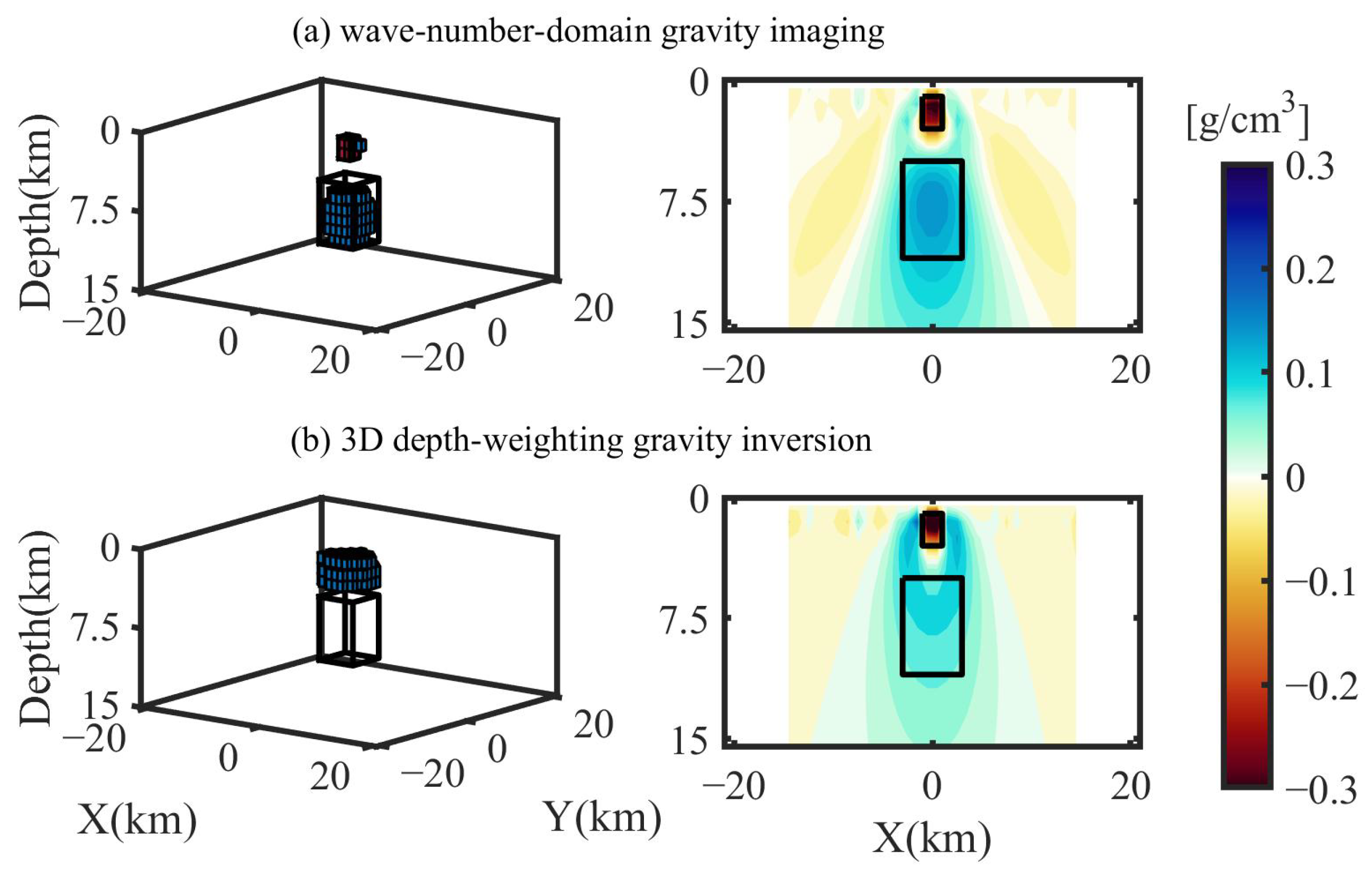Synthetic tests validate the effectiveness and robustness of the gravity and gradient imaging approaches, highlighting their advantages in high vertical resolution and low computational requirements. Nonetheless, it should be noted that the imaging effects of horizontal gradients ${\Gamma }_{xx}$ and ${\Gamma }_{yy}$ are unsatisfactory due to their weak noise resistance. 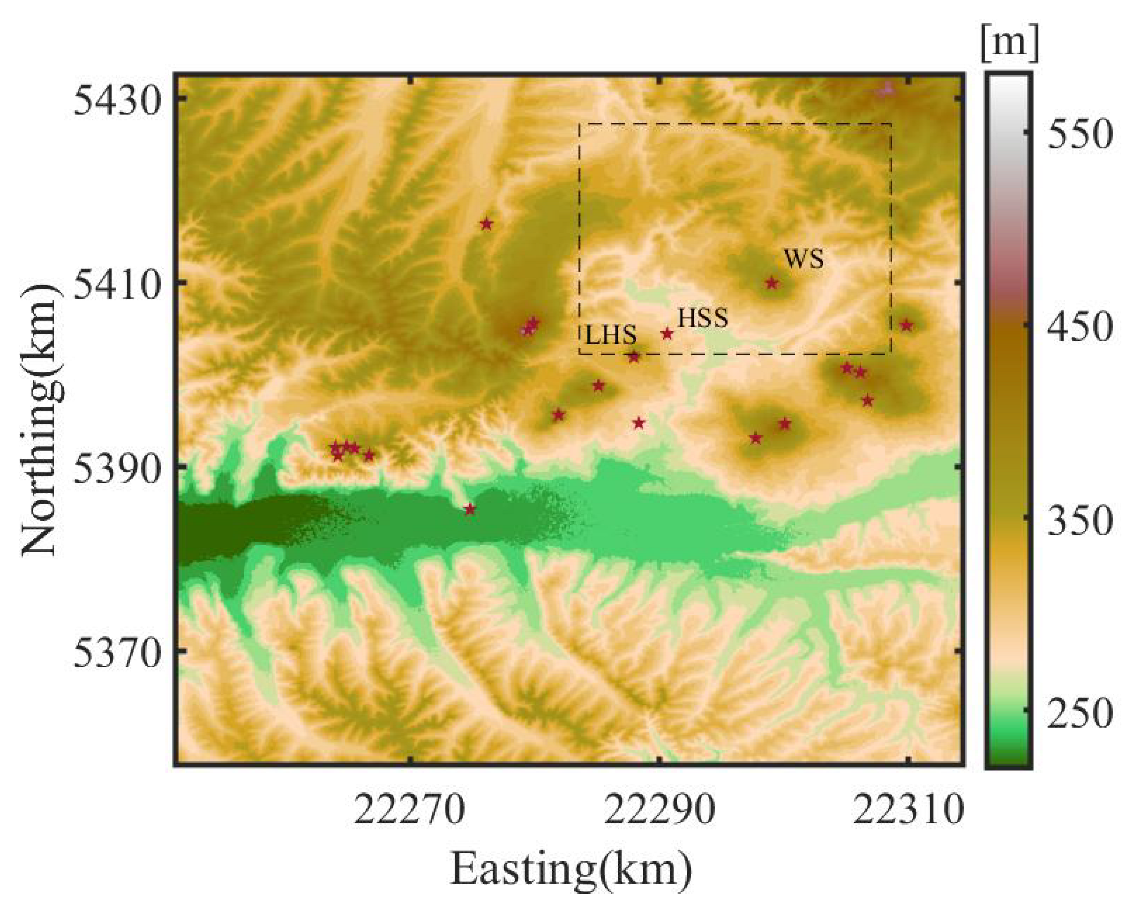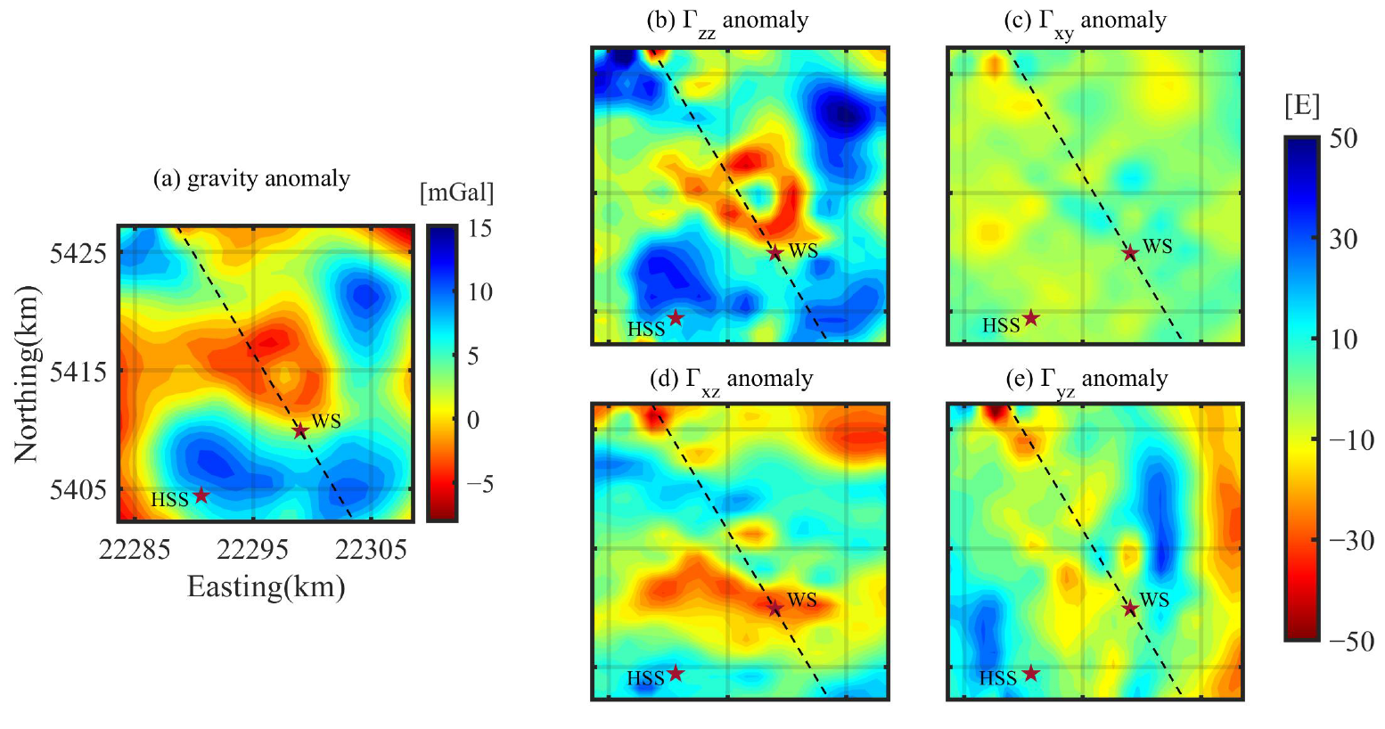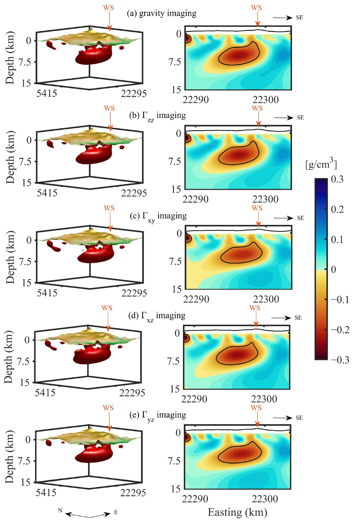Thus, they are not suitable for real data applications. The other imaging approaches are further applied to recover the subsurface 3D density structure beneath the Weishan cone in Wudalianchi Volcanic Field, Northeastern China. Our results provide insights into the possible location and shape of the low-density magma chamber. Also, the potential presence of partial melts is inferred and supported from a gravity perspective. The primary advantage of these approaches is their ability to generate a reasonable geological model in scenarios with limited prior information and physical property constraints. As a result, they have significant practical value in the field of applied geophysics, including mineral exploration and volcanology studies.

1. Introduction

The gravitational field is one of the fundamental geophysical fields. Apart from the contributions of the reference ellipsoid and topography relief on the geoid, the external residual gravity field mirrors the Earth’s interior heterogeneity [1]. Measurements of gravity and gradients, the first and second derivatives of gravitational potential, are common in geophysical surveying. Their anomalies or disturbances correlate with underground mass surplus/loss and can be applied in the modeling of density structure and undulating density interface [2,3,4,5,6,7].

Spatial three-dimensional (3D) inversion approaches are widely used to image the subsurface density distribution by gravity and gradients data. These approaches often incorporate linear regularization, whose constraints and weights are added to improve accuracy [8,9,10], such as depth-weighting inversion [11,12], focusing inversion [13,14,15], Lp-norm sparse inversion [16,17], Bayesian estimation [18], etc. Non-linear approaches, including the conjugate gradient method [19], the growing bodies method [20], simulated annealing [21], the genetic algorithm [22], and deep learning [23], have also been applied.

Additionally, the integrated 3D density imaging based on multi-scale field separation is an alternative approach. In contrast to direct inversion methods presented above, this approach offers advantages in improving the vertical resolution and computational efficiency. The spectral characteristics of gravity and magnetic fields are associated with the buried depth of field sources. Shallow source bodies typically manifest sharp local signals, while deep sources generally display broader, gradual signals. For targeted examination of particular geological structures, specific signals can be segregated through band-pass spatial filtering and following field imaging. Li and Oldenburg [24] developed a representative approach by applying wavelet transformation to simplify the computation of kernel matrices in 3D inversion, which was subsequently extended to facilitate multi-scale physical property inversion [25,26]. Mauriello and Patella [27] proposed the gravity probability tomography imaging approach to improve accuracy and mitigate non-uniqueness effects in gravity inversion. Concurrently, some studies also incorporated two-dimensional (2D) fast Fourier transformation (FFT) and Block–Toeplitz Toeplitz–Block (BTTB) matrix techniques [28,29] into forward modeling for similar purposes. Two-dimensional FFT deconvolution serves as a viable alternative to the matrix inverse process in solving linear equations, thereby enabling fast imaging with reduced computational burden [30,31,32]. Conventional field separation methods (e.g., wavelet analysis, matching filter, trend moving filter, and the cutting method) exhibit two primary limitations in the 3D imaging process. Firstly, the definitive relationship between separation scales and buried depth of mass layers remains elusive, which affects the accuracy of the imaging results. Secondly, the lack of integration between field separation and physical property imaging steps can introduce additional errors. In this study, we provide a novel strategy for gravitational field imaging by incorporating the preferential continuation filtering method. This strategy enables a direct transformation from planar field data to 3D density structures in the wave-number domain in a single step. The objective is to enhance the accurate and efficient identification of overlapping field sources while distinctly imaging complex subsurface density distributions and geological structures.

The continuation filter is a classical method for potential field separation [33]. By leveraging the low-pass filtering properties of upward continuation, different separation scales can be achieved by adjusting the continuation heights. It is capable of the 3D segmentation of 2D planar fields, leading to a more precise identification and localization of field sources at varying depths [34,35]. The preferential continuation is involved, which integrates analytical upward continuation and iterative downward continuation to establish a stable field separation operator in the wave-number domain, also aligning well with spectral density inversion techniques. With predefined grid parameters, our approaches facilitate the immediate generation of layered density distribution results using either gravity or gradient data inputs. To address the limitations of current inversion methods, we introduce the continuation repetition parameter and depth-scaling factor to optimize the density outcomes. While 3D gravity inversion theoretically poses non-uniqueness challenges, spatial inversion strategies often rely on prior knowledge or employ joint inversion methods. In cases where prior information is scarce, by our improved density-imaging strategy, adjusting the field separation effects through layered field imaging approaches can enhance the accuracy of the inversion results.

In recent years, advancements in gravity surveying techniques have led to the establishment of gravimeter and gradiometer test sites, one example being the Kauring Test Site in Australia [36]. In China, efforts are underway to develop the first airborne gravity gradiometer test site at the Wudalianchi Volcano National Geopark, primarily intended for calibrating and validating airborne gravimetric systems based on dense terrestrial gravity measurements as reported by Yang et al. [37]. The vast dataset collected from these tasks holds promise for various geophysical and geological interpretations. In this study, we utilize the high-resolution and high-accuracy terrestrial gravity data and generate them to planar gravity anomaly grids, as well as full-tensor gradient anomalies grids at flight altitudes. They will be employed to conduct real data tests of our density-imaging approaches.

The article is structured into five main sections. Section 2 introduces the fundamental mathematical theory underlying the preferential continuation filter and gravitational field imaging in the wave-number domain. Section 3 presents synthetic tests to assess the efficacy and robustness of our imaging approaches, highlighting their advantages in terms of low computational requirements and high vertical accuracy. In Section 4, we validate our approaches using real gravity and gradient data from the Wudalianchi test site, alongside discussions on the obtained density results. Finally, a concise conclusion is provided in Section 5.

2. Methodology

2.1. Preferential Continuation Filter

In potential field theory, the upward continuation typically functions as a spatial low-pass filter, while the downward continuation possesses the ability to enhance short wavelength field signals [38]. The preferential continuation filter, which integrates analytical upward continuation and iterative downward continuation, is employed for its superior performance in distinguishing short wavelength residual signals by eliminating long-wavelength regional signals. For a planar potential field U(x,y) at a reference height $z_0$, the corresponding field at a height h above is expressed as

$$F\left[U(x,y){|}_{z=z_0+h}\right]=e^{-kh}F\left[U(x,y){|}_{z=z_0}\right],$$

(1)

where $F[\cdots ]$ denotes the 2D Fourier transform operator, and $k=\sqrt{u^2+v^2}$ is the spatial wave number, where $u=2\pi f_x$ and $v=2\pi f_y$ with $f_x$ and $f_y$ represent the spatial frequencies in the x and y axes, respectively.

To achieve a stable downward continuation, some studies implemented an iterative strategy based on Taylor’s expansion to approximate the complete removal of noise and shallow-source signals [39,40,41]. In this study, respective Taylor’s series in the vertical and horizontal directions up to the second-order terms are considered, written as

$${U(x+\Delta x,y)|}_{z=z_0}={|U(x,y)+\frac{\partial U}{\partial x}\Delta x+\frac{1}{2}\frac{{\partial }^{2}U}{\partial x^2}\Delta x^2|}_{z=z_0},$$

(2)

$${U(x,y+\Delta y)|}_{z=z_0}={|U(x,y)+\frac{\partial U}{\partial y}\Delta y+\frac{1}{2}\frac{{\partial }^{2}U}{\partial y^2}\Delta y^2|}_{z=z_0},$$

(3)

$${U(x,y)|}_{z=z_0+\Delta z}={|U(x,y)+\frac{\partial U}{\partial z}\Delta z+\frac{1}{2}\frac{{\partial }^{2}U}{\partial z^2}\Delta z^2|}_{z=z_0}.$$

(4)

By substituting $\Delta x=\Delta y=\Delta z=\pm h$, the above three formulae sum to

$$\begin{array}{c}\hfill {U(x-h,y)|}_{z=z_0}{+U(x+h,y)|}_{z=z_0}+U(x,y-h){{|}_{z=z_0}+U(x,y+h)|}_{z=z_0}\\ \hfill {+U(x,y)|}_{z=z_0+h}{+U(x,y)|}_{z=z_0-h}=6U(x,y,z),\end{array}$$

(5)

where the sum of the second-order terms equals 0 in accordance with Laplace’s equation. The shifting property of Fourier transformation yields

$$F\left[U(x+h,y)\right]=2\pi e^{-iuh}F\left[U(x,y)\right],$$

(6)

$$F\left[U(x,y+h)\right]=2\pi e^{-ivh}F\left[U(x,y)\right].$$

(7)

Thus, Equation (5) can be reformulated as

$$\begin{array}{c}\hfill \left[2\pi \right(e^{iuh}+e^{-iuh}+e^{ivh}+e^{-ivh})+e^{-kh}]F\left[U(x,y){|}_{z=z_0}\right]\\ \hfill +F\left[U(x,y){|}_{z=z_0-h}\right]=6F\left[U(x,y,z)\right],\end{array}$$

(8)

and the spectral expression of downward continuation is deduced as

$$F\left[U(x,y){|}_{z=z_0-h}\right]=(6-e^{-kh}-2cosuh-2cosvh)F\left[U(x,y){|}_{z=z_0}\right].$$

(9)

The filtering effects of preferential continuation are controlled by the continuation height. Larger heights result in capturing longer wavelength signals. Let h denote the truncated height, and the deep-source field $U_d$ can be expressed as

$$F\left[U_d\right]=e^{-pkh}{(6-e^{-kh}-2cosuh-2cosvh)}^{p}F\left[U\right].$$

(10)

Here, p represents the repetition parameter, indicating the iteration count of the upward and downward continuation process crucial for ensuring convergence [42]. Quantities of the gravitational field, such as the gravitational potential, gravity vector, and gradient tensor, are applicable to such a field separation technique.

2.2. Wave-Number-Domain Density Imaging

In the context of gravitational field-density imaging, the band-pass field signals can be considered equivalent to the contribution of an underlying mass layer, which can further be transformed into a 2D density distribution. It is known as Green’s layer theory [43]. As shown in Figure 1, by segmenting the finite subsurface space into several layers and applying band-pass filtering to the corresponding field signals, an integrated 3D density structure can be modeled. For a space with n mass layers, the external gravitational field can be decomposed as

$$U=\sum _{l=1}^n\Delta U_l+U_0,$$

(11)

where $U_0$ represents the contribution from deep interior structures. The depths of the lower boundaries of each layer are denoted by $z_1<\cdots <z_n<0$. $\Delta U_l$, the response of the l-th mass layer, is extracted from the respective low-pass signals $\Delta U_{d,l+1}$ and $\Delta U_{d,l}$ with continuation heights $|z_{l+1}|$ and $|z_l|$ following Equation (10):

$$F[\Delta U_l]=F[\Delta U_{d,l+1}]-F[\Delta U_{d,l}].$$

(12)

Further, we establish the relationships between potential V, gravity vector

$$\mathbf{g}=\nabla V={[g_x,g_y,g_z]}^{\mathrm{T}},$$

(13)

gradient tensor

$$\mathbf{\Gamma }={\nabla }^{2}V=\left[\begin{array}{ccc}\delta {\Gamma }_{xx}& \delta {\Gamma }_{xy}& \delta {\Gamma }_{xz}\\ \delta {\Gamma }_{yx}& \delta {\Gamma }_{yy}& \delta {\Gamma }_{yz}\\ \delta {\Gamma }_{zx}& \delta {\Gamma }_{zy}& \delta {\Gamma }_{zz}\end{array}\right]$$

(14)

and density distribution in the wave-number domain.

In the Cartesian coordinate system, the disturbing potential response attracted by the l-th mass layer is mathematically formulated as [44]

$$\Delta V_l=\int {\int }_S{\int }_{z_l}^{z_{l+1}}\frac{{\rho }_l}{r}\mathrm{d}{z}^{\prime }\mathrm{d}{x}^{\prime }\mathrm{d}{y}^{\prime },$$

(15)

where G is the gravitational constant, ${\rho }_l$$(x^{\prime },y^{\prime })$ represents the planar density distribution, and $(x,y,z)$ are the coordinates of computation points, while $(x^{\prime },y^{\prime },z^{\prime })$ denote the integral elements. The distance between them is defined as

$$r=\sqrt{{(x-x^{\prime })}^2+{(y-y^{\prime })}^2+{(z-z^{\prime })}^2}.$$

(16)

Applying the definition formula of 2D Fourier transformation [45], Equation (15) can be reformulated as

$$\begin{array}{cc}\hfill F[\Delta V_l]& =\underset{-\infty }{\overset{\infty }{\int \int }}\Delta V_l{e}^{-i(ux+vy)}\mathrm{d}x\mathrm{d}y\hfill \\ \hfill & =G\underset{-\infty }{\overset{\infty }{\int \int }}{\rho }_l{e}^{-i(u{x}^{\prime }+v{y}^{\prime })}\mathrm{d}{x}^{\prime }\mathrm{d}{y}^{\prime }\times \hfill \\ \hfill & {\int }_{z_l}^{z_{l+1}}\underset{-\infty }{\overset{\infty }{\int \int }}\frac{1}{r}{e}^{-i[u(x-x^{\prime })+v(y-y^{\prime })]}\mathrm{d}(x-x^{\prime })\mathrm{d}(y-y^{\prime })\hfill \\ \hfill & =\frac{2\pi G}{k^2}(e^{-k|z-z_{l+1}|}-e^{-k|z-z_l|})F\left[{\rho }_l\right].\hfill \end{array}$$

(17)

However, the continuation height does not align precisely with the actual buried depth of the mass layer. Instead, there exists an approximate ratio between them, named the depth-scaling factor $\lambda$. Thus, Equation (17) is generalized to

$$F\left[V\right]=\sum _{l=1}^n\frac{2\pi G}{k^2}(e^{-k\lambda |z-z_{l+1}|}-e^{-k\lambda |z-z_l|})F\left[{\rho }_l\right],$$

(18)

and the expression of potential field separation is rewritten as

$$F[\Delta V_{d,l}]=e^{-pk\lambda |z_l|}{(6-e^{-k\lambda |z_l|}-2cosu\lambda |z_l|-2cosv\lambda |z_l|)}^{p}F\left[V\right],$$

(19)

which means the low-pass potential signals are truncated at continuation height $\lambda |z_l|$. Next, the stably separated potential $\Delta V_l$ can be continued downwards to the top of the mass layer to enhance the signals. The final expression of potential field imaging is written as

$$F\left[{\rho }_l\right]=\frac{k^2}{2\pi G}{(1-e^{k\lambda |z_{l+1}-z_l|})}^{-1}(6-e^{-k\lambda |z_l|}-2cosu\lambda |z_l|-2cosv\lambda |z_l|)F[\Delta V_l],$$

(20)

where $l=1,\cdots ,n$.

Equations (18) and (20) demonstrate the direct relationship between the external gravitational field and the interior density structure in the wave-number domain. It is also similar to the derivatives of potential. The respective relationships between the potential and its first and second derivatives are [38]

$$F\left[\mathbf{g}\right]=F[\nabla V]={[iu,iv,k]}^{\mathrm{T}}F\left[V\right],$$

(21)

and

$$F[\mathbf{\Gamma }]=F\left[{\nabla }^{2}V\right]=\left[\begin{array}{ccc}-u^2& -uv& iku\\ -uv& -v^2& ikv\\ iku& ikv& k^2\end{array}\right]F\left[V\right].$$

(22)

The derivatives of potential can also be stably separated by Equation (19), but there are slight changes in their forward and inverse expressions. We use the notation U as a common term in the gravitational field and generalize Equations (18) and (20) to

$$F\left[U\right]=\sum _{l=1}^{n}2\pi G(e^{-k\lambda |z-z_{l+1}|}-e^{-k\lambda |z-z_l|})F\left[{\rho }_l\right],$$

(23)

and

$$F\left[{\rho }_l\right]=\frac{1}{2\pi G}{(1-e^{k\lambda |z_{l+1}-z_l|})}^{-1}(6-e^{-kh}-2cosuh-2cosvh)F[\Delta U_l],$$

(24)

For potential,

$$U=k^{2}V,$$

(25)

for the components of gravity vector,

$$U=-\frac{i{k}^2}{u}{g}_x=-\frac{i{k}^2}{v}{g}_y=k{g}_z,$$

(26)

and for the components of gradient tensor,

$$\begin{array}{cc}\hfill U& =-\frac{k^2}{u^2}{\Gamma }_{xx}=-\frac{k^2}{v^2}{\Gamma }_{yy}={\Gamma }_{zz}\hfill \\ \hfill & =-\frac{k^2}{uv}{\Gamma }_{xy}=-\frac{ik}{u}{\Gamma }_{xz}=-\frac{ik}{v}{\Gamma }_{yz}.\hfill \end{array}$$

(27)

Using these 3D imaging approaches based on gravitational field separation, the problems of skin effects and overlapping field sources can be better addressed. Still, the imaging results of source bodies may be vertically shifted. They can be refined by adjusting appropriate parameters p and $\lambda$. In practice, the optimal parameters are determined through trial and error, with details provided in the next section.

3. Synthetic Tests

To validate the performance of our improved approaches, two synthetic model tests are designed. Model I consists of two parallel cubes as shown in Figure 2a. The deep cube is centered at (−3, −3, −8) km with equal sides of 6 km and a density of 1.0 g/cm³. The shallow cube is centered at (6.5, 6.5, −4.5) km with equal sides of 3 km and a density of −1.0 g/cm³. The distribution of gravity and full-tensor gradient observations at the reference surface ($z=0$ km) are also shown in Figure 2. The inversion tests are conducted in a $40\times 40\times 15$ km³ ($x\times y\times z$ dimensions) subsurface space. The thickness of all mass layers and the horizontal grid size in both the x and y axes are set to 1.0 km. The simulated inversion results are illustrated through density profiles and 3D perspective views. The former are along the dashed lines in Figure 2 and the latter are with a truncated density of ±0.13 g/cm³.

The inversion effects are determined by the repetition parameter p and the depth scaling factor $\lambda$. With regard to the repetition parameter, it not only controls the degree of completeness in field separation but also exerts an influence on the field-imaging process. As an example, a comparison among the gravity-imaging results with a fixed $\lambda$ value of 0.4 and three different p values ($p=$ 5, 20, 50) is made. As shown in Figure 3a–c, an increase in the p value leads to a change that two source bodies manifest a vertically shortened shape and a shallower buried depth. This is likely due to the fact that a greater number iteration in the continuation process can amplify short-wavelength signals and attenuate long-wavelength signals. The imaging results with a fixed p value of 30 and three different $\lambda$ values ($\lambda =$ 0.25, 0.35, 0.45) are compared, exhibiting the same change in the source bodies with decreasing $\lambda$ as shown in Figure 3d–f. Figure 3b,e indicate that different combinations of p and $\lambda$ can yield similar imaging results that closely resemble the model. We compile these parameter sets and present an “L” shaped curve shown in Figure 4. It is observed that with larger p and smaller $\lambda$ values, the residual error of the corresponding solution decreases while the standard variation increases. And the inflection point of the L-curve can be selected to determine the optimal solution, with the parameters $p=40$ and $\lambda =0.33$. Additional tests are conducted to explore the L-curve characteristics of various gravity-imaging results, all of which give the same optimal parameters, including the Model II test and applications discussed below. Consequently, it can be inferred that p and $\lambda$ are intrinsic parameters independent of the input data. However, the gradient imaging results do not display an L-curve relation but a positive correlation between their residual errors and standard variations. Nonetheless, as shown in Figure 5, exceptional solutions can still be achieved with $p=40$ and $\lambda =0.33$, which are regarded equivalent to the optimal parameters for gradients.

The results of gravity and ${\Gamma }_{zz}$, ${\Gamma }_{xy}$, ${\Gamma }_{xz}$, ${\Gamma }_{yz}$ gradient imaging in Figure 5a,d–g reveal superior effects in strong noise immunity and precise vertical focusing of source bodies. However, the results of ${\Gamma }_{xx}$ and ${\Gamma }_{yy}$ gradient imaging in Figure 5b,c indicate comparatively inferior performance, attributed to weaker noise immunity and larger boundary effects. To specifically investigate the robustness of these imaging approaches, a comparative analysis at various noise levels is taken. Based on the simulated gravity and ${\Gamma }_{xx}$, ${\Gamma }_{yy}$, and ${\Gamma }_{zz}$ gradient observations in Figure 2, four scenarios—no noise, 2%, 5%, and 20% Gaussian white noise added—are considered, respectively. Density profiles of the corresponding imaging results are shown in Figure 6. In the absence of additional noise, ${\Gamma }_{xx}$ and ${\Gamma }_{yy}$ gradient imaging also show perfect performance. But introducing even minor noise can lead to interference of the imaging results, potentially obscuring field sources at depths shallower than 3 km. If the noise level exceeds a specific threshold, the imaging process becomes unfeasible. In comparison, gravity and ${\Gamma }_{zz}$ gradient imaging exhibit superior robustness. At a noise level of 20%, interference emerges in the gravity-imaging results, while ${\Gamma }_{zz}$ imaging results remain stable. The limited noise suppression capability of the ${\Gamma }_{xx}$ and ${\Gamma }_{yy}$ imaging processes renders them unsuitable for real data applications.

Model II consists of two vertically overlapping blocks as shown in Figure 7a. The deep one is a cube centered at (0, 0, −8) km with equal sides of 6 km and a density of 1.0 g/cm³. The shallow cube is centered at (0, 0, −2) km with equal sides of 2 km and a density of −1.0 g/cm³. The distribution of gravity and full-tensor gradient observations are also shown in Figure 7. Simulated imaging tests are conducted in the $40\times 40\times 15$ km³ subsurface space, with the grid size and inversion parameters being identical to those of Model I. Gravity and full-tensor gradient imaging results, as shown in Figure 8 and Figure 9a, illustrate the effectiveness of the improved imaging approaches in accurately recovering the shape and position of vertically overlapping sources from the mixed field signals. Nonetheless, it should be noted that the interference from the field signals of deep and shallow sources cannot be entirely eliminated. This results in distortion in the shallow, characterized by the presence of some high-density anomalies surrounding the central low-density body.

Additionally, we provide a comparison of our improved gravity-imaging approach with other commonly used gravity inversion methods. The basic principle of 3D gravity inversion is solving the linear equation in the matrix-vector form based on the relationship between density and gravity anomaly. An optimal solution that minimizes the objective function can be obtained. This process is the so-called Tikhonov regularization [46]. In order to improve the vertical accuracy of the inversion results, Li and Oldenburg [11] introduced the depth weighting process, which is widely applied at present [3,6,47]. There are significant differences in computational efficiency and inversion performance between the depth-weighting gravity inversion and our wave-number-domain gravity-imaging approaches. The regular inversion process involves considerable time in kernel matrix construction and regularization. In contrast, wave-number-domain imaging utilizes the FFT technique, which only requires matrix dot-product calculation. As an example of the simulated inversion of Model II, a simple test on computation time and data storage associated with these two approaches is carried out, using the MATLAB 2020a language version on a laptop equipped with an Intel(R) Core(TM) i7-10510U CPU. With a setting of $30\times 30\times 15$ grids in density inversion and 900 gravity anomaly observation points, the kernel matrix is sized at 900 × 13,500. The forward calculation takes a time of 283 s, and 38 s are spent in the regularization process, occupying a total physical memory of 2311 MB. However, the whole wave-number-domain imaging process just takes a time of 0.2 s and occupies a physical memory of only 94 MB. This indicates that the matrix construction and inverse operation can be replaced by a more efficient way like convolution and deconvolution in the frequency domain. The reduced computational requirements also facilitate the recovery of more detailed density structures. The inversion results of the two approaches are shown in Figure 9. In comparison, although the depth weighting inversion method can identify shallow and deep sources, the deep one is significantly distorted, and its buried depth is also inaccurate. The wave-number-domain imaging approaches exhibit relatively superior ability in identifying vertically overlapping field sources and have greater advantages in applications under complex geological conditions.

4. Applications

The terrestrial or airborne gravity and gradient anomalies serve as essential indicators of the dense and sparse distribution of subsurface materials. Gravity field imaging approaches can be effectively applied to investigate local density anomalies, such as oil and gas reservoirs, metal deposits, magma chambers, etc. [48,49,50]. To validate our improved approaches applied to real gravity and gradient data, we select the near zone of the Weishan volcanic cone in the Wudalianchi region as the study area as shown in Figure 10. The Wudalianchi Volcanic Field, a representative Cenozoic volcano in Northeastern China, is situated at the junction of the northern edge of Songliao Basin and the Lesser Xing’an Range. It encompasses an area of more than 800 km² with several monogenetic volcanic cones, and it is characterized by potassium-rich basalts [51,52,53]. The most recent recorded eruptions, occurred at Laoheishan and Huoshaoshan cones in 1719–1721, suggest the potential for ongoing volcanic activity. The latest geophysical surveys in Wudalianchi region indicate the possible presence of incompletely cooled magma chambers, with specific attention towards the Weishan area [54,55,56]. In gravity field observations, magma chambers are associated with distinct negative anomaly features, due to the relatively low density of basalt in relation to the average density of the upper crust. This enables the density imaging of magma chambers and their related structures.

The terrestrial gravimetric data applied in this study are from the gravity survey of the Wudalianchi airborne gravity gradiometer test site. The residual Bouguer gravity anomalies are derived by reducing long-wavelength signals and residual topographic effects, and the corresponding ${\Gamma }_{zz}$, ${\Gamma }_{xy}$, ${\Gamma }_{xz}$, and ${\Gamma }_{yz}$ gradient anomalies are then transformed by the least-square collocation method. Gravity and gradient anomalies in the study area are gridded to a resolution of $1\times 1$ km and reduced to an altitude of 500 m, as shown in Figure 11. Also, these data are applied in 3D density imaging using our improved approaches. The horizontal density grid size is consistent with the observation grid, and the mass layer thickness is set to 0.5 km. The maximum imaging depth is set to 15 km. The values of the repetition parameter p and depth scaling factor $\lambda$ are the same as those used in model tests, i.e., $p=40$ and $\lambda =0.33$. Density-imaging results are shown in Figure 12. Density anomalies range within ±0.3 g/cm3, and we select −0.1 g/cm³ as the truncation value to generate 3D perspective views. Also, depth profiles are taken along the line connecting Huoshaoshan and Weishan (in the SW-NE direction).

As shown in Figure 10, volcanic cones are mainly arranged along three SW-NE alignments. The Weishan cone is located at the northeast of the central alignment. The topography of the Weishan area exhibits a typical volcanic dome formation, probably attributed to the ascent of deep melts. Bouguer gravity and ${\Gamma }_{zz}$ gradient anomalies in the study area (Figure 11a) show a negative feature near the Weishan cone. From a petrological perspective, the negative features reflect low-density basalts or basaltic magma, and the positive features reflect high-density basement metamorphic rocks [55]. However, the cone is not positioned at the focal point of the negative feature but rather at the southeastern juncture of the positive and negative features. As shown in Figure 12, the gravity and gradient imaging results all reveal a low-density chamber with a buried depth ranging from about 3 to 8 km, and a channel-like structure originates from the chamber, extends southeastward, and links to the Weishan cone.

Seismic and magnetotelluric surveys were also previously conducted in this area. Li et al. [54] employed the ambient noise tomography to find a low-velocity anomaly beneath Weishan at a depth of about 7–13 km. Gao et al. [56] identified two low-resistivity anomalies above and below 8 km in depth through magnetotelluric imaging, and inferred that the magma chamber might be in the “recharging” state. Yet, Sun et al. [57] contended that the low-resistivity bodies could also be attributed to saline fluids rather than partial melts. The low-density chamber revealed in this study could correspond to such low-velocity and low-resistivity anomalies. From a petrological perspective, the basement metamorphic rocks exhibit a density exceeding 2.8 g/cm³, whereas the density of basalts is below 2.4 g/cm³. The significant contrast in density is consistent with our density-imaging results. We speculate that the low-density anomaly probably represents a remnant magmatic structure from the last eruption of Weishan. Combined with the low-velocity, low-resistivity and low-density characteristics, it is plausible that the chamber still contains basaltic partial melts. In general, the real data tests validate the better performance of our gravity field imaging approaches in identifying the position and shape of geological bodies with distinctive densities.

5. Conclusions and Outlooks

In this study, we introduce the preferential continuation filtering technique and develop the improved 3D gravity and full-tensor gradient imaging approaches based on field separation in the wave-number domain. Synthetic tests validate the effectiveness and noise resistance of our imaging approaches. Specifically, they demonstrate the ability to identify and separate vertically overlapping sources, notably improving the vertical resolution of inversion results and effectively addressing the skin effects than the depth-weighting gravity inversion methods. Another advantage is their high computational efficiency without compromising inversion accuracy. This makes it easier to recover more detailed density structures in practice with a comparatively low computation burden. Still, some limitations should be also mentioned. The imaging approaches are only suitable for the processed planar gridding field data, which is comparatively less convenient than regularization methods. And these approaches are inapplicable to inversion scenarios with strict constraints in shape, buried depth, or density values. For ${\Gamma }_{xx}$ and ${\Gamma }_{yy}$ gradient imaging, their noise resistance is relatively poor, impacting the imaging quality of near-surface shallow field sources.

The applications in Wudalianchi Volcanic Field confirm the practicability of gravity and ${\Gamma }_{zz}$, ${\Gamma }_{xy}$, ${\Gamma }_{xz}$, ${\Gamma }_{yz}$ gradient imaging approaches in complex geological study areas. Utilizing Bouguer gravity anomaly and the corresponding gradient anomalies, the subsurface density imaging of Weishan area at depths shallower than 15 km is performed. A low-density chamber-like body is found to the northwest of the Weishan cone, with a buried depth shallower than 10 km. The identification of low-velocity anomalies in previous seismic studies and low-resistivity anomalies in magnetotelluric studies, along with the gravity-imaging results in this study, provides further evidence for the potential existence of partial melts in the magma chamber.

Overall, despite the theoretical non-uniqueness of gravity inversion, our approaches prove to be useful with limited prior information and physical property constraints. With only gravity or gradient field observations, an initial underground geological model can be created, based on the mathematical constraints of the spectral characteristics of the potential field and the size and buried depth of the geological features. These preliminary results provide references for subsequent geological and geophysical research. Such a density-imaging strategy can be highly beneficial in mineral exploration and volcanology applications.

References

- Hofmann-Wellenhof, B.; Morisz, H. Physical Geodesy; Springer: Wien, Austria, 2005. [Google Scholar]
- Braitenberg, C.; Zadro, M.; Fang, J.; Wang, Y.; Hsu, H. The gravity and isostatic Moho undulations in Qinghai–Tibet plateau. J. Geodyn. 2000, 30, 489–505. [Google Scholar] [CrossRef]
- Li, Y.; Yang, Y. Gravity data inversion for the lithospheric density structure beneath North China Craton from EGM 2008 model. Phys. Earth Planet. Inter. 2011, 189, 9–26. [Google Scholar] [CrossRef]
- Motavalli-Anbaran, S.H.; Zeyen, H.; Ebrahimzadeh Ardestani, V. 3D joint inversion modeling of the lithospheric density structure based on gravity, geoid and topography data—Application to the Alborz Mountains (Iran) and South Caspian Basin region. Tectonophysics 2013, 586, 192–205. [Google Scholar] [CrossRef]
- Yang, W.; Chen, Z.; Hou, Z.; Yu, C. Three Dimensional Crustal Density Structure of Central Asia and its Geological Implications. Acta Geophys. 2016, 64, 1257–1274. [Google Scholar] [CrossRef]
- Tian, Y.; Li, H.; Wang, Y.; Ye, Q.; Guo, A. Gravity Gradient Inversion of Gravity Field and Steady-State Ocean Circulation Explorer Satellite Data for the Lithospheric Density Structure in the Qinghai-Tibet Plateau Region and the Surrounding Regions. J. Geophys. Res. Solid Earth 2021, 126, e2020JB021291. [Google Scholar] [CrossRef]
- Haas, P.; Ebbing, J.; Szwillus, W. Cratonic crust illuminated by global gravity gradient inversion. Gondwana Res. 2023, 121, 276–292. [Google Scholar] [CrossRef]
- Bear, G.W.; Al-Shukri, H.J.; Rudman, A.J. Linear inversion of gravity data for 3-D density distributions. Geophysics 1995, 60, 1354–1364. [Google Scholar] [CrossRef]
- Boulanger, O.; Chouteau, M. Constraints in 3D gravity inversion. Geophys. Prospect. 2001, 49, 265–280. [Google Scholar] [CrossRef]
- Pilkington, M. Analysis of gravity gradiometer inverse problems using optimal design measures. Geophysics 2012, 77, G25–G31. [Google Scholar] [CrossRef]
- Li, Y.; Oldenburg, D.W. 3-D inversion of gravity data. Geophysics 1998, 63, 109–119. [Google Scholar] [CrossRef]
- Li, Y. 3-D inversion of gravity gradiometer data. In SEG Technical Program Expanded Abstracts; Society of Exploration Geophysicists: San Antonio, TX, USA, 2001; pp. 1470–1473. [Google Scholar] [CrossRef]
- Portniaguine, O.; Zhdanov, M.S. Focusing geophysical inversion images. Geophysics 1999, 64, 659–992. [Google Scholar] [CrossRef]
- Zhdanov, M.S.; Ellis, R.; Mukherjee, S. Three-dimensional regularized focusing inversion of gravity gradient tensor component data. Geophysics 2004, 69, 877–1103. [Google Scholar] [CrossRef]
- Ma, G.; Wang, T.; Meng, Q.; Li, Z.; Wang, T.; Li, L. 3-D inversion of gravity anomalies by combining power-spectrum derived adaptive weighting and cross-gradient regulation: Application to Molybdenum–Copper deposit. IEEE Trans. Geosci. Remote. Sens. 2022, 60, 1–9. [Google Scholar] [CrossRef]
- Meng, Z. 3D inversion of full gravity gradient tensor data using SL0 sparse recovery. J. Appl. Geophys. 2016, 127, 112–128. [Google Scholar] [CrossRef]
- Li, Z.; Yao, C.; Zheng, Y. 3D inversion of gravity data using Lp-norm sparse optimization. Chin. J. Geophys. 2019, 62, 3699–3709. [Google Scholar] [CrossRef]
- Calvetti, D.; Somersalo, E. Inverse problems: From regularization to Bayesian inference. WIREs Comput. Stat. 2018, 10, e1427. [Google Scholar] [CrossRef]
- Qin, P.; Huang, D.; Yuan, Y.; Geng, M.; Liu, J. Integrated gravity and gravity gradient 3D inversion using the non-linear conjugate gradient. J. Appl. Geophys. 2016, 126, 52–73. [Google Scholar] [CrossRef]
- Camacho, A.G.; Montesinos, F.G.; Vieira, R. Gravity inversion by means of growing bodies. Geophysics 2000, 65, 95–101. [Google Scholar] [CrossRef]
- Nagihara, S.; Hall, S.A. Three-dimensional gravity inversion using simulated annealing: Constraints on the diapiric roots of allochthonous salt structures. Geophysics 2001, 66, 1438–1449. [Google Scholar] [CrossRef]
- Montesinos, F.G.; Arnoso, J.; Vieira, R. Using a genetic algorithm for 3-D inversion of gravity data in Fuerteventura (Canary Islands). Int. J. Earth Sci. 2005, 94, 301–316. [Google Scholar] [CrossRef]
- Zhang, L.; Zhang, G.; Liu, Y.; Fan, Z. Deep Learning for 3-D Inversion of Gravity Data. IEEE Trans. Geosci. Remote Sens. 2022, 60, 1–18. [Google Scholar] [CrossRef]
- Li, Y.; Oldenburg, D.W. Fast inversion of large-scale magnetic data using wavelet transforms and a logarithmic barrier method. Geophys. J. Int. 2003, 152, 251–265. [Google Scholar] [CrossRef]
- Davis, K.; Li, Y. Fast solution of geophysical inversion using adaptive mesh, space-filling curves and wavelet compression. Geophys. J. Int. 2011, 185, 157–166. [Google Scholar] [CrossRef]
- Sun, S.Y.; Yin, C.C.; Gao, X.H.; Liu, Y.H.; Ren, X.Y. Gravity compression forward modeling and multiscale inversion based on wavelet transform. Appl. Geophys. 2018, 15, 342–352. [Google Scholar] [CrossRef]
- Mauriello, P.; Patella, D. Gravity probability tomography: A new tool for buried mass distribution imaging. Geophys. Prospect. 2001, 49, 1–12. [Google Scholar] [CrossRef]
- Zhang, Y.; Wong, Y.S. BTTB-based numerical schemes for three-dimensional gravity field inversion. Geophys. J. Int. 2015, 203, 243–256. [Google Scholar] [CrossRef]
- Renaut, R.A.; Hogue, J.D.; Vatankhah, S.; Liu, S. A fast methodology for large-scale focusing inversion of gravity and magnetic data using the structured model matrix and the 2-D fast Fourier transform. Geophys. J. Int. 2020, 223, 1378–1397. [Google Scholar] [CrossRef]
- Xu, S.; Yu, H.; Li, H.; Tian, G.; Yang, J. The inversion of apparent density based on the separation and continuation of potential field. Chin. J. Geophys. 2009, 52, 1592–1598. (In Chinese) [Google Scholar] [CrossRef]
- Cui, Y.; Guo, L. A wavenumber-domain iterative approach for rapid 3-D imaging of gravity anomalies and gradients. IEEE Access 2019, 7, 34179–34188. [Google Scholar] [CrossRef]
- Qiang, J.; Xu, J.; Lu, K.; Guo, Z. A Fast Forward and Inversion Strategy for Three-Dimensional Gravity Field. Mathematics 2023, 11, 962. [Google Scholar] [CrossRef]
- Pawlowski, R.S. Preferential continuation for potential-field anomaly enhancement. Geophysics 1995, 60, 390–398. [Google Scholar] [CrossRef]
- Meng, X.; Guo, L.; Chen, Z.; Li, S.; Shi, L. A method for gravity anomaly separation based on preferential continuation and its application. Appl. Geophys. 2009, 6, 217–225. [Google Scholar] [CrossRef]
- Guo, L.; Meng, X.; Chen, Z.; Li, S.; Zheng, Y. Preferential filtering for gravity anomaly separation. Comput. Geosci. 2013, 51, 247–254. [Google Scholar] [CrossRef]
- Christensen, A.N. Results from FALCON Airborne Gravity Gradiometer surveys over the Kauring AGG Test site. In Proceedings of the 23rd ASEG-PESA International Geophysical Conference and Exhibition, ASEG Extended Abstracts, Melbourne, Australia, 11–14 August 2013; pp. 1–4. [Google Scholar] [CrossRef]
- Yang, M.; Li, W.K.; Feng, W.; Pail, R.; Wu, Y.G.; Zhong, M. Integration of Residual Terrain Modelling and the Equivalent Source Layer Method in Gravity Field Synthesis for Airborne Gravity Gradiometer Test Site Determination. Remote Sens. 2023, 15, 5190. [Google Scholar] [CrossRef]
- Blakely, R. Potential Theory in Gravity and Magnetic Applications; Cambridge University Press: New York, NY, USA, 1995. [Google Scholar]
- Fedi, M.; Florio, G. A stable downward continuation by using the ISVD method. Geophys. J. Int. 2002, 151, 146–156. [Google Scholar] [CrossRef]
- Florio, G.; Fedi, M.; Pasteka, R. On the application of Euler deconvolution to the analytic signal. Geophysics 2006, 71, L87–L93. [Google Scholar] [CrossRef]
- Ma, G.; Liu, C.; Huang, D.; Li, L. A stable iterative downward continuation of potential field data. J. Appl. Geophys. 2013, 98, 205–211. [Google Scholar] [CrossRef]
- Xu, S.; Yang, J.; Yang, C.; Xiao, P.; Chen, S.; Guo, Z. The iteration method for downward continuation of a potential field from a horizontal plane. Geophys. Prospect. 2007, 55, 883–889. [Google Scholar] [CrossRef]
- Pawlowski, R.S. Green’s equivalent-layer concept in gravity band-pass filter design. Geophysics 1994, 59, 69–76. [Google Scholar] [CrossRef]
- Nagy, D.; Papp, G.; Benedek, J. The gravitational potential and its derivatives for the prism. J. Geod. 2000, 74, 552–560. [Google Scholar] [CrossRef]
- Parker, R. The rapid calculation of potential anomalies. Geophys. J. Res. Astron. Soc. 1972, 31, 447–455. [Google Scholar] [CrossRef]
- Tikhonov, A.N. Solution of Incorrectly Formulated Problems and the Regularization Method. Sov. Math. Dokl. 1963, 4, 1035–1038. [Google Scholar]
- Ghari, H.; Varfinezhad, R.; Parnow, S. 3D joint interpretation of potential field, geology, and well data to evaluate a salt dome in the Qarah-Aghaje area, Zanjan, NW Iran. Near Surf. Geophys. 2023, 21, 233–246. [Google Scholar] [CrossRef]
- Deng, F.; Connor, C.B.; Malservisi, R.; Connor, L.J.; White, J.T.; Germa, A.; Wetmore, P.H. A Geophysical Model for the Origin of Volcano Vent Clusters in a Colorado Plateau Volcanic Field. J. Geophys. Res. Solid Earth 2017, 122, 8910–8924. [Google Scholar] [CrossRef]
- Miller, C.A.; Williams-Jones, G.; Fournier, D.; Witter, J. 3D gravity inversion and thermodynamic modelling reveal properties of shallow silicic magma reservoir beneath Laguna del Maule, Chile. Earth Planet. Sci. Lett. 2017, 459, 14–27. [Google Scholar] [CrossRef]
- Zhang, M.; Qiao, J.; Zhao, G.; Lan, X. Regional gravity survey and application in oil and gas exploration in China. China Geol. 2019, 2, 382–390. [Google Scholar] [CrossRef]
- Shao, J.; Zhang, W. The evolving rift belt-Wudalianchi volcanic rock belt. Earth Sci. Front. 2008, 15, 241–250. (In Chinese) [Google Scholar]
- Zhao, Y.W.; Li, N.; Fan, Q.C.; Zou, H.; Xu, Y.G. Two episodes of volcanism in the Wudalianchi volcanic belt, NE China: Evidence for tectonic controls on volcanic activities. J. Volcanol. Geotherm. Res. 2014, 285, 170–179. [Google Scholar] [CrossRef]
- Rasskazov, S.V.; Chuvashova, I.S.; Sun, Y.m.; Yang, C.; Xie, Z.; Yasnygina, T.A.; Saranina, E.V.; Fang, Z. Sources of Quaternary Potassic Volcanic Rocks from Wudalianchi, China: Control by Transtension at the Lithosphere–Asthenosphere Boundary Layer. Geodyn. Tectonophys. 2016, 7, 555–592. [Google Scholar] [CrossRef]
- Li, Z.; Ni, S.; Zhang, B.; Bao, F.; Zhang, S.; Deng, Y.; Yuen, D.A. Shallow magma chamber under the Wudalianchi Volcanic Field unveiled by seismic imaging with dense array. Geophys. Res. Lett. 2016, 43, 4954–4961. [Google Scholar] [CrossRef]
- Zhang, S.; Jia, X.; Zhang, Y.; Li, S.; Li, Z.; Tian, P.; Ming, Y.; Zhang, C. Volcanic magma chamber survey and geothermal geological condition analysis for hot dry rock at the Weishan Volcano in Wudalianchi Region, Heilongjinag Province. Acta Geol. Sin. 2017, 91, 1–16. (In Chinese) [Google Scholar]
- Gao, J.; Zhang, H.; Zhang, S.; Xin, H.; Li, Z.; Tian, W.; Bao, F.; Cheng, Z.; Jia, X.; Fu, L. Magma recharging beneath the Weishan volcano of the intraplate Wudalianchi volcanic field, northeast China, implied from 3-D magnetotelluric imaging. Geology 2020, 48, 913–918. [Google Scholar] [CrossRef]
- Sun, X.; Zhan, Y.; Zhao, L.; Xu, J.; Zhao, Y.; Zhao, B.; Yang, W. Does a Shallow Magma Reservoir Exist in the Wudalianchi Volcanic Field? Constraints From Magnetotelluric Imaging. Geophys. Res. Lett. 2023, 50, e2023GL104318. [Google Scholar] [CrossRef]
Disclaimer/Publisher’s Note: The statements, opinions and data contained in all publications are solely those of the individual author(s) and contributor(s) and not of MDPI and/or the editor(s). MDPI and/or the editor(s) disclaim responsibility for any injury to people or property resulting from any ideas, methods, instructions or products referred to in the content. |
© 2024 by the authors. Licensee MDPI, Basel, Switzerland. This article is an open access article distributed under the terms and conditions of the Creative Commons Attribution (CC BY) license (https://creativecommons.org/licenses/by/4.0/).
Share and Cite
Li, W.; Yang, M.; Feng, W.; Zhong, M. Improved Approaches for 3D Gravity and Gradient Imaging Based on Potential Field Separation: Application to the Magma Chamber in Wudalianchi Volcanic Field, Northeastern China. Remote Sens. 2024, 16, 1187. https://doi.org/10.3390/rs16071187
Li W, Yang M, Feng W, Zhong M. Improved Approaches for 3D Gravity and Gradient Imaging Based on Potential Field Separation: Application to the Magma Chamber in Wudalianchi Volcanic Field, Northeastern China. Remote Sensing. 2024; 16(7):1187. https://doi.org/10.3390/rs16071187
Chicago/Turabian StyleLi, Weikai, Meng Yang, Wei Feng, and Min Zhong. 2024. "Improved Approaches for 3D Gravity and Gradient Imaging Based on Potential Field Separation: Application to the Magma Chamber in Wudalianchi Volcanic Field, Northeastern China" Remote Sensing 16, no. 7: 1187. https://doi.org/10.3390/rs16071187