

A Regional Aerosol Model for the Oceanic Area around Eastern China Based on Aerosol Robotic Network (AERONET)
 , , , and
Abstract
:
1. Introduction
2. Data and Method
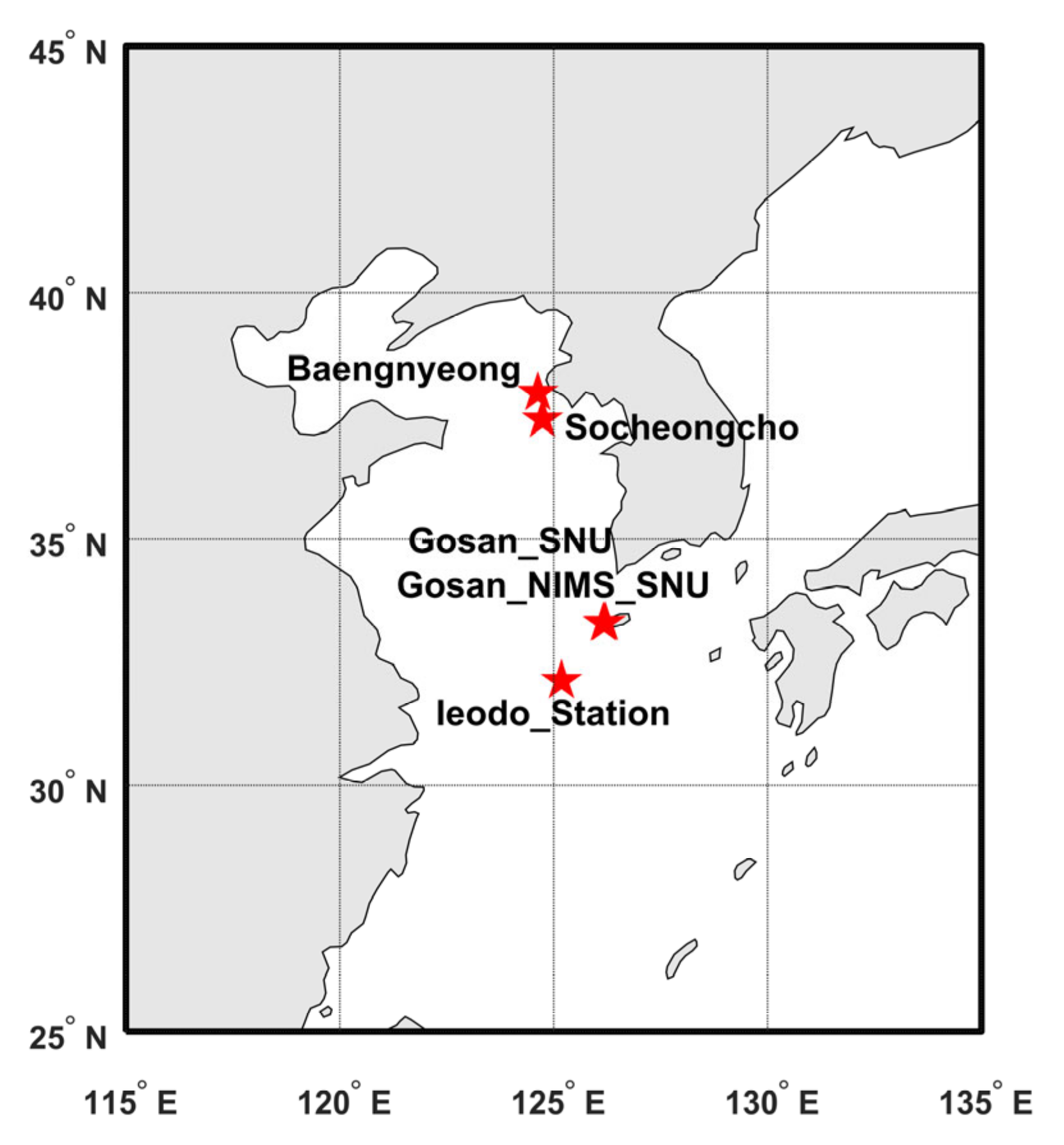
2.1. AERONET Data
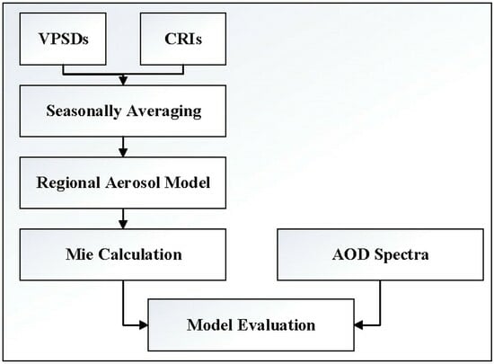
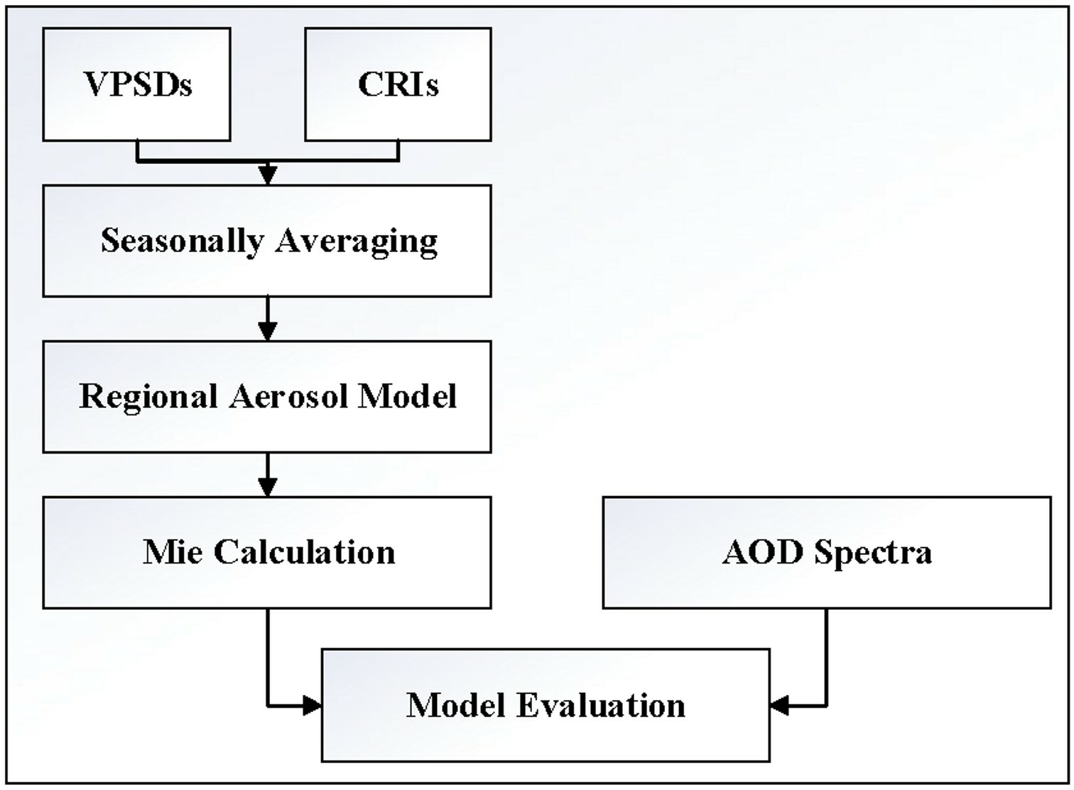
2.2. Aerosol Model
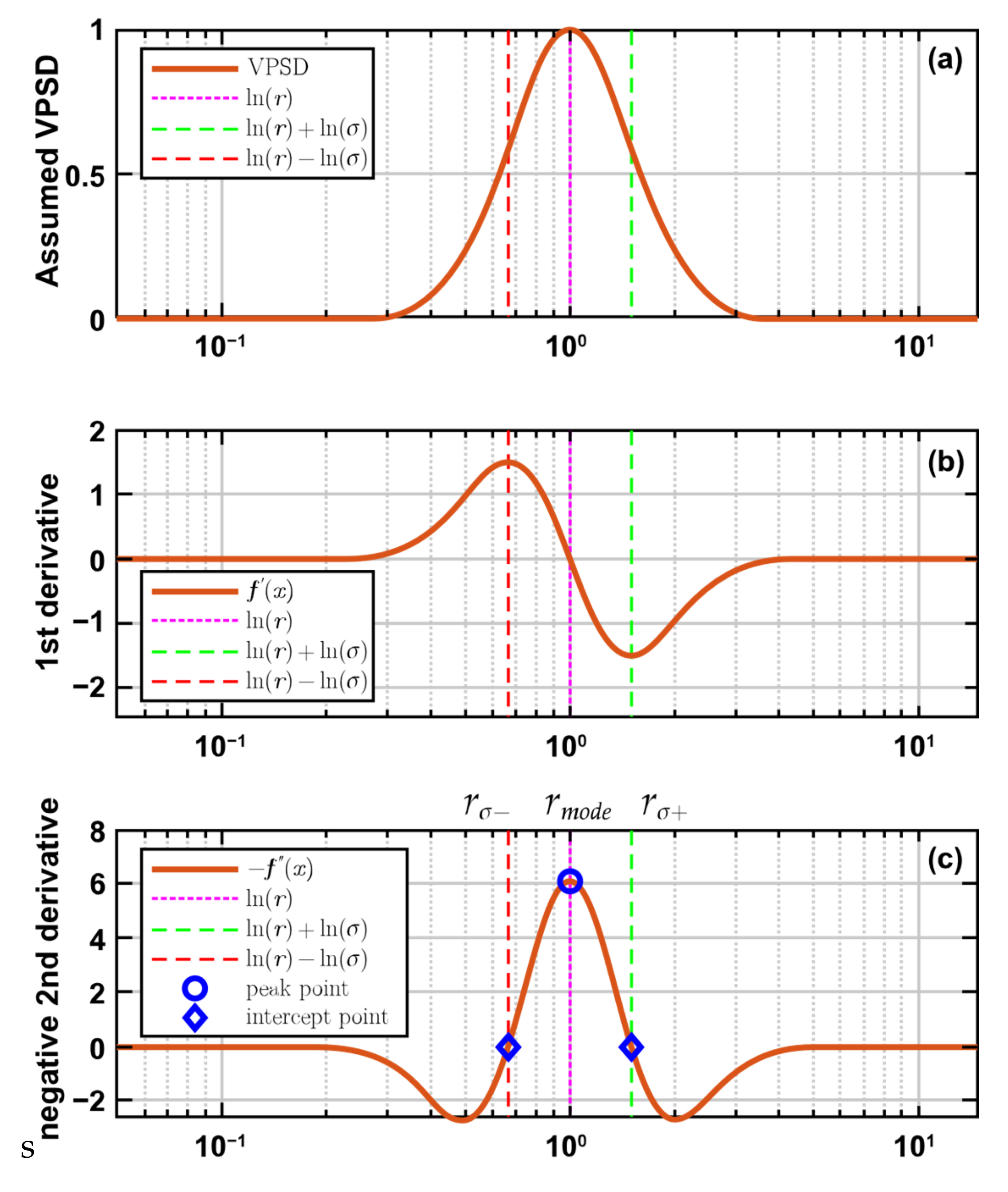
2.3. Size Distribution Mode Decomposition
3. Regional Aerosol Model
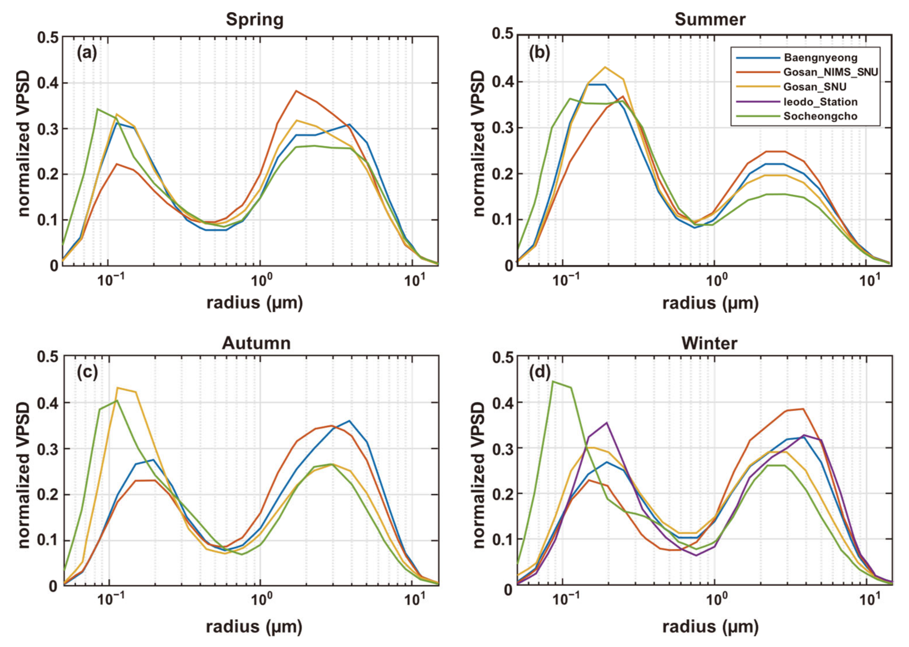
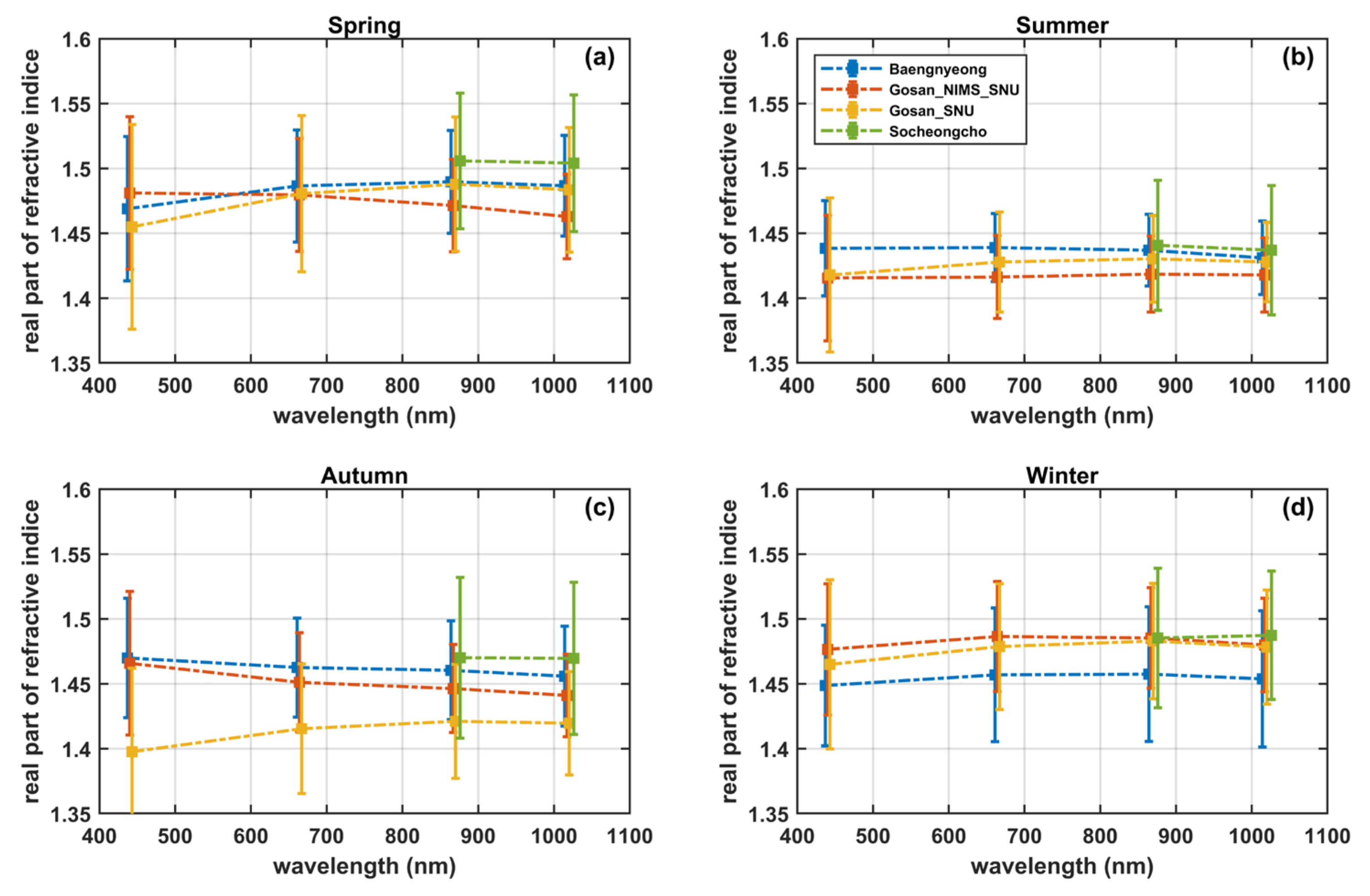
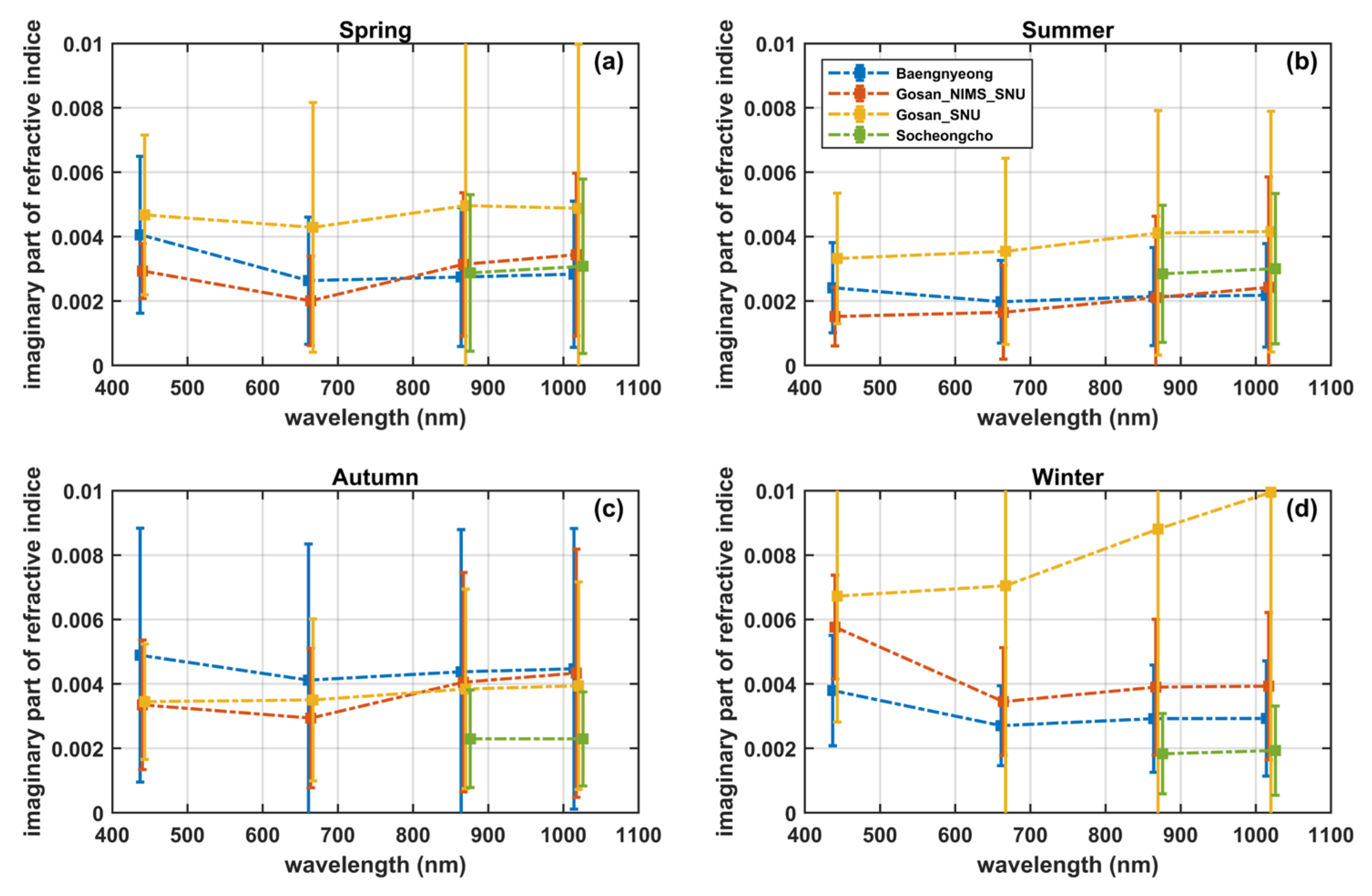
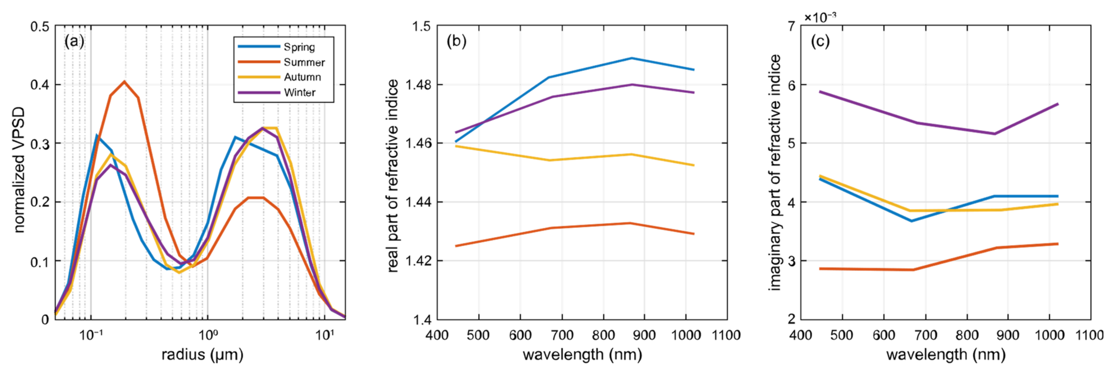
3.1. Seasonal Aerosol Model
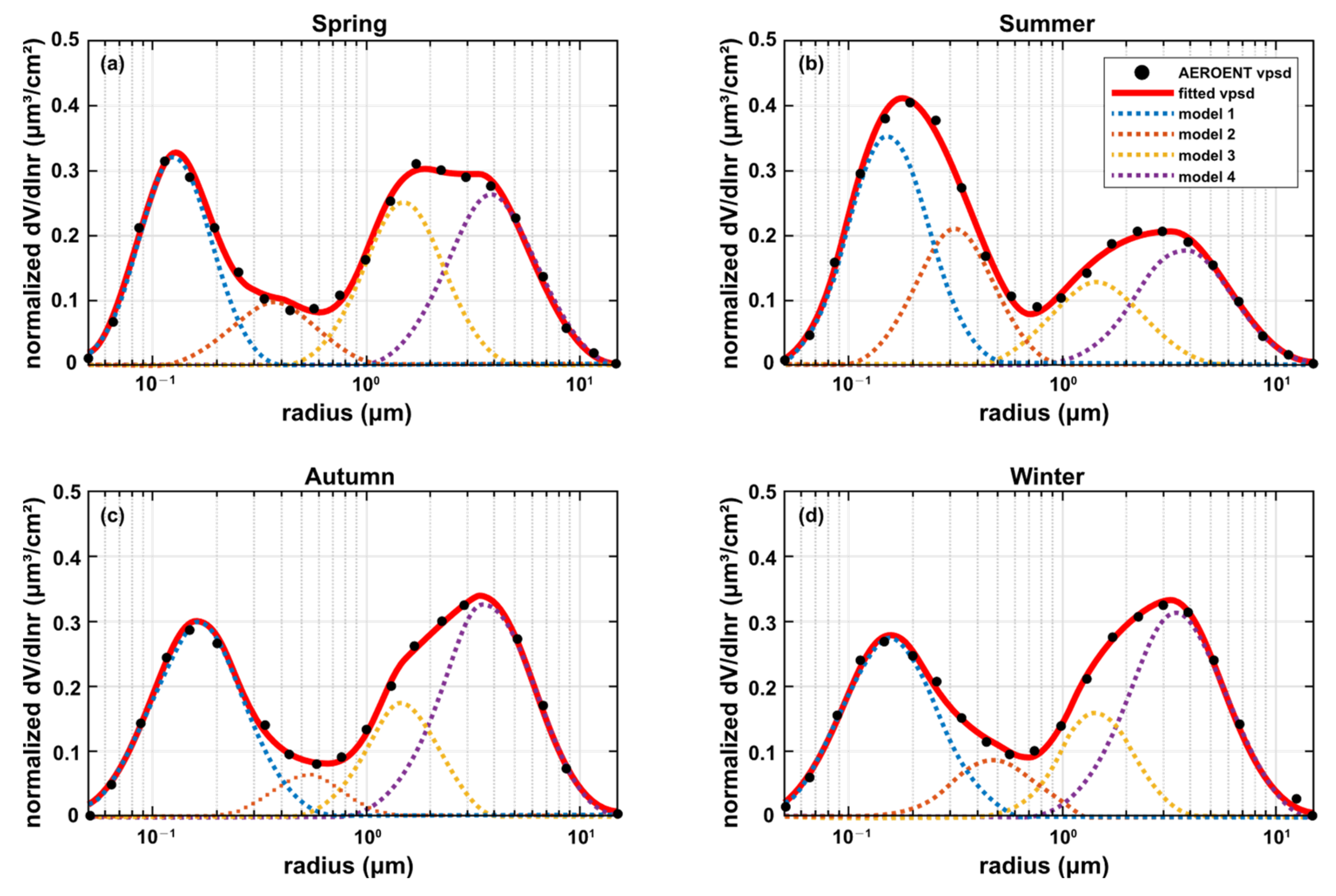
3.2. Size Distribution Mode Decomposition
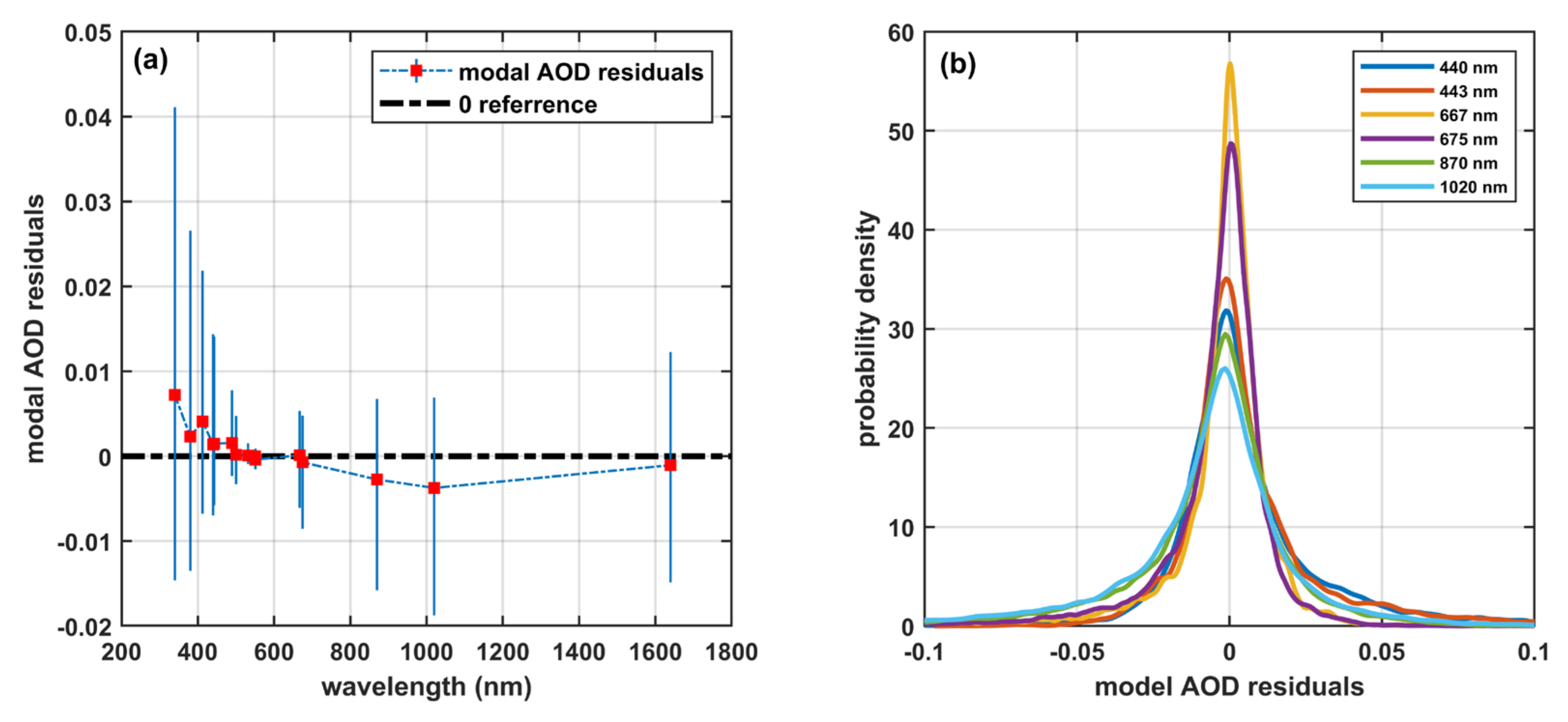
4. Evaluation
5. Conclusions
Author Contributions
Funding
Data Availability Statement
Acknowledgments
Conflicts of Interest
References
- Wang, J.; Shilling, J.E.; Liu, J.; Zelenyuk, A.; Bell, D.M.; Petters, M.D.; Thalman, R.; Mei, F.; Zaveri, R.A.; Zheng, G. Cloud droplet activation of secondary organic aerosol is mainly controlled by molecular weight, not water solubility. Atmos. Chem. Phys. 2019, 19, 941–954. [Google Scholar] [CrossRef]
- Tan, W.; He, H.; Chen, X.; Qi, W.; Liu, J.; Wang, Y.; Ling, Z.; Sun, Y.; Jin, D. Analyzing the influence of atmosphere on optical remote sensing in 400 to 2500 nm wavelength spectrum. In AOPC 2020: Optical Spectroscopy and Imaging; and Biomedical Optics; SPIE: New York, NY, USA, 2020; Volume 11566, pp. 103–108. [Google Scholar]
- Contini, D.; Lin, Y.-H.; Hänninen, O.; Viana, M. Contribution of Aerosol Sources to Health Impacts. Atmosphere 2021, 12, 730. [Google Scholar] [CrossRef]
- Liu, X.; Easter, R.C.; Ghan, S.J. Toward a minimal representation of aerosol direct and indirect effects: Model description and evaluation. Geosci. Model Dev. 2012, 5, 709–735. [Google Scholar] [CrossRef]
- Hess, M.; Koepke, P.; Schult, I. Optical Properties of Aerosols and cloud: The Software Package OPAC. Bull. Am. Meteorol. Soc. 1998, 79, 831–844. [Google Scholar] [CrossRef]
- Van Eijk, A.M.J.; Kusmierczyk-Michulec, J.T.; Piazzola, J.J. The Advanced Navy Aerosol Model (ANAM): Validation of small-particle modes. In Proceedings of the SPIE Optical Engineering + Applications, San Diego, CA, USA, 21–25 August 2011; pp. 816108–816109. [Google Scholar]
- Piazzola, J.; Bouchara, F.; de Leeuw, G.; Van Eijk, A.M.J. Development of the Mediterranean extinction code (MEDEX). Opt. Eng. 2003, 42, 912–924. [Google Scholar] [CrossRef]
- Xie, Y.S.; Li, Z.Q.; Zhang, Y.X.; Zhang, Y.; Li, D.H.; Li, K.T.; Xu, H.; Zhang, Y.; Wang, Y.Q.; Chen, X.F.; et al. Estimation of atmospheric aerosol composition from ground-based remote sensing measurements of Sun-sky radiometer. J. Geophys. Res.-Atmos. 2017, 122, 498–518. [Google Scholar] [CrossRef]
- Tombette, M.; Sportisse, B. Aerosol modeling at a regional scale: Model-to-data comparison and sensitivity analysis over Greater Paris. Atmos. Environ. 2007, 41, 6941–6950. [Google Scholar] [CrossRef]
- Zhou, P.; Wang, Y.; Liu, J.; Xu, L.; Chen, X.; Zhang, L. Difference between global and regional aerosol model classifications and associated implications for spaceborne aerosol optical depth retrieval. Atmos. Environ. 2023, 300, 119674. [Google Scholar] [CrossRef]
- Cattrall, C.; Reagan, J.; Thome, K.; Dubovik, O. Variability of aerosol and spectral lidar and backscatter and extinction ratios of key aerosol types derived from selected Aerosol Robotic Network locations. J. Geophys. Res.-Atmos. 2005, 110, 15. [Google Scholar] [CrossRef]
- Shi, Y.R.; Levy, R.C.; Yang, L.; Remer, L.A.; Mattoo, S.; Dubovik, O. A Dark Target research aerosol algorithm for MODIS observations over eastern China: Increasing coverage while maintaining accuracy at high aerosol loading. Atmos. Meas. Tech. 2021, 14, 3449–3468. [Google Scholar] [CrossRef]
- Park, J.; Dall’Osto, M.; Park, K.; Gim, Y.; Kang, H.J.; Jang, E.; Park, K.-T.; Park, M.; Yum, S.S.; Jung, J.; et al. Shipborne observations reveal contrasting Arctic marine, Arctic terrestrial and Pacific marine aerosol properties. Atmos. Chem. Phys. 2020, 20, 5573–5590. [Google Scholar] [CrossRef]
- Fan, Y.; Sun, X.; Huang, H.; Ti, R.; Liu, X. The primary aerosol models and distribution characteristics over China based on the AERONET data. J. Quant. Spectrosc. Radiat. Transf. 2021, 275, 107888. [Google Scholar] [CrossRef]
- Pani, S.K.; Huang, H.-Y.; Wang, S.-H.; Holben, B.N.; Lin, N.-H. Long-term observation of columnar aerosol optical properties over the remote South China Sea. Sci. Total Environ. 2023, 905, 167113. [Google Scholar] [CrossRef]
- Lim, Y.-K.; Kim, J.; Lee, H.C.; Lee, S.-S.; Cha, J.-W.; Ryoo, S.B. Aerosol Physical Characteristics over the Yellow Sea During the KORUS-AQ Field Campaign: Observations and Air Quality Model Simulations. Asia-Pac. J. Atmos. Sci. 2019, 55, 629–640. [Google Scholar] [CrossRef]
- Pan, Y.; Cui, S.; Rao, R. A Model for Predicting Coastal Aerosol Size Distributions in Chinese Seas. Earth Space Sci. 2020, 7, 11. [Google Scholar] [CrossRef]
- Dubovik, O.; King, M.D. A flexible inversion algorithm for retrieval of aerosol optical properties from Sun and sky radiance measurements. J. Geophys. Res.-Atmos. 2000, 105, 20673–20696. [Google Scholar] [CrossRef]
- Che, Y.; Yu, B.; Parsons, K.; Desha, C.; Ramezani, M. Evaluation and comparison of MERRA-2 AOD and DAOD with MODIS DeepBlue and AERONET data in Australia. Atmos. Environ. 2022, 277, 119054. [Google Scholar] [CrossRef]
- Sinyuk, A.; Holben, B.N.; Eck, T.F.; Giles, D.M.; Slutsker, I.; Korkin, S.; Schafer, J.S.; Smirnov, A.; Sorokin, M.; Lyapustin, A. The AERONET Version 3 aerosol retrieval algorithm, associated uncertainties and comparisons to Version 2. Atmos. Meas. Tech. 2020, 13, 3375–3411. [Google Scholar] [CrossRef]
- Sayer, A.M.; Smirnov, A.; Hsu, N.C.; Holben, B.N. A pure marine aerosol model, for use in remote sensing applications. J. Geophys. Res.-Atmos. 2012, 117, 25. [Google Scholar] [CrossRef]
- Holben, B.N.; Eck, T.F.; Slutsker, I.; Tanré, D.; Buis, J.P.; Setzer, A.; Vermote, E.; Reagan, J.A.; Kaufman, Y.J.; Nakajima, T.; et al. AERONET—A Federated Instrument Network and Data Archive for Aerosol Characterization. Remote Sens. Environ. 1998, 66, 1–16. [Google Scholar] [CrossRef]
- Kim, J.H.; Yum, S.S.; Lee, Y.G.; Choi, B.C. Ship measurements of submicron aerosol size distributions over the Yellow Sea and the East China Sea. Atmos. Res. 2009, 93, 700–714. [Google Scholar] [CrossRef]
- Cuesta, J.; Flamant, P.H.; Flamant, C. Synergetic technique combining elastic backscatter lidar data and sunphotometer AERONET inversion for retrieval by layer of aerosol optical and microphysical properties. Appl. Opt. 2008, 47, 4598–4611. [Google Scholar] [CrossRef] [PubMed]
- Taylor, M.; Kazadzis, S.; Gerasopoulos, E. Multi-modal analysis of aerosol robotic network size distributions for remote sensing applications: Dominant aerosol type cases. Atmos. Meas. Tech. 2014, 7, 839–858. [Google Scholar] [CrossRef]
- Hussein, T.; Dal Maso, M.; Petäjä, T.; Koponen, I.K.; Paatero, P.; Aalto, P.P.; Hämeri, K.; Kulmala, M. Evaluation of an automatic algorithm for fitting the particle number size distributions. Boreal Environ. Res. 2005, 10, 337. [Google Scholar]
- He, H.L.; Song, J.B.; Bai, Y.F.; Xu, Y.; Wang, J.J.; Bi, F. Climate and extrema of ocean waves in the East China Sea. Sci. China-Earth Sci. 2018, 61, 980–994. [Google Scholar] [CrossRef]
- Ganguly, D.; Raman, M. Estimating the Wind Dependency of Aerosol Optical Depth at Remote Oceanic Regions. Mar. Geod. 2023, 46, 359–375. [Google Scholar] [CrossRef]
- Liu, S.; Liu, C.-C.; Froyd, K.D.; Schill, G.P.; Murphy, D.M.; Bui, T.P.; Dean-Day, J.M.; Weinzierl, B.; Dollner, M.; Diskin, G.S.; et al. Sea spray aerosol concentration modulated by sea surface temperature. Proc. Natl. Acad. Sci. USA 2021, 118, 6. [Google Scholar] [CrossRef]
- Liu, N.; Luo, T.; Han, Y.; Yang, K.; Zhang, K.; Wu, Y.; Weng, N.; Li, X. Analysis of the atmospheric visibility influencing factors under sea–land breeze circulation. Opt. Express 2022, 30, 7356. [Google Scholar] [CrossRef]
- Shen, X.; Bilal, M.; Qiu, Z.; Sun, D.; Wang, S.; Zhu, W. Long-term spatiotemporal variations of aerosol optical depth over Yellow and Bohai Sea. Environ. Sci. Pollut. Res. 2019, 26, 7969–7979. [Google Scholar] [CrossRef] [PubMed]
- Park, S.; Yu, G.-H. Absorption properties and size distribution of aerosol particles during the fall season at an urban site of Gwangju, Korea. Environ. Eng. Res. 2019, 24, 159–172. [Google Scholar] [CrossRef]
- Wang, F.; Feng, T.; Guo, Z.; Li, Y.; Lin, T.; Rose, N.L. Sources and dry deposition of carbonaceous aerosols over the coastal East China Sea: Implications for anthropogenic pollutant pathways and deposition. Environ. Pollut. 2019, 245, 771–779. [Google Scholar] [CrossRef] [PubMed]
- Guan, X.; Wang, M.; Du, T.; Tian, P.; Zhang, N.; Shi, J.; Chang, Y.; Zhang, L.; Zhang, M.; Song, X.; et al. Wintertime aerosol optical properties in Lanzhou, Northwest China: Emphasis on the rapid increase of aerosol absorption under high particulate pollution. Atmos. Environ. 2021, 246, 118081. [Google Scholar] [CrossRef]
- Park, S.; Kim, S.-W.; Lin, N.-H.; Pani, S.K.; Sheridan, P.J.; Andrews, E. Variability of Aerosol Optical Properties Observed at a Polluted Marine (Gosan, Korea) and a High-altitude Mountain (Lulin, Taiwan) Site in the Asian Continental Outflow. Aerosol Air Qual. Res. 2019, 19, 1272–1283. [Google Scholar] [CrossRef]
- Schuster, G.L.; Dubovik, O.; Arola, A. Remote sensing of soot carbon—Part 1: Distinguishing different absorbing aerosol species. Atmos. Chem. Phys. 2016, 16, 1565–1585. [Google Scholar] [CrossRef]
- Kai, Z.; Huiwang, G. The characteristics of Asian-dust storms during 2000-2002: From the source to the sea. Atmos. Environ. 2007, 41, 9136–9145. [Google Scholar] [CrossRef]
- Li, Z.; Zhang, Y.; Xu, H.; Li, K.; Dubovik, O.; Goloub, P. The Fundamental Aerosol Models Over China Region: A Cluster Analysis of the Ground-Based Remote Sensing Measurements of Total Columnar Atmosphere. Geophys. Res. Lett. 2019, 46, 4924–4932. [Google Scholar] [CrossRef]
- Lewis, E.R.; Schwartz, S.E. Sea Salt Aerosol Production: Mechanisms, Methods, Measurements, and Models; American Geophysical Union: Washington, DC, USA, 2004; Volume 152. [Google Scholar]
- Dubovik, O.; Smirnov, A.; Holben, B.N.; King, M.D.; Kaufman, Y.J.; Eck, T.F.; Slutsker, I. Accuracy assessments of aerosol optical properties retrieved from Aerosol Robotic Network (AERONET) Sun and sky radiance measurements. J. Geophys. Res. Atmos. 2000, 105, 9791–9806. [Google Scholar] [CrossRef]


| Site Name | Time Period (Start/Stop) | AOD Counts | AOD Season Counts * | VPSD Counts | VPSD Season Counts * |
|---|---|---|---|---|---|
| Baengnyeong | 15 July 2010/30 January 2023 | 30,985 | 12,138/6994/7758/4095 | 1169 | 469/169/466/65 |
| Gosan_NIMS_SNU | 22 June 2020/1 January 2022 | 14,053 | 3761/2168/5496/2628 | 676 | 160/47/300/169 |
| Gosan_SNU | 3 April 2001/13 September 2016 | 32,659 | 16,612/9611/3740/2696 | 1371 | 820/245/154/152 |
| Ieodo_Station | 30 November 2013/18 August 2019 | 4413 | 2120/568/624/1101 | 2 | 0/0/0/2 |
| Socheongcho | 12 October 2015/5 November 2021 | 24,711 | 8644/5104/7083/3880 | 296 | 133/39/72/52 |
| Season | Mode 1 | Mode 2 | Mode 3 | Mode 4 | ||||||||
|---|---|---|---|---|---|---|---|---|---|---|---|---|
| Spring | 0.31 | 1.47 | 0.13 | 0.11 | 1.59 | 0.37 | 0.27 | 1.53 | 1.50 | 0.31 | 1.60 | 3.83 |
| Summer | 0.39 | 1.54 | 0.15 | 0.22 | 1.51 | 0.31 | 0.16 | 1.65 | 1.44 | 0.24 | 1.69 | 3.72 |
| Autumn | 0.37 | 1.64 | 0.16 | 0.06 | 1.44 | 0.53 | 0.17 | 1.47 | 1.47 | 0.41 | 1.65 | 3.69 |
| Winter | 0.35 | 1.65 | 0.15 | 0.09 | 1.53 | 0.46 | 0.16 | 1.48 | 1.43 | 0.41 | 1.67 | 3.44 |
Disclaimer/Publisher’s Note: The statements, opinions and data contained in all publications are solely those of the individual author(s) and contributor(s) and not of MDPI and/or the editor(s). MDPI and/or the editor(s) disclaim responsibility for any injury to people or property resulting from any ideas, methods, instructions or products referred to in the content. |
© 2024 by the authors. Licensee MDPI, Basel, Switzerland. This article is an open access article distributed under the terms and conditions of the Creative Commons Attribution (CC BY) license (https://creativecommons.org/licenses/by/4.0/).
Share and Cite
Chen, S.; Dai, C.; Liu, N.; Lian, W.; Zhang, Y.; Wu, F.; Zhang, C.; Cui, S.; Wei, H. A Regional Aerosol Model for the Oceanic Area around Eastern China Based on Aerosol Robotic Network (AERONET). Remote Sens. 2024, 16, 1106. https://doi.org/10.3390/rs16061106
Chen S, Dai C, Liu N, Lian W, Zhang Y, Wu F, Zhang C, Cui S, Wei H. A Regional Aerosol Model for the Oceanic Area around Eastern China Based on Aerosol Robotic Network (AERONET). Remote Sensing. 2024; 16(6):1106. https://doi.org/10.3390/rs16061106
Chicago/Turabian StyleChen, Shunping, Congming Dai, Nana Liu, Wentao Lian, Yuxuan Zhang, Fan Wu, Cong Zhang, Shengcheng Cui, and Heli Wei. 2024. "A Regional Aerosol Model for the Oceanic Area around Eastern China Based on Aerosol Robotic Network (AERONET)" Remote Sensing 16, no. 6: 1106. https://doi.org/10.3390/rs16061106