Assessment of Sea-Ice Classification Capabilities during Melting Period Using Airborne Multi-Frequency PolSAR Data

Abstract

Sea-ice mapping using Synthetic Aperture Radar (SAR) in the melt season poses challenges, primarily due to meltwater complicating the distinguishability of sea-ice types. In response to this issue, this study introduces a novel method for classifying sea ice during the Bohai Sea’s melting period. The method categorizes sea ice into five types: open water (OW), gray ice (Gi), melting gray ice (GiW), gray–white Ice (Gw), and melting gray–white Ice (GwW). To achieve this classification, 51 polarimetric features are extracted from L-, S-, and C-band PolSAR data using various polarization decomposition methods. This study assesses the separability of these features among different combinations of sea-ice type by calculating the Euclidean distance (ED). The Support Vector Machine (SVM) classifier, when employed with single-frequency polarimetric feature sets, achieves the highest accuracy for OW and Gi in the C-band, GiW in the S-band, and Gw and GwW in the L-band. Remarkably, the C-band features exhibit the overall highest accuracy when compared to the L-band and S-band. Furthermore, employing a multi-dimensional polarimetric feature set significantly improves classification accuracy to 94.55%, representing a substantial enhancement of 9% to 22% compared to single-frequency classification. Benefiting from the performance advantages of Random Forest (RF) classifiers in handling large datasets, RF classifiers achieve the highest classification accuracy of 95.84%. The optimal multi-dimensional feature composition includes the following: L-band: SE, SE_I, $\overline{\mathsf{\alpha }}$, Span; S-band: SE_I, SE, Span, P_V-Freeman, λ₁, λ₂; C-band: SE, SE_I, Span, λ₃, P_V-Freeman. The results of this study provide a reliable new method for future sea-ice monitoring during the melting season.

1. Introduction

Sea ice, as a vital component of the oceanic system, exerts a substantial influence on the ocean’s physical characteristics, including temperature, salinity, and density. This, in turn, has a profound impact on ocean circulation and the broader climate system [1]. Furthermore, sea ice can have varying degrees of detrimental effects on multiple industries, including shipping, offshore oil and gas exploration, as well as marine fisheries [2]. Therefore, it is of paramount importance to conduct timely and precise monitoring of sea ice in order to preempt and alleviate the losses resulting from sea-ice disasters. The classification of sea ice, a pivotal element in the realm of sea-ice research, forms the cornerstone of sea-ice monitoring efforts. Diverse information pertaining to sea ice, including data on sea-ice concentration, extent, and thickness, can be derived from the outcomes of sea-ice classification [3,4,5].

Many current sea-ice studies focus on the freezing period, but research on sea ice during the melting season is equally significant. The melting season is a dynamic and crucial phase in the sea-ice system, marking the melting and degradation of sea ice. During the melting process, sea ice absorbs a substantial amount of heat, playing a role in regulating the temperature of the surrounding water and the atmosphere, helping to prevent rapid temperature increases. Additionally, sea-ice melting alters seawater salinity and density, affecting the surface ocean circulation. Melting ice also results in a reduction in sea-ice coverage, resulting in an impact on the reflection of solar radiation and heat absorption in the ocean. Therefore, the melting season has profound implications for the climate and marine ecosystems in regions with sea ice [6]. During the melting period, the atmosphere contains a higher water vapor content, which can result in the formation of clouds and fog. Traditional visible light and infrared remote sensing data perform poorly in such conditions. Microwave remote sensing, with its all-weather and all-day advantages, has become a practical tool for monitoring sea ice [7]. Microwave remote sensing data provide essential support for better understanding and addressing the impacts of climate change.

Starting from June 1978 with the launch of the first spaceborne Synthetic Aperture Radar (SAR) satellite, Seasat, by the United States, humanity achieved around-the-clock and all-weather monitoring of sea ice for the first time. With the subsequent launch of other SAR systems and their extensive application in sea-ice monitoring, many countries and regions have established operational sea-ice monitoring capabilities [8].

SAR has demonstrated excellent performance in various fields and has garnered significant attention from many countries, becoming a highly competitive and rapidly evolving technological field. Starting from 1990, SAR systems have evolved from the initial L-band HH single-polarization system to multi-frequency systems (L, C, X) with four polarization modes (HH, HV, VV, VH). Multi-dimensional SAR systems have broken free from the constraints of single-polarization or dual-polarization SAR data. Compared to single- or dual-polarization SAR, polarimetric Synthetic Aperture Radar (PolSAR) provides more information about sea ice, including phase information and higher spatial resolution, enhancing the potential of SAR in environmental monitoring [9,10,11].

SAR belongs to the category of imaging sensors, and in the context of sea-ice classification research based on SAR data, researchers can use SAR images for classification and identification. For instance, R. De Abreu [12] discussed the differences in open water, new ice, and gray ice on different polarization images and performed classification. Kwon et al. [13] proposed a total variation optimal segmentation method for sea-ice SAR images, reducing image processing time while improving segmentation accuracy. Johannessen et al. [14], based on texture features in sea-ice SAR images, utilized neural network algorithms and Bayesian discrimination for sea-ice image type recognition. Wang et al. [15] introduced a segmentation and classification method for sea-ice SAR images based on Markov random field theory and ice condition maps, which effectively suppressed the impact of speckle noise and enhanced image segmentation and classification accuracy. Liu et al. [16], using a second-order classification method based on covariance, classified sea-ice SAR images from the RADARSAT-2 satellite over Liaodong Bay.

Furthermore, a multitude of research scholars have proposed various polarization parameters for sea-ice classification [17,18,19], and the reliability of these parameters has been widely recognized and applied within the academic community. For instance, Zhang et al. [20] achieved accurate classification of Bohai Sea ice using H/α decomposition, Freeman decomposition, and polarization basis transformation features based on C-band RADARSAT-2 SAR data. Scheuchl et al. [21] utilized full-polarization data in the C-band to extract polarization ratios and other polarization information for sea-ice type recognition in SAR images. Dabboor et al. [22] developed a new SAR polarization feature for sea-ice classification using the coherence matrix of fully polarized SAR images. Zhang et al. [23] describes a three-component scattering model to decompose PolSAR data of sea ice. The model is validated using C-band RADARSAT-2 quad-polarization data acquired over sea ice in the Bohai Sea. Many researchers have also devised various deep learning methods suitable for sea-ice classification [24,25], and these methods have demonstrated effective classification results in both polar regions.

Many of the aforementioned works have, to some extent, utilized SAR’s polarization information and explored the effects of different features on sea-ice classification. However, these works have been based on single-frequency SAR data and lack an in-depth study of the connection between the electromagnetic scattering characteristics of sea-ice targets and electromagnetic wave frequencies. In order to better understand the electromagnetic scattering characteristics of sea ice at different frequencies and to improve the accuracy and reliability of sea-ice classification, Rignot et al. [26] conducted experiments on sea-ice classification using multi-frequency SAR data from the airborne AIRSAR system in the Beaufort Sea. The experimental results demonstrated that using multi-frequency polarimetric feature data can significantly improve sea-ice classification accuracy, with classification accuracy increasing by 14% to 20% compared to single-frequency, single-polarization data. Xie et al. [27] analyzed and discussed the advantages and limitations of combining dual-band SAR polarimetric features for SAR sea-ice classification and recognition, using C- and L-band fully polarized sea-ice SAR data acquired by the SIR-C SAR system in the Weddell Sea, Antarctica. These studies collectively indicate that utilizing multi-dimensional SAR data for sea-ice classification is an effective means to enhance SAR sea-ice type recognition capabilities.

Many of the existing sea-ice classification studies mentioned above are primarily based on the freezing period. With variations in sea-ice age, ice thickness, SAR system wavelength, and incidence angle, the scattering mechanisms of sea ice also differ [28]. Furthermore, during the melting period, the presence of surface meltwater on sea ice absorbs electromagnetic waves, making the scattering characteristics on the sea-ice surface complex and challenging to differentiate. This complexity leads to sea-ice classification methods and features that are effective during the freezing period often yielding unsatisfactory results during the melting period [21].

Therefore, two main factors hinder the accurate classification of sea ice during the melting period. Firstly, there is already a wealth of polarization features available for sea-ice classification, but the classification capabilities of multi-frequency polarization features for sea ice during the melting period have not been fully explored. Secondly, although many classifiers have been applied to sea-ice classification, the impact of different combinations of classifiers and feature sets on sea-ice classification results remains uncertain.

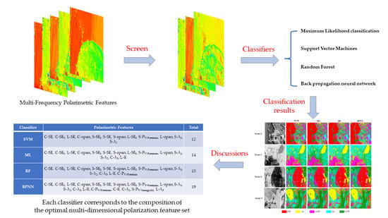
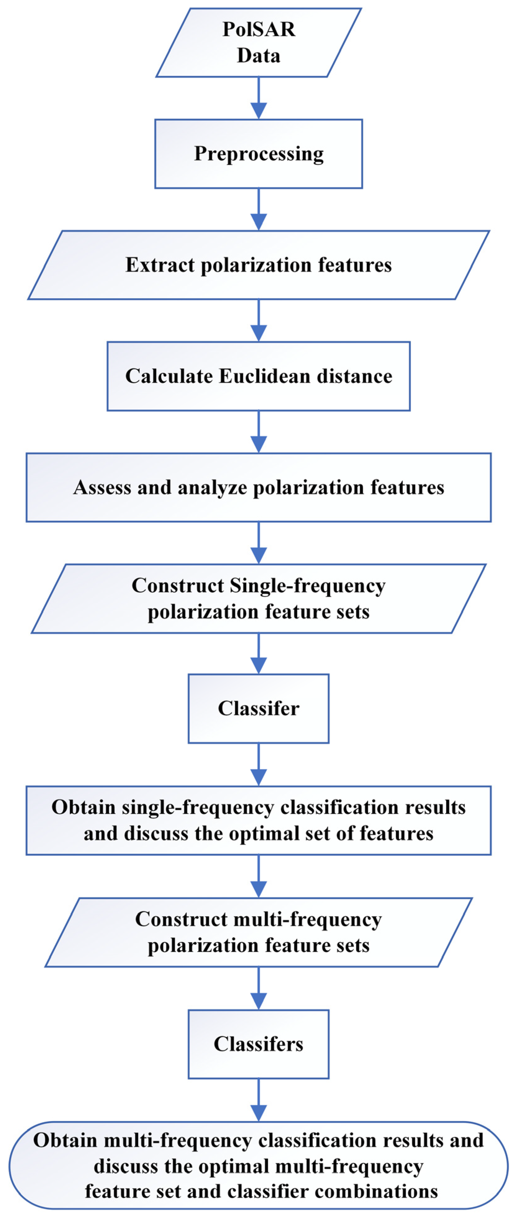
To address the scientific questions mentioned above, this study contributes in the following three ways: First, we conducted, for the first time, an experiment to acquire multi-frequency, fully polarimetric PolSAR sea-ice data during the melting season in the Bohai Sea region. The experimental data include three frequency bands: L, S, and C. Second, we assessed the separability of polarimetric features for various sea-ice type combinations and analyzed the distinctions and connections among polarimetric features in different frequency bands. Third, we introduced a sea-ice classification method for the melting season based on multi-frequency and multi-polarization PolSAR polarimetric feature selection. We analyzed and discussed the impact of classifier–feature set combinations on classification results.

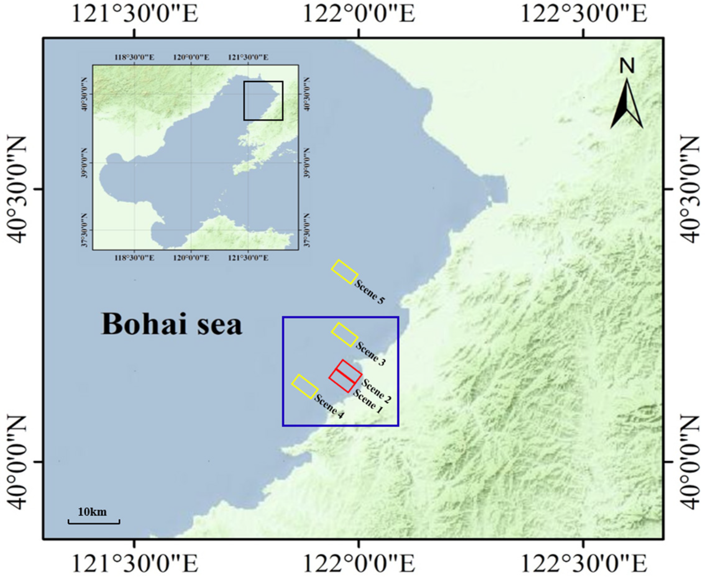
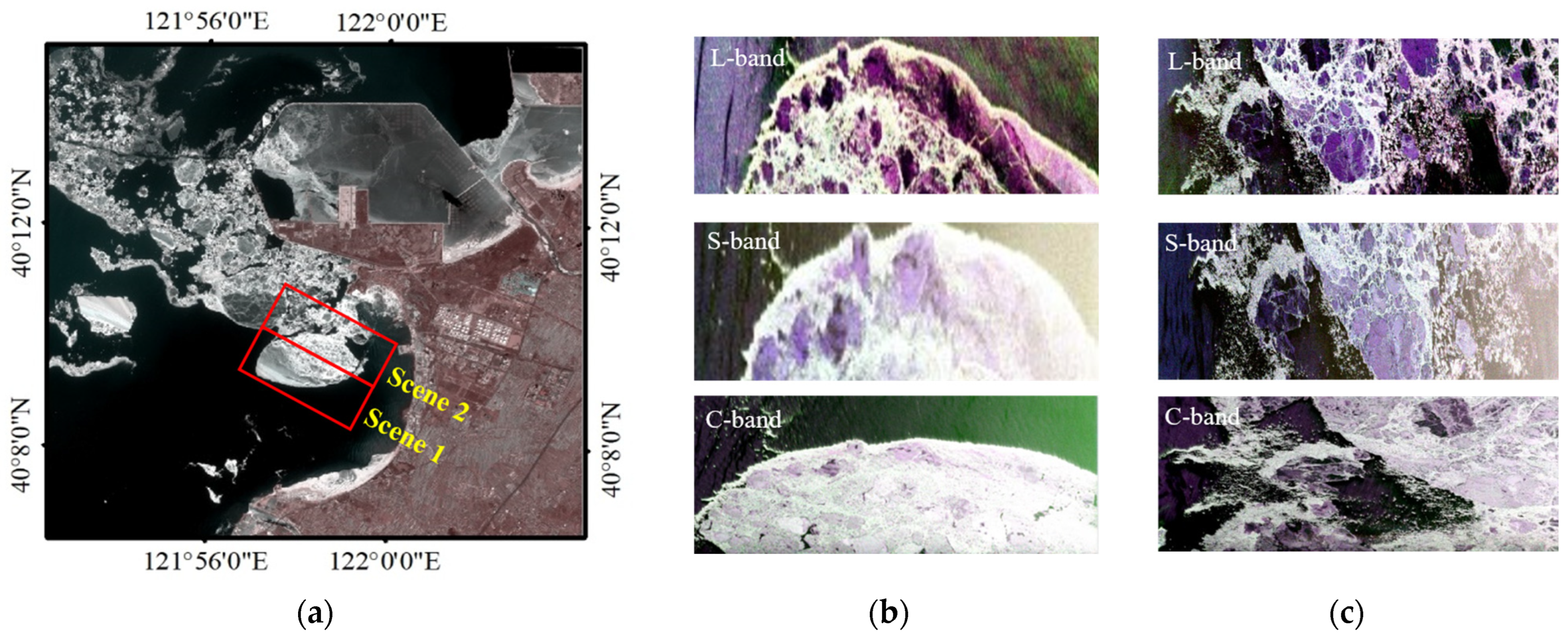
The study is organized as follows: In Section 2, the data used in the study are introduced, including airborne multi-frequency PolSAR data, Sentinel-2 data, and a description of the process for interpreting sea-ice types during the melting period. Section 3 summarizes the 51 polarimetric features used for sea-ice classification, explains how the best sea-ice classification parameters are chosen using Euclidean distance, and provides detailed information on the parameters of the selected classifiers. In Section 4, the separability strength of polarimetric features in different sea-ice type combinations in each band is evaluated, and the reasons for these differences are analyzed. Section 5 describes the classification results obtained with different combinations of classifiers and features. Finally, Section 6 concludes the study and provides a discussion of the findings.

2. Study Area and Data

2.1. Study Area

The research area for this study is located in Liaodong Bay, situated within the Bohai Sea region of China, as illustrated in Figure 1. The Bohai Sea is not only home to numerous crucial ports but also serves as a vital hub for China’s maritime trade. Furthermore, this region is rich in resources, encompassing petroleum, natural gas, and fisheries, making it strategically significant for China’s national defense and security. The Bohai Sea occupies a pivotal geographical and strategic position in China’s economic development and international interactions [2]. It is worth noting that sea ice in the Bohai Sea is of the annual type, forming during the winter and persisting until early spring of the following year.

This study utilizes two different types of remote sensing data: multi-frequency PolSAR data and Sentinel-2 optical data, with their respective coverage areas displayed in Figure 1. The PolSAR data used in this study were collected by our research team near Bayuquan in Liaodong Bay, Bohai Sea, on 27–28 February 2022, using remote sensing aircraft. The geographic coordinates covered by the data range from 40°8′N to 40°22′N and from 121°57′E to 122°10′E. Prior to the experimental survey, the local maximum temperatures had remained above 0 °C for three consecutive days, with a maximum temperature of 6 °C on the day of the experiment and 10 °C on the following day. This temperature trend indicates that the sea ice in the acquired multi-dimensional SAR data was in a melting phase, which is a crucial factor in our research focus.

The presence of sediment in the Bohai Sea may affect sea-ice classification. However, the study area in this paper is located in the Liaodong Bay, with fewer old river mouths and much lower suspended sediment content compared to Laizhou Bay, which serves as the estuary of the Yellow River. The impact of suspended sediment on sea-ice classification is more pronounced in the Laizhou Bay region, but it can be considered negligible for the experimental area in this study.

2.2. Multi-Dimensional PolSAR Data

The SAR data used in this experiment were acquired by a Modern Ark 60 remote sensing aircraft equipped with a multi-dimensional SAR system. The remote sensing aircraft is equipped with various payloads, including three-line array cameras, area array cameras, and a multi-dimensional SAR system. The multi-dimensional SAR system is a set of multi-frequency, fully polarimetric SAR systems that use a distributed phased array antenna with electronically steerable radar beams. It is capable of acquiring high-resolution backscatter data from the ground.

This study utilized data from three subsystems, L-band, S-band, and C-band, of a multi-dimensional SAR system, comprising a total of five scenes. Scene 1 and Scene 2 were collected on the 27th, while Scene 3, Scene 4, and Scene 5 were collected on the 28th. All these scenes encompass all types of sea ice discussed during the melting period. Detailed information about the SAR data is provided in

Table 1. Multi-dimensional SAR parameters and basic information of data.

Band	Resolution (m)	Polarization Mode	Scene	Incidence Angle (°)	Acquisition Start Time UTC
L	1.0	HH/HV/VH/VV	Scene 1	31.89	2022-02-27 06:22:54
			Scene 2	31.89	2022-02-27 06:23:23
			Scene 3	31.86	2022-02-28 03:13:55
			Scene 4	31.86	2022-02-28 03:17:25
			Scene 5	31.86	2022-02-28 03:27:30
S	1.0	HH/HV/VH/VV	Scene 1	33.51	2022-02-27 06:22:54
			Scene 2	33.51	2022-02-27 06:23:23
			Scene 3	33.48	2022-02-28 03:13:55
			Scene 4	33.48	2022-02-28 03:17:25
			Scene 5	33.48	2022-02-28 03:27:30
C	0.5	HH/HV/VH/VV	Scene 1	33.51	2022-02-27 06:22:54
			Scene 2	33.51	2022-02-27 06:23:23
			Scene 3	33.48	2022-02-28 03:13:55
			Scene 4	33.48	2022-02-28 03:17:25
			Scene 5	33.48	2022-02-28 03:27:30

.

2.3. Sentinel-2 Data

Sentinel-2 is a high-resolution multispectral imaging satellite that carries a multispectral imager capable of covering 13 spectral bands with a spatial resolution of 10 m. It consists of two satellites, Sentinel-2A and Sentinel-2B [29]. In this study, optical data acquired by Sentinel-2B were used. The data collection began on 27 February 2022, at 02:36:39 (UTC). The data product level is L1C, which means it has undergone orthorectification and geometric correction, resulting in atmospheric apparent reflectance products. The time interval between the acquisition of Sentinel-2 optical data and the multi-dimensional SAR data is less than 4 h, which assists in visual interpretation of sea-ice types and sample selection. The following table provides detailed information on each band of the Sentinel-2B satellite.

2.4. Visual Interpretation of Sea-Ice Types

The current sea-ice naming standard for the Bohai Sea primarily focuses on sea-ice types during the freezing period and does not provide detailed classification for sea-ice types during the melting period [30]. While we did not have access to field measurements to validate the results, in this study, we utilized Sentinel-2 data with a resolution of 10 m to determine sea-ice types, enhancing the credibility of our approach. Simultaneously, we sought the expertise of multiple sea-ice research specialists to assess the sea-ice types in the experimental area, ensuring the accuracy of the sea-ice validation results. This study specifically classifies the sea ice in the experimental data into five types: open water (OW), gray ice (Gi), melting gray ice (GiW), gray–white Ice (Gw), and melting gray–white ice (GwW). This classification accounts for sea-ice types during the melting period and provides a more detailed breakdown of the sea-ice categories.

In Figure 2, the original states of the images for each band are displayed. Figure 3 shows the geographically registered images for each band, providing a visual observation of the differences in sea ice at the same location. As depicted in Figure 3, in optical imagery, OW appears relatively dark when compared to other sea-ice types. This is because seawater has a strong absorbent capacity for visible light. Gi and GiW have flat and wet surfaces, often appearing as extensive, concentrated patches or small gray ice sheets in the image. GiW, due to a higher degree of melting, appears darker than Gi. Gw is typically found around and overlapping with Gi, has a rough surface, and exhibits a stronger reflectance in visible light, making it appear brighter and gray–white in the image. Due to the presence of meltwater, GwW may appear slightly dimmer than Gw but is rougher and has a higher brightness compared to Gi.

Figure 2. (a) Sentinel-2 true-color image (R = band 4, G = band 3, B = band 2, specific band information is available in

Table 2. Detailed information for the bands of Sentinel-2B.

Band	Central Wavelength (nm)	Bandwidth (nm)	Resolution (m)
Band 1—Coastal aerosol	442.2	20	60
Band 2—Blue	492.1	65	10
Band 3—Green	559.0	35	10
Band 4—Red	664.9	30	10
Band 5—Vegetation red edge	703.8	15	20
Band 6—Vegetation red edge	739.1	15	20
Band 7—Vegetation red edge	779.7	20	20
Band 8—NIR	832.9	115	10
Band 8A—Narrow NIR	864.0	20	20
Band 9—Water vapor	943.2	20	60
Band 10-SWIR—Cirrus	1376.9	30	60
Band 11—SWIR	1610.4	90	20
Band 12—SWIR	2185.7	180	20

). The red rectangles in the image indicate the coverage area of the PolSAR data in Scene 1 and Scene 2. For each waveband, the partially overlapping regions in (b) Scene 1 and (c) Scene 2 are represented in Pauli RGB images.

Figure 2. (a) Sentinel-2 true-color image (R = band 4, G = band 3, B = band 2, specific band information is available in Table 2). The red rectangles in the image indicate the coverage area of the PolSAR data in Scene 1 and Scene 2. For each waveband, the partially overlapping regions in (b) Scene 1 and (c) Scene 2 are represented in Pauli RGB images.

We have listed the sea-ice types present in the study area in

Table 3. Table describing the morphology of sea ice in the study area in Sentinel-2 image.

Ice Class	Abbreviation	Morphological Feature Description
Open water	OW	The surface is smooth and the color is darker.
Gray ice	Gi	First-year floating ice, characterized by a flat surface, often appears gray.
Melting Gray ice	GiW	First-year floating ice with a wet, flat surface appears darker and is relatively thin.
Gray-white Ice	Gw	Deformed first-year floating ice has a rougher texture and appears gray–white.
Melting Gray-white Ice	GwW	Rough, gray–white first-year floating ice has a surface with a coarse texture.

and provided descriptions of the natural morphology of sea-ice as observed in optical images.

In the L-band imagery, some GiW exhibits relatively low brightness, which is close to the brightness of OW. This is because GiW has the lowest ice thickness and a wet surface, resulting in similar backscattering coefficients between GiW and OW. It is also evident that Gi is often accompanied by Gw, and the two exhibit a noticeable difference in brightness, with Gi having a distinct and visible outline. Similar to optical imagery, the highest brightness is observed in Gw, but it can be challenging to distinguish it from GwW with the naked eye. In the S-band imagery, OW has the lowest brightness, making it relatively easy to distinguish from sea ice. Compared to the L-band, the brightness difference between Gi and Gw in the S-band is less pronounced, and both GiW and Gw exhibit bright characteristics with minimal brightness difference. In the C-band imagery, the brightness contrast between seawater and sea ice is most pronounced among the three frequency bands. However, sea-ice types have similar backscattering coefficients in the C-band, making it challenging to distinguish the brightness differences between them visually.

3. Methodology

In this study, we performed the following processing steps on the used PolSAR data: first, we applied the Refined Lee Filtering method to reduce the impact of noise on SAR data. Second, based on various polarization decomposition methods, we extracted 51 polarization features from each band. Third, to evaluate the discriminative power of these polarization features for different sea-ice combinations, we calculated the Euclidean distance of polarization features in different sea-ice combinations. Fourth, we constructed feature sets and used the recursive feature elimination method to input the feature sets into different classifiers. Finally, based on the classification results, we discussed and obtained the optimal single-frequency and multi-frequency polarization feature sets suitable for sea-ice classification during the melting period. The following Figure 4 shows the flowchart of sea-ice classification during the melting period based on multi-frequency PolSAR data.

3.1. PolSAR Data Preprocessing and Polarimetric Feature Extraction

SAR data can be affected by various types of noise during collection and processing, such as thermal noise and scattering noise. These noises can degrade the quality and details of the images, making it difficult to distinguish the edges and fine details of sea ice. First, the scattering matrix and coherence matrix are extracted from the SAR data in single-look complex (SLC) format. Subsequently, the data undergo preprocessing using the Refined Lee Filtering method with a selected window size of 7 × 7 [31]. Secondly, based on H/A/$\overline{\alpha }$ decomposition [17], Freeman–Durden decomposition [18], and Yamaguchi four-component decomposition [19], we obtained a total of 51 polarization features, and the feature information is listed in

Table 4. Polarimetric features in this study.

Polarization Decomposition Method	Symbol	Name
H/A/$\overline{\alpha }$ decomposition	λ1, λ2, λ3	Eigenvalue
	P1, P2, P3	Eigenvalue probability
	H	Entropy
	A	Anisotropy
	A12	Anisotropy12
	A (Lueneburg)	Lueneburg anisotropy
	SERD	Single-bounce eigenvalues relative difference
	DERD	Double-bounce eigenvalues relative difference
	SE	Shannon entropy
	SEP	Polarimetric component of Shannon entropy
	SEI	Intensity component of Shannon entropy
	PF	Polarization fraction
	PA	Shannon entropy
	RVI	Radar vegetation index
	PH	Pedestal height
	λ	Average Target Power
	$\overline{\alpha }$	Alpha approximation
	α1, α2, α3	Internal parameters of the Eigenvector
	β, β1, β2, β3	Target orientation Angle
	δ, δ1, δ2, δ3	Scattering diversity
	γ, γ1, γ2, γ3	Polarization characteristic parameter
	CCC	Consistency correlation coefficient
Freeman–Durden decomposition	PS-Freeman	Surface scattering (corresponding power)
	PD-Freeman	Double Bounce Scattering (corresponding power)
	PV-Freeman	Volume Scattering (corresponding power)
Yamaguchi four-component decomposition	PS-Yamaguchi	Surface scattering (corresponding power)
	PD-Yamaguchi	Double-Bounce Scattering (corresponding power)
	PV-Yamaguchi	Volume Scattering (corresponding power)
	PH-Yamaguchi	Helix Scattering (corresponding power)
Other parameters	Span	Total power of scattering matrix
	C11, C22, C33	Components of the covariance matrix
	ρ12, ρ13, ρ23	Correlation coefficient

. Since the pixel sizes of the images in different bands are different and the SAR data have not been geographically corrected, to ensure the subsequent experiments, we needed to perform geo-referencing on the polarization feature data for the three bands. We selected the overlapping areas in the three bands as the input data for the subsequent work, and the number of rows and columns in the overlapping area was set to 3000. A total of 51 parameters are used in this study, as summarized in Table 4.

3.2. Separability Index

Selecting the appropriate polarization features is a crucial step in sea-ice classification research. If the spatial dimension of the features is too small, it may be insufficient to identify the characteristics of sea ice, making it difficult to achieve the expected classification results. Conversely, using too many parameters can lead to data redundancy, reducing classification accuracy and increasing computational costs [32]. To quantitatively compare the classification capabilities of the 51 polarization features mentioned above and select the optimal features for each wavelength band, this study employs the Euclidean distance [33] to measure the strength of separability between different sea-ice types. The definition of Euclidean distance is as follows:

$$D=\frac{\left|m_1-m_2\right|}{\sqrt{{\sigma }_1^2+{\sigma }_2^2}}$$

(1)

In this context, m and σ² represent sample mean and variance, and the Euclidean distance (ED) satisfies D > 0. The larger the value of the Euclidean distance, the stronger the separability between two types of samples, and vice versa. As indicated by the above formula, the greater the difference in means and the smaller the variance between regions, the larger the ED, and thus, the stronger the separability. In this study, we calculated the ED values for any two combinations among the five types, as follows: OW–Gi, OW–GiW, OW–Gw, OW–GwW, Gi–GiW, Gi–Gw, Gi–GwW, GiW–Gw, GiW–GwW, and Gw–GwW, making a total of 10 combinations. If the ED value of polarization features in the sea-ice type combination is less than 0.6, we consider the separability of that feature within the combination to be low. When the ED value is greater than or equal to 0.6 but less than 1.2, we consider the separability to be medium. However, if the ED value is greater than or equal to 1.2, we classify it as high separability within that combination.

In addition, we calculated the average Euclidean distance values of polarization features in the 10 combinations (Ice Type) to represent the overall separability strength of that feature for all sea-ice type combinations.

$$Ice Type=\sum _{i=10}{D}_i$$

(2)

where $D_i$ represents the ED values of polarization features in the ten combinations. When the Ice Type ≥ 1.2, we consider that this polarization feature has strong overall separability capability, meeting the requirements of sea-ice classification.

Simultaneously, we calculated the average Euclidean distance (A_ED) of all polarization features that met the classification requirements in the corresponding sea-ice type combinations within each wavelength band, to represent the separability capability of the polarization features in the corresponding sea-ice type combinations.

$$A_{ED}=\frac{\sum D_j}{N}$$

(3)

where $D_j$ is the ED of the polarization features that meet the classification criteria within the selected sea-ice type combinations in this wavelength band, and N is the number of polarization features that meet the classification criteria in this wavelength band. When A_ED ≥ 1.2, we consider that the polarization features in this wavelength band have strong separability in the corresponding sea-ice combinations.

3.3. Classifier

While many scholars have developed various deep learning-based classifiers for sea-ice classification, achieving good classification accuracy, in this study, we still selected four machine learning classifiers for sea-ice classification, including Maximum Likelihood classification (ML), Support Vector Machines (SVM), Random Forest (RF), and Back propagation neural network (BPNN) [34,35,36,37]. We chose these classifiers because deep learning classifiers generate new features for classification based on existing features, making it difficult for users to understand the working principles of the model and the role of internal features. This also makes it challenging for users to intuitively assess the advantages and disadvantages of polarization features in different wavelength bands in classification. Moreover, the primary focus of this study is to evaluate the capabilities of polarization features in sea-ice classification during the melting season. In future work, we can utilize deep learning methods in conjunction with the polarization features discussed in this study to achieve higher accuracy in classification results, but this is beyond the scope of this study. The detailed information on the classifiers selected in this study, along with the corresponding parameter settings, is as follows.

(1)

ML: It is a statistical estimation-based classification method used to estimate the parameters of a probability model and make classification decisions based on likelihood. In this study, the likelihood threshold is chosen as a single value, and the data proportion coefficient is set to 1.

(2)

SVM: It transforms the original features into a high-dimensional feature space to find the optimal separating hyperplane. In this study, the radial basis function is used as the kernel function for SVM.

(3)

RF: It generates a large number of decision trees and randomly selects training samples and features for each tree. Classification is determined by the outputs of all individual classification trees, making it robust to noise. In this study, 100 classification trees are planted, and the square root method is used to determine the number of features.

(4)

BPNN: It is a highly flexible model capable of adapting to various types of data and complex relationships. In this study, the activation function is chosen as logistic, the training contribution threshold is set to 0.9, the weight adjustment speed is 0.2, the number of hidden layers is 1, the number of iterations is 1000, and the RMS error is set to 0.1.

In order to make the most of the classifiers, it is necessary to evaluate the differences in classifier performance when using different feature combinations. Therefore, when aiming for the best classification performance, it is important to consider both features and classifiers jointly. In this study, we use the Recursive Feature Elimination (RFE) method [30] to select the most representative features for classification. RFE is an effective method for eliminating redundant features, and its main idea is to apply to a specified classifier on subsets of decreasing feature size. We input the polarimetric feature sets constructed for each waveband separately into the classifier to obtain ice classification results for the corresponding number of features. In each iteration, we discard one feature with the lowest Ice Type value and generate ice classification results along with classification accuracy. This process is repeated N times, where N is the number of features in the input polarimetric feature set. When the iteration process stops, we select the feature combination with the highest classification accuracy as the optimal polarimetric feature set for that waveband. We merge the optimal polarimetric feature sets for the three wavebands into a multi-dimensional polarimetric feature set. Unlike discussing the optimal polarimetric feature sets for single wavebands, we need to determine the optimal multi-dimensional polarimetric feature sets for different classifier scenarios.

4. Feature Analysis

This section is divided into two parts. The first part evaluates the classification capabilities of polarimetric features in different combinations of sea-ice types across various frequency bands. The second part analyzes and compares the characteristics of polarimetric features in each frequency band. It is important to note that this section focuses on the discussion of the classification abilities of features that meet the classification requirements in various combinations of sea-ice types, and polarimetric features in each frequency band refer to the polarimetric features that meet these classification requirements in the respective bands.

4.1. Single-Frequency Polarimetric Feature Analysis

4.1.1. L-Band

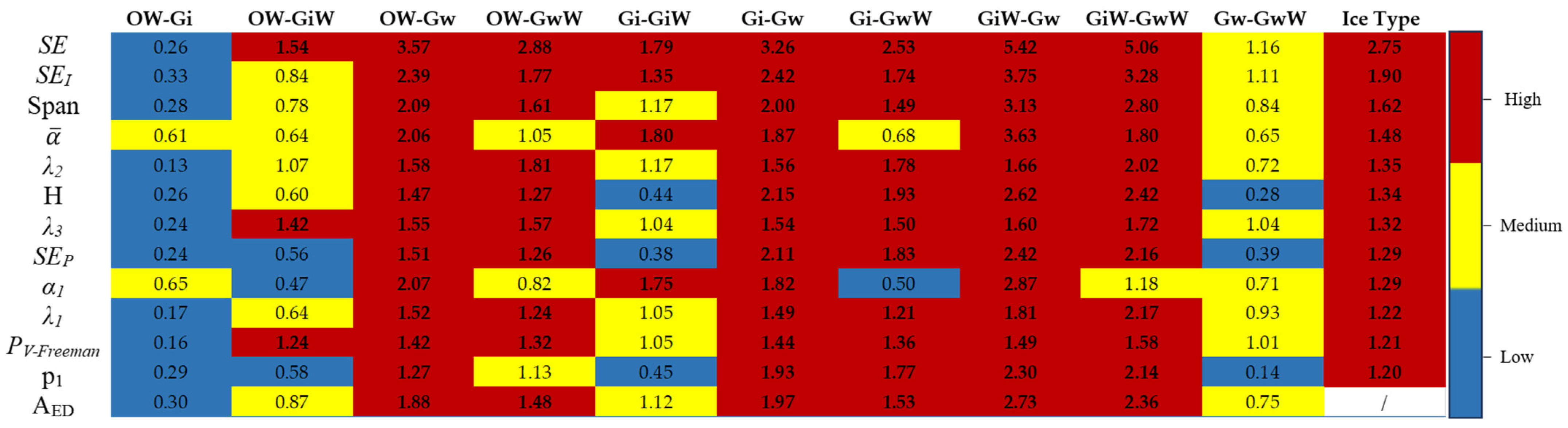
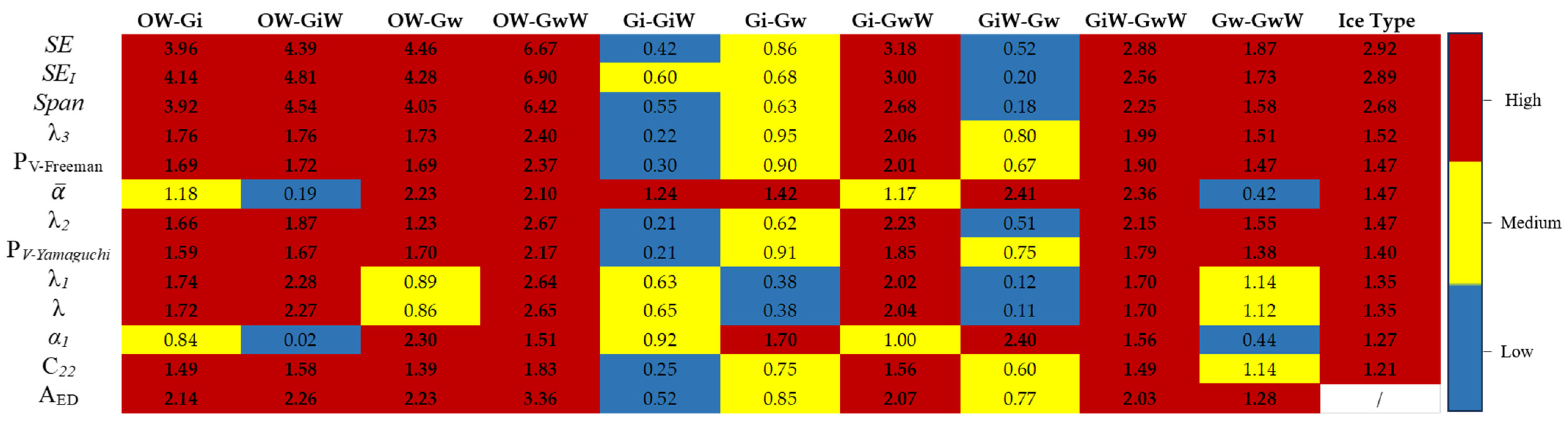
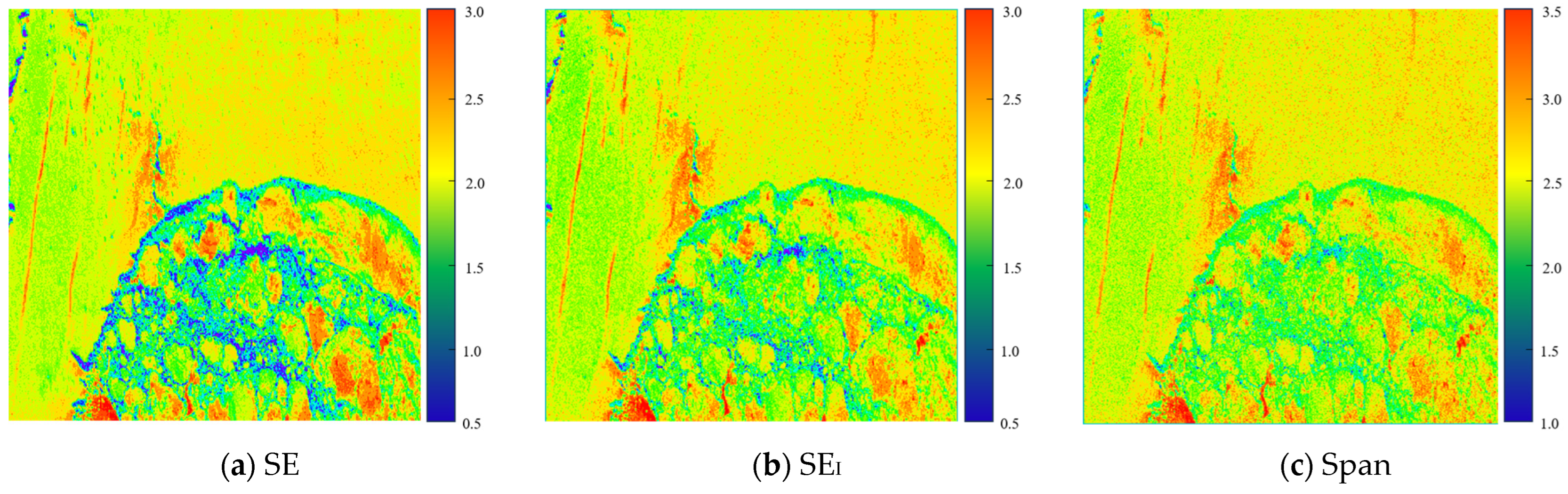
In the L-band, there are a total of 12 polarimetric features with Ice Type values greater than or equal to 1.2, with SE showing the highest sea-ice classification capability, having an Ice Type value of 2.75. The specific values of ED for these 12 polarimetric features in different classification combinations can be found in Figure 5, and the polarimetric feature images with the top three Ice Type values are displayed in Figure 6.

Observing Figure 6, it is evident that different types of sea ice exhibit distinct textures. Especially, the contrast between the rough surface of Gw and the smooth surface of Gi is quite clear. Using L-band polarization features provides an advantage in classifying sea ice with significant differences in surface roughness, which is consistent with previous research [38]. As shown in Figure 5, among these 10 type combinations, the A_ED values satisfying strong separability include OW–Gw, OW–GwW, Gi–Gw, Gi–GwW, GiW–Gw, and GiW–GwW. This indicates a relatively strong separability associated with Gw and GwW. However, L-band polarization features do not exhibit good separability in all sea-ice type combinations. For instance, the A_ED value for the Gw–GwW combination is 0.75, and none of the features meet the classification criteria, indicating poor separability between the two. Although Gw and GwW exhibit distinct brightness characteristics in optical imagery, in L-band SAR images, their backscattering coefficients are similar. The physical reason could be that GwW and Gw share similar physical structures, with rough surfaces and many cracks. Although GwW has some surface meltwater, it is minimal, and L-band electromagnetic waves are less sensitive to it.

While L-band polarization features exhibit strong separability in most sea-ice types, they perform poorly in separating thin ice (Gi and GiW) from open water (OW). The A_ED for OW–Gi and OW–GiW combinations in L-band polarization features is low, at only 0.30 and 0.87, respectively. The A_ED value for OW–Gi is the lowest among all type combinations, with all feature ED values below 1.2. This is because L-band frequencies are shorter, and electromagnetic waves have strong penetration capabilities [39], while Gi is relatively thin. In the feature image, the numerical values for OW and Gi are very close, resulting in poor separability. The same reasoning can explain the poor separability between OW and GiW. In conclusion, L-band polarization features perform poorly in classifying thin ice types [26,40], but they perform well in combinations with significant differences in thickness and roughness, such as Gi–Gw, Gi–GwW, GiW–Gw, and GiW–GwW.

4.1.2. S-Band

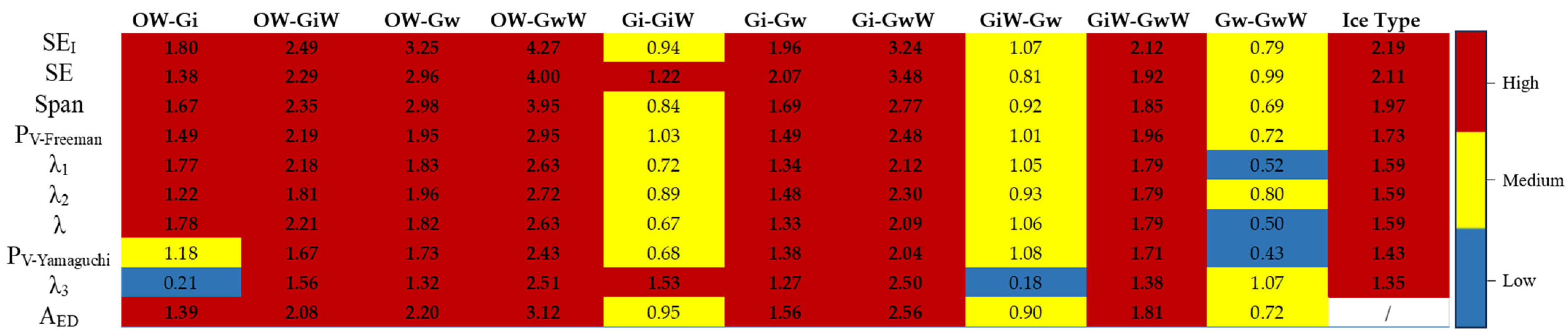
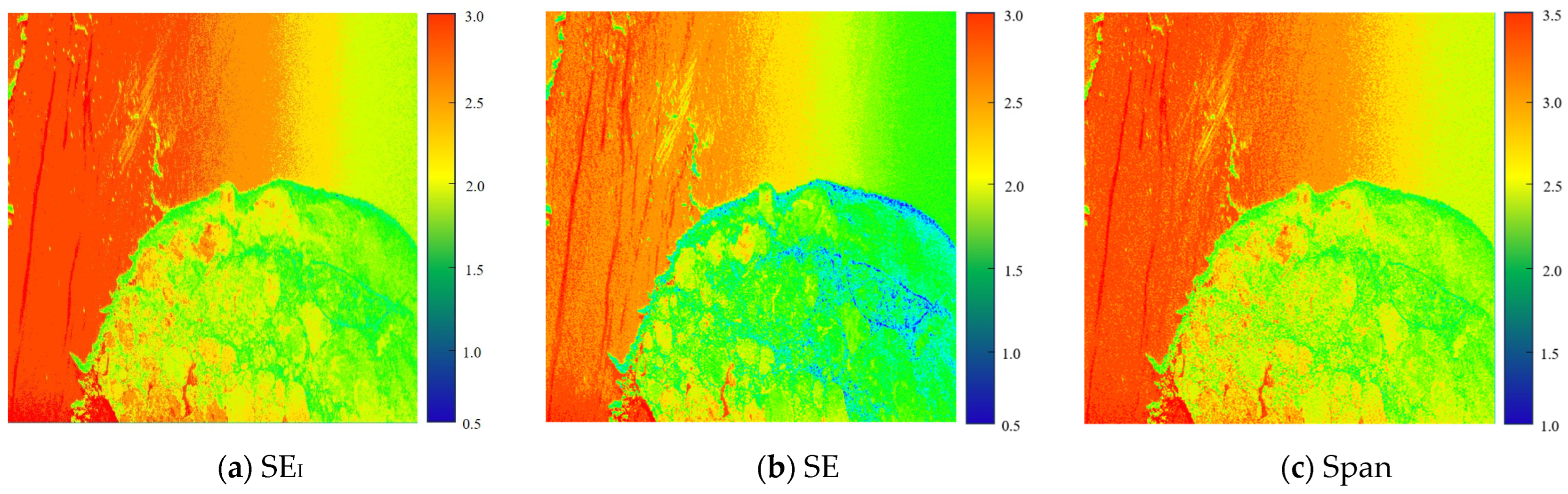
In the S-band, there are a total of nine polarimetric features that meet the classification criteria, with SE_I exhibiting the highest ice classification capability, having an Ice Type value of 2.19. The specific ED values of the polarimetric features that meet the classification criteria in various classification combinations are shown in Figure 7, and the polarimetric feature images with the top three Ice Type values are displayed in Figure 8.

Observing Figure 8a, it can be seen that seawater has the highest values in the Shannon entropy image, followed by Gi and GiW, while Gw and GwW have the lowest and closest values. Visually, there are distinct differences between seawater and sea ice. S-band polarization features perform well in the four combinations of sea ice and seawater (OW–Gi, OW–GiW, OW–Gw, OW–GwW). Specifically, the S-band polarization features meet the classification requirements for A_ED in these four combinations. Moreover, except for P_V-Yamaguchi and λ₃ in the OW–Gi combination, the ED values for S-band polarization features are greater than 1.2 in all four combinations.

Among the sea-ice type combinations, the A_ED values for S-band polarization features are less than 1.2 in the Gi–GiW, GiW–Gw, and Gw–GwW combinations. Particularly in the Gw–GwW combination, the ED values for all features are less than 1.2. But in the Gi–Gw, Gi–GwW and GiW–GwW combinations, the ED values for all features are more than 1.2. S-band performs better in the separability of thinner sea ice compared to other bands.

4.1.3. C-Band

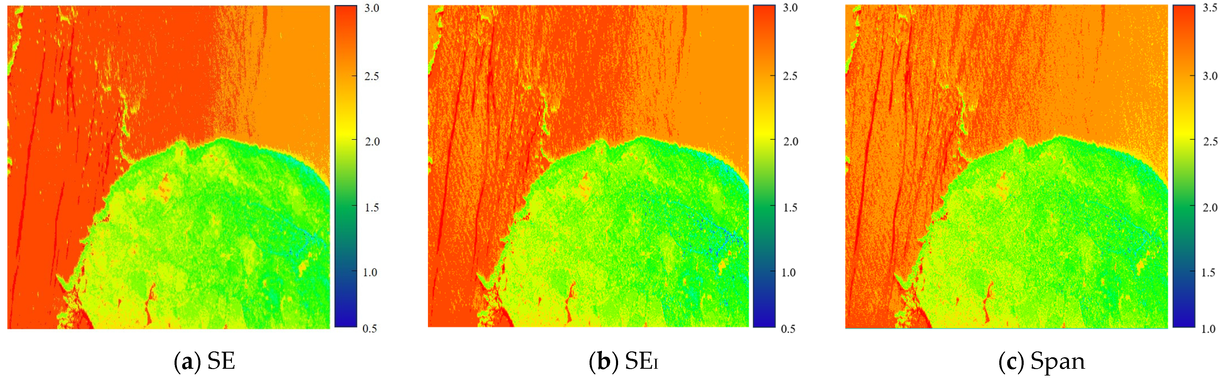
In the C-band, there are a total of 12 polarimetric features that meet the classification criteria, with SE exhibiting the highest ice classification capability, having an Ice Type value of 2.92. The specific ED values of the polarimetric features that meet the classification criteria in various classification combinations are shown in Figure 9, and the polarimetric feature images with the top three Ice Type values are displayed in Figure 10.

Observing Figure 10, we find that in the C-band polarization feature images, the numerical values for all types of sea ice are close, but there are significant differences compared to seawater. This is because the C-band radar wavelength is short, and seawater exhibits relatively high radar wave absorption in this frequency band. Seawater forms a strong contrasting state with sea ice, leading to clear differentiation between the two [41].

From Figure 9, we can see that the A_ED for all four combinations of sea ice and seawater is greater than 2 in the C-band. The numerical values in the C-band for these four combinations are higher than those in the S-band, indicating a stronger capability for distinguishing sea ice from seawater in the C-band. However, compared to other bands, C-band polarization features exhibit poorer separability among different sea-ice types. For example, in the Gi–GiW, Gi–Gw, and GiW–Gw combinations, the A_ED values for the selected polarization features are all less than 1. Particularly in the Gi–GiW combination, the A_ED is only 0.52, the lowest among all combinations, and only $\overline{\alpha }$ has an ED value greater than 1.2 in this combination. However, C-band features perform well in the Gi–GwW, GiW–GwW, and Gw–GwW combinations, with A_ED values all exceeding 1.2. Considering the A_ED value for the OW–GwW combination, we can conclude that in the C-band, GwW exhibits strong separability from other sea-ice types.

In summary, the L-band polarization features exhibit strong separability when dealing with sea-ice types related to Gw and GwW. However, their ability to distinguish between seawater and sea ice, especially in combinations with thin ice, is relatively weak. The S-band polarization features perform better in distinguishing between seawater and sea ice compared to the L-band but not as effectively as the C-band. They excel in separability, particularly in the case of thin ice. On the other hand, C-band polarization features show strong separability between seawater and sea ice, but there is still room for improvement in separability among different sea-ice types. In conclusion, the L-band is suitable for sea-ice type classification, the S-band is suitable for identifying thin ice types, and the C-band is suitable for sea-ice–water classification. This is consistent with the conclusion proposed by Dierking W, suggesting that higher-frequency electromagnetic waves are more reliable for sea-ice classification during the melting and freezing periods [42]. It is evident that the frequency of electromagnetic waves has a significant impact on the separability of sea-ice types.

4.2. Analysis and Comparison of Multi-Frequency Features

In order to analyze the properties of polarization features in each frequency band, we have compiled a total of 15 polarization features that meet the classification requirements. These features are as follows: λ₁, λ₂, λ₃, P₁, H, λ, $\overline{\alpha }$, α₁, SE, SE_I, SE_P, P_V-Freeman, P_V-Yamaguchi, C₂₂, and Span.

Through an analysis of the scattering mechanisms of the aforementioned polarization features, they can be broadly categorized into three groups:

(1)

Total power parameters (λ, SE, SE_I, SE_P, Span);

(2)

Volume scattering parameters (P_V-Freeman, P_V-Yamaguchi);

(3)

Scattering mechanism parameters (λ₁, λ₂, λ₃, P₁, H, $\overline{\mathsf{\alpha }}$, α₁, C₂₂).

In the three bands, there are seven common features that exhibit strong discriminative capabilities. These features are SE, SE_I, Span, λ₁, λ₂, λ₃, and P_V-Freeman. When ranking the discriminative capabilities of these features based on their Ice Type values in each frequency band, the top three features are consistently SE, SE_I, and Span. This is in line with the results discussed by Zhao et al. [43] regarding the importance of polarimetric features in sea-ice classification. The order of these features varies slightly between different frequency bands (with SE > SE_I > Span in L-band and C-band, and SE_I > SE > Span in the S-band). This suggests that features related to total power play a significant role in the classification of melting sea ice. The physical properties and structures of sea ice are closely related to their interaction with microwave signals, which are reflected in features related to power. Additionally, these parameters have a relatively lower dimensionality, making them simpler and more manageable in the feature space, facilitating easier processing and analysis.

The eigenvalues (λ_i (i = 1,2,3)) in the scattering mechanism parameters not only reflect the intensity of different scattering mechanisms on the Earth’s surface but also capture all the scattering information in the received echoes. Rich information can provide better classification capabilities, and the calculation of many scattering mechanism parameters is related to the eigenvalues λ_i, highlighting the significance of these eigenvalues.

Although the scattering mechanisms of sea ice typically involve surface scattering and volume scattering, we observed that the surface scattering parameters in the three bands do not show strong sea-ice classification ability. Furthermore, in the case of sea ice during the melting period, the classification performance of volume scattering parameters was significantly better than that of surface scattering parameters. This is attributed to the presence of meltwater on the ice surface during the melting process, which enhances microwave absorption and, in turn, complicates surface scattering characteristics, making them more difficult to distinguish [44]. In contrast, volume scattering parameters typically reflect the structural features inside the target, making them more suitable for distinguishing sea ice during the melting period. The two volume scattering parameters selected in this study are derived from Freeman decomposition and Yamaguchi decomposition. In all three bands, the separability of the volume scattering component features obtained from Freeman decomposition exceeded those obtained from Yamaguchi decomposition. This is because the volume scattering modeling in Freeman decomposition follows a random distribution, resulting in a more uniform numerical distribution of sea ice. In contrast, the volume scattering model in Yamaguchi decomposition is based on a sinusoidal distribution and introduces new helical scattering. Therefore, in the sea-ice data during the melting period in this experiment, the volume scattering energy in Freeman decomposition is greater than that in Yamaguchi decomposition, making the differences in volume scattering between different types of sea ice more pronounced and enhancing separability [45].

The above seven polarimetric features perform well in all three bands, indicating that these features are not significantly affected by the differences in electromagnetic wave frequencies, or the impact is relatively low when it comes to sea-ice classification.

The alpha approximation ($\overline{\mathsf{\alpha }}$) demonstrates good separability in both the L-band and the C-band. The calculation formula for $\overline{\mathsf{\alpha }}$ is closely related to parameters P₁ and α₁ [17], and these three parameters exhibit strong separability in the L-band. The stronger the difference in the shape of sea ice, the better the separability of $\overline{\mathsf{\alpha }}$. This is consistent with its performance in the separability of type combinations in the L-band and C-band, such as in the L-band, where $\overline{\mathsf{\alpha }}$ has A_ED values of 2.06 and 3.63 in OW–Gw and GiW–Gw combinations, respectively. Additionally, due to the different information acquisition capabilities of the L-band and C-band in distinguishing sea ice from seawater, $\overline{\mathsf{\alpha }}$ exhibits strong classification abilities in both bands.

Scattering entropy (H) reflects the randomness of the scattering return from the target and the structure of the target. Similar to $\overline{\mathsf{\alpha }}$, the greater the difference in the structure of the target, the stronger the separability. Compared to other bands, L-band electromagnetic waves can provide more information about the internal structure of sea ice, which is why the L-band scattering entropy exhibits good classification capabilities among different sea-ice types.

C₂₂ exhibits good separability in the C-band. C₂₂ represents the amplitude information of the backscattering signal in VV polarization mode, reflecting the intensity and scattering characteristics of VV polarization waves in SAR images. The greater the depolarization of backscattering from sea ice, the easier it is to distinguish it from water because water’s backscattering is mainly influenced by surface scattering, resulting in typically lower cross-polarized responses [12]. It is precisely because C₂₂ exhibits strong separability in combinations of sea ice and seawater, thus meeting the classification requirements.

5. Sea-Ice Classification

In this section, we constructed single-frequency feature sets using the polarimetric features that meet the classification requirements from Section 4.1. The organization of features is shown in the following

Table 5. The single-frequency feature sets.

Band	Polarimetric Feature	Total
L-band	SE, SEI, Span, $\overline{\mathsf{\alpha }}$, λ2, H, λ3, SEP, α1, λ1, PV-Freeman, p1	12
S-band	SEI, SE, Span, PV-Freeman, λ1, λ2, λ, PV-Yamaguchi, λ3	9
C-band	SE, SEI, Span, λ3, PV-Freeman, $\overline{\mathsf{\alpha }}$, λ2, PV-Yamaguchi, λ1, λ, α1, C22	12

.

5.1. Single-Frequency Sea-Ice Classification

5.1.1. Single-Frequency Classifier Selection

These single-frequency feature sets were then input into four machine learning algorithms separately to compare the overall accuracy.

Table 6. Accuracy of sea-ice classification using different machine learning classifiers.

Classifier	Band	Overall Accuracy	Kappa Coefficient
SVM	L	73.04%	0.5747
	S	76.70%	0.6221
	C	85.64%	0.7674
ML	L	66.37%	0.4828
	S	72.47%	0.6078
	C	81.81%	0.7146
RF	L	69.91%	0.5416
	S	75.49%	0.6149
	C	85.58%	0.7628
BPNN	L	69.70%	0.5274
	S	75.37%	0.6211
	C	85.49%	0.7619

presents the overall accuracy achieved by combining single-frequency polarimetric features with different classifiers.

The results show that the SVM classification method outperforms other methods in terms of overall accuracy and Kappa coefficient in all three bands. Therefore, we choose the SVM classifier to discuss the composition of the optimal polarimetric feature set for each band. We obtained classification results by using the single-frequency polarimetric feature sets and the SVM classifier. We calculated the corresponding confusion matrices (shown in

Table 7. Confusion matrix table of L-band classification results (percentage).

Class	OW	Gi	GiW	Gw	GwW	Total
OW	81.54	20.24	33.52	0.00	0.19	55.10
Gi	10.84	64.93	15.70	0.36	10.96	17.38
GiW	7.39	5.82	50.11	0.33	0.38	11.99
Gw	0.16	3.26	0.21	68.85	22.97	7.94
GwW	0.07	5.75	0.46	30.45	65.50	7.59
Total	100	100	100	100	100	73.04

,

Table 8. Confusion matrix table of S-band classification results (percentage).

Class	OW	Gi	GiW	Gw	GwW	Total
OW	91.29	11.10	8.40	1.74	0.29	56.41
Gi	1.33	62.98	12.77	27.82	1.95	12.95
GiW	7.36	22.36	65.36	29.31	23.04	20.07
Gw	0.01	3.51	8.79	31.19	19.73	5.59
GwW	0.01	0.06	4.68	9.93	54.99	4.97
Total	100	100	100	100	100	76.70

and

Table 9. Confusion matrix table of C-band classification results (percentage).

Class	OW	Gi	GiW	Gw	GwW	Total
OW	99.54	0.16	0.31	0.02	0.02	58.62
Gi	0.03	69.17	17.96	26.08	5.01	13.72
GiW	0.19	12.35	63.29	0.96	6.57	10.82
Gw	0.01	14.07	3.04	67.10	25.76	9.61
GwW	0.24	4.25	15.40	5.84	62.64	7.23
Total	100	100	100	100	100	85.64

) to analyze the classification capabilities of different bands for various types of sea ice.

The “Total” column in the confusion matrix corresponds to the percentage of pixels classified as a certain class in the total sample, and the bottom-most column represents the overall accuracy. By comparing the three confusion matrices, we can observe that in the C-band, OW and Gi have the highest production accuracy, GiW has the highest production accuracy in the S-band, and Gw and GwW have the highest production accuracy in the L-band.

In the L-band, the cases where Gi and GiW are misclassified as OW are more pronounced. The A_ED value for the OW–Gi and OW–GiW combinations is less than 1.2, with a commission error of 20.24% for Gi being wrongly classified as OW and 33.52% for GiW. Combining optical images with classification results, it can be observed that the misclassified GiW regions are mainly concentrated in areas with a high degree of melting, where the brightness in optical images is low and similar to that of seawater. This indicates that the L-band has poor classification capability for thinner sea ice (Gi, GiW) and is susceptible to confusion with seawater, which is consistent with the conclusions discussed in Section 4.1.1. Although the misclassification between Gw and GwW is more noticeable, both of them can be well distinguished from OW and Gi. The classification accuracies for Gw and GwW are 68.85% and 65.50%, respectively, the highest among the three bands. The L-band is better suited for the classification of Gw and GwW sea ice, which have rough surfaces and complex internal structures.

In comparison to the L-band, the S-band shows improved production accuracy for OW and GiW, but its accuracy for Gw decreases significantly, with a classification accuracy of only 31.19%. Gw is often misclassified as Gi and GiW, with commission errors of 27.82% and 29.31%, respectively. In Section 4.1.2, we discussed that S-band polarimetric features perform well in the Gi–Gw, Gi–GwW, and GiW–GwW combinations, with commission errors for these combinations all below 5%. This observation supports the earlier conclusion. The S-band, with a wavelength situated between the L-band and C-band, exhibits relatively balanced performance in classification, with an overall accuracy lying between that of the two bands.

OW exhibits the highest production accuracy in the C-band. Combining the production accuracies of OW in the L-band and S-band, we can observe that using shorter-wavelength bands results in higher classification accuracy for OW. In the C-band, the A_ED value for the OW–Gi combination is 2.14, with commission errors for Gi and Gw being only 0.03% and 0.16%, respectively. The A_ED for the Gi–Gw combination is 0.85, with Gi being misclassified as Gw at an error rate of 14.07%, and Gw being misclassified as Gi at an error rate of 26.08%. While the C-band does not exhibit the highest production accuracy for GwW, it is only slightly lower than the L-band.

To summarize, the commission error for various type combinations within each band is consistent with the separability findings outlined in Section 4.1. Essentially, combinations with low separability demonstrate noticeable commission errors, whereas combinations with high separability result in minimal commission errors.

5.1.2. Single-Frequency Classification Results

In order to discuss the composition of the optimal feature sets for each band and reduce data redundancy, we input the feature sets for each band into an SVM classifier and sequentially reduce the number of input features (N) using the RFE method. We then compare the classification accuracy at different numbers of features. The partial classification results for each wavelength band, shown in Figure 11 and Figure 12, illustrate the classification accuracy of the five sea-ice types across different wavelength bands and feature counts.

Figure 12a–c illustrate the production accuracy trends for L-band, S-band, and C-band classifications, respectively, while Figure 12d depicts the overall single-frequency classification accuracy trend. The x axis represents the number of features in the dataset, with an upper limit corresponding to the dimension of the respective polarization feature set. The y axis represents the production accuracy. These trend graphs are valuable for comprehending the connection between the number of features and production accuracy as well as the overall accuracy for a specific feature count and sea-ice type.

Combining Figure 11 and Figure 12, it can be observed that when N = 1, the overall accuracy for all three bands is relatively low, and achieving high accuracy with a single feature is currently challenging. As the number of features increases, the user accuracy for most sea-ice types improves to varying degrees. For example, in the C-band, when N = 5, the production accuracy for Gw is only 23.60%, but when N = 6, the production accuracy reaches 65.51%, marking an improvement of 41.91%. The feature introduced at this point is $\overline{\mathsf{\alpha }}$ which exhibits strong separability in the Gi–Gw combination with an ED value of 2.41. Its strong separability contributes to the overall accuracy improvement. Simultaneously, there are cases where production accuracy decreases with an increase in the number of features. In the L-band, for instance, the production accuracy for OW decreases from an initial 91.40% to a minimum of 80.10% as the number of features increases. This decrease in accuracy is attributed to the fact that OW’s backscatter coefficient in the L-band is close to the baseline noise and exhibits different regions in different polarization feature images. As the number of features increases, this effect becomes more pronounced, leading to decreasing production accuracy. When N is greater than 6, the overall accuracy trends in the L-band and C-band are not very significant, with variations typically remaining within approximately 1‰.

According to Figure 12d, the highest overall classification accuracies for the L-band, S-band, and C-band are 73.56%, 77.74%, and 85.74%, respectively. When each band achieves its highest classification accuracy, the corresponding number of features in the polarization feature set are 9, 6, and 6 for the L-, S-, and C-band, respectively. Based on this, the composition of the optimal polarization feature sets for each band is detailed in

Table 10. The optimal single-frequency feature sets.

Band	Polarimetric Feature	Total
L-band	SE, SEI, Span, $\overline{\mathsf{\alpha }}$, λ2, H, λ3, SEP, α1	9
S-band	SEI, SE, Span, PV-FREEMAN, λ1, λ2	6
C-band	SE, SEI, Span, λ3, PV-FREEMAN, $\overline{\mathsf{\alpha }}$	6

.

By comparing the overall accuracy of each band, we found that although the L-band has higher classification accuracy for Gw and GwW, its overall accuracy is lower than that of the S-band and C-band. “Overall” means that errors have been added for all types, so the ice conditions have some impact on the overall accuracy [42]. In this experimental scenario, Scene 1, experts statistically interpreted various types of sea ice in the image, with the proportion of seawater samples accounting for 58.83%, and other types accounting for about 10%. The classification accuracy of OW has the highest contribution to the overall accuracy, so the high production accuracy of the C-band for OW gives it a higher overall accuracy.

5.2. Multi-Frequency Sea-Ice Classification

5.2.1. Multi-Frequency Classifier Selection

Selecting one or more features directly related to the classification performance of classifiers is crucial in determining the best classifier–feature combination for ice classification [46]. Therefore, to assess the performance differences of these combinations, it is essential. We arrange the optimal polarimetric feature sets for each band in descending order according to the Ice Type values to form multi-dimensional polarimetric feature sets. Similarly, we employ the RFE method to explore the combinations of different classification methods using the best feature sets, where N is greater than or equal to 3. The classification accuracy of different classifier–feature combinations is displayed in Figure 13.

By observing Figure 13, we can see that the number of features required and their corresponding classification accuracy for different classifiers to achieve the highest overall accuracy are as follows: when using the ML classifier, 14 features are needed, with a classification accuracy of 91.12%; when using the SVM classifier, 12 features are needed, with a classification accuracy of 94.55%; when using the RF classifier, 15 features are needed, with a classification accuracy of 95.84%; when using the BPNN classifier, 15 features are needed, with a classification accuracy of 94.83%. This indicates that the RF classifier achieves the highest overall accuracy.

With the continuous increase in the number of features in Figure 13, except for the ML classifier, the classification accuracy of other classifiers improves to varying degrees. When N exceeds 12, other classifiers exhibit a decreasing trend in classification accuracy or a relatively stable classification accuracy. However, the RF classifier’s classification accuracy continues to improve and achieves the highest overall accuracy in this experiment. This advantage may be attributed to its suitability for handling large datasets compared to other classifiers [47].

5.2.2. Multi-Frequency Classification Results

In

Table 11. Each classifier corresponds to the composition of the optimal multi-dimensional polarization feature set.

Classifier	Polarimetric Features	Total
SVM	C-SE, C-SEI, L-SE, C-span, S-SEI, S-SE, S-span, L-SEI, S-PV-Freeman, L-span, S-λ1, S-λ2	12
ML	C-SE, C-SEI, L-SE, C-span, S-SEI, S-SE, S-span, L-SEI, S-PV-Freeman, L-span, S-λ1, S-λ2, C-λ3, L-$\overline{\mathsf{\alpha }}$	14
RF	C-SE, C-SEI, L-SE, C-span, S-SEI, S-SE, S-span, L-SEI, S-PV-Freeman, L-span, S-λ1, S-λ2, C-λ3, L-$\overline{\mathsf{\alpha }}$, C-PV-Freeman	15
BPNN	C-SE, C-SEI, L-SE, C-span, S-SEI, S-SE, S-span, L-SEI, S-PV-Freeman, L-span, S-λ1, S-λ2, C-λ3, L-$\overline{\mathsf{\alpha }}$, C-PV-Freeman, C-$\overline{\mathsf{\alpha }}$, C-λ2, S-PV-Yamaguchi, L-λ3	19

, we illustrate the composition of the optimal multi-dimensional polarimetric feature sets for each classifier. In this table, we use the term “band-feature” to indicate the wavelength range to which the features belong.

Even when using the same classifier, multi-dimensional polarimetric feature sets achieve higher classification accuracy with fewer features than single-frequency features. For example, with the SVM classifier, when N = 3, the multi-dimensional polarimetric feature set achieves an overall accuracy of 93.39%, significantly higher than the highest single-frequency overall accuracy of 85.74%. When compared to the highest classification accuracy in the three bands, the classification accuracy of the optimal multi-dimensional polarimetric feature set can be improved by 9% to 22%. The optimal multi-dimensional polarimetric feature set combines the excellent performance of the C-band in ice–water discrimination and the L-band in classifying ice types, resulting in a higher overall accuracy.

6. Validation and Comparison

6.1. Generalized Performance Verification

To ensure that the new sea-ice classification method based on feature selection from multi-dimensional SAR observational data proposed in this paper is equally applicable to other scenes, we selected four additional scenes for result comparison and validation. Among them, Scene 5, which has a different collection location and date from Scene 1, was chosen for single-band classification results and for comparing the selection of multi-band features and classifiers. The other three scenes were used to validate the feasibility of the method.

We utilized the data from Scene 5 to extract the polarimetric features listed in Table 5. The single-band polarimetric feature set was employed to obtain classification results, and confusion matrices were calculated. Figure 14 illustrates the variation in overall classification accuracy of the single-band feature set as N decreases.

Observing Figure 14d, we find that, unlike Scene 1, in Scene 5, the overall classification accuracy using the L-band feature set is the highest. This is because the classification accuracy is related to the number of sea-ice samples in the data, and in Scene 5, the number of sea-ice samples is much higher than that of seawater. Therefore, the L-band has higher classification accuracy among sea-ice classes compared to the C-band, resulting in higher overall classification accuracy. However, by observing Figure 14a–c, we can see that the classification capabilities of single-band feature sets among different sea-ice types are consistent with Scene 1. Specifically, OW and Gi have the highest classification accuracy in the C-band, GiW has the highest classification accuracy in the S-band, and Gw and GwW have the highest classification accuracy in the L-band. Moreover, the number of features required to achieve the highest classification accuracy in each band is consistent with Scene 1. Therefore, we can consider the single-band optimal feature set discussed in this study to be applicable to some extent.

Based on the arrangement of all features in the single-band feature set in Table 10, sorted in descending order of A_ED, we constructed a multi-band feature set. This multi-band feature set was sequentially input into different classifiers, and the classification results under different feature scenarios were discussed. The variation in overall classification accuracy is illustrated in Figure 15.

From Figure 15, it can be observed that the RF classifier also achieved the highest classification accuracy. Applying the corresponding feature sets from Table 11 to other scene data and using different classifier–feature combinations, the classification results are shown in Figure 16. In all four scenes, the highest classification accuracy is achieved using the RF classifier, with accuracies of 91.74%, 89.74%, 92.84%, and 93.4%. Therefore, the proposed method in this study can achieve high-precision classification of sea ice during the melting period in the Bohai Sea.

6.2. Comparison of Other Methods

We simulated Sentinel-1 satellite’s HH + HV dual-polarization data using C-band data and ALOS-2’s HH + HV dual-polarization data using L-band data. There are two scenes, namely Scene 1 and Scene 5. Additionally, we employed full-polarization data from the C-band and applied the classification methodology from a previous study on Bohai Sea ice classification [48]. The classification accuracy results for both scenes are shown in

Table 12. Dual-polarization data and previous research classification accuracy table.

Band	Polarization Mode	Scene	Overall Accuracy
L	HH + HV	Scene 1	58.57%
	HH + HV	Scene 5	63.68%
C	HH + HV	Scene 1	64.52%
	HH + HV	Scene 5	55.23%
	HH + HV + VH + VV	Scene 1	79.31%
	HH + HV + VH + VV	Scene 5	68.89%

.

By comparing the classification accuracy of dual-polarization data in Table 12 with the accuracy achieved using the multi-feature combinations discussed in this study, it is evident that the accuracy is higher with multi-band full-polarization data in different scenarios. This confirms the superiority of full-polarization data over using only dual-polarization data. The comparison with previous studies on C-band data further validates the feasibility of using multi-band data for sea-ice classification during the melting period.

7. Discussion and Conclusions

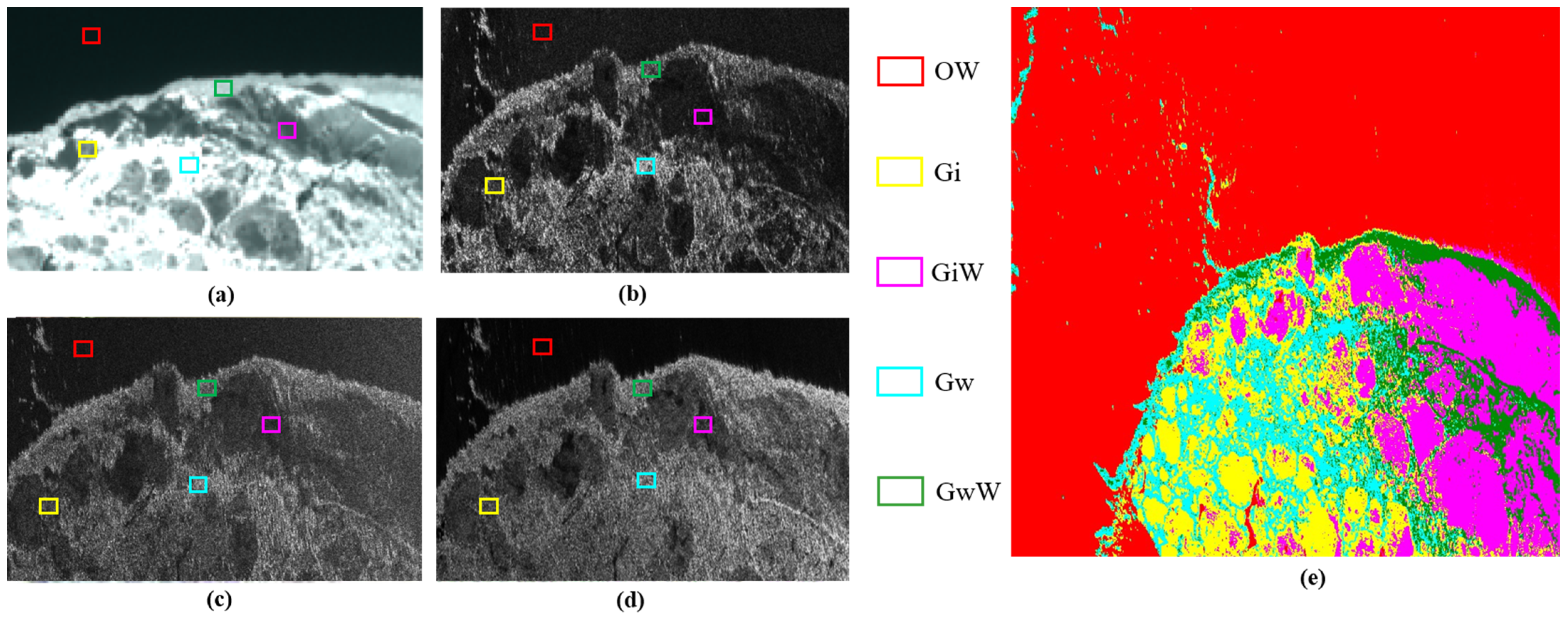
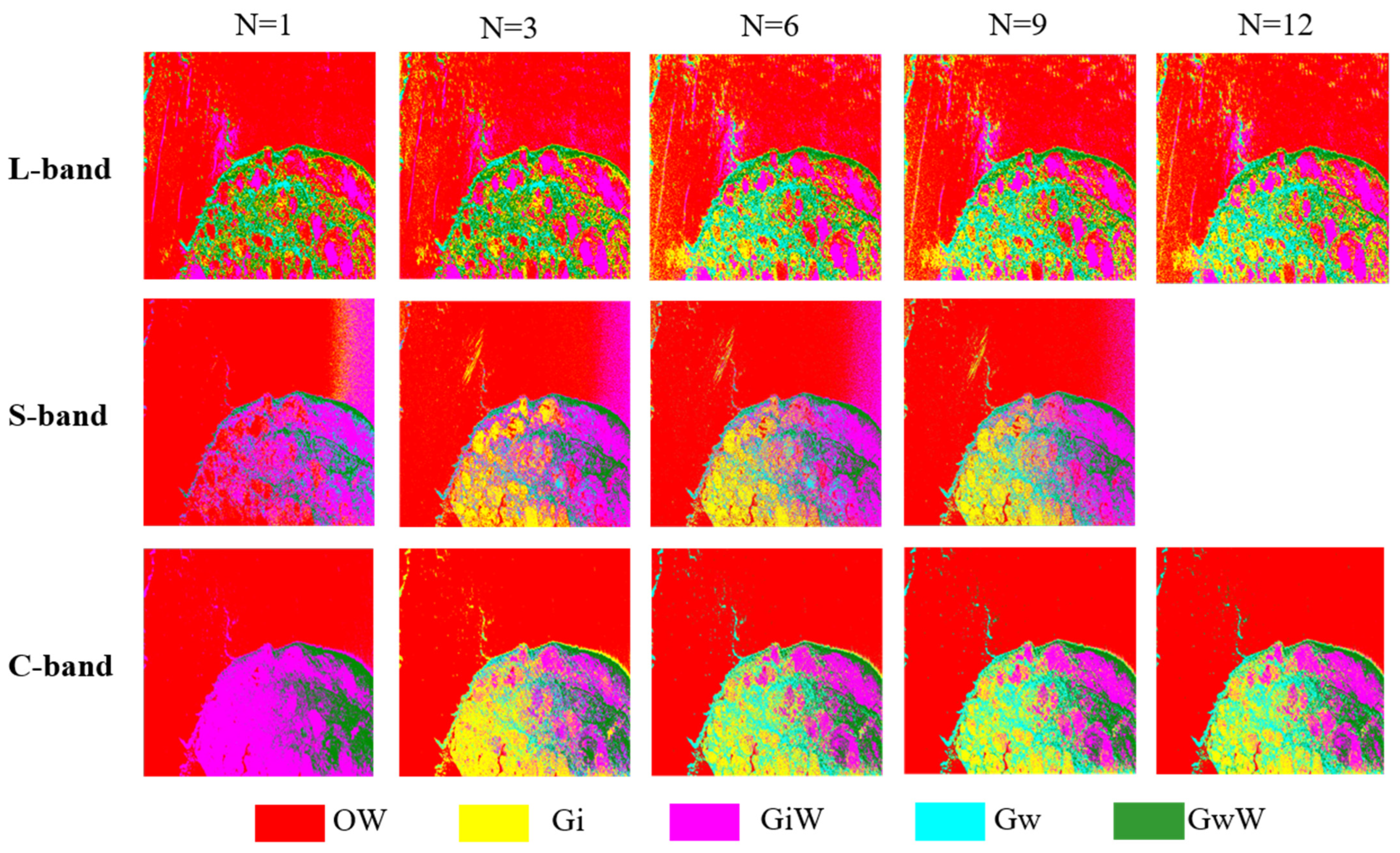
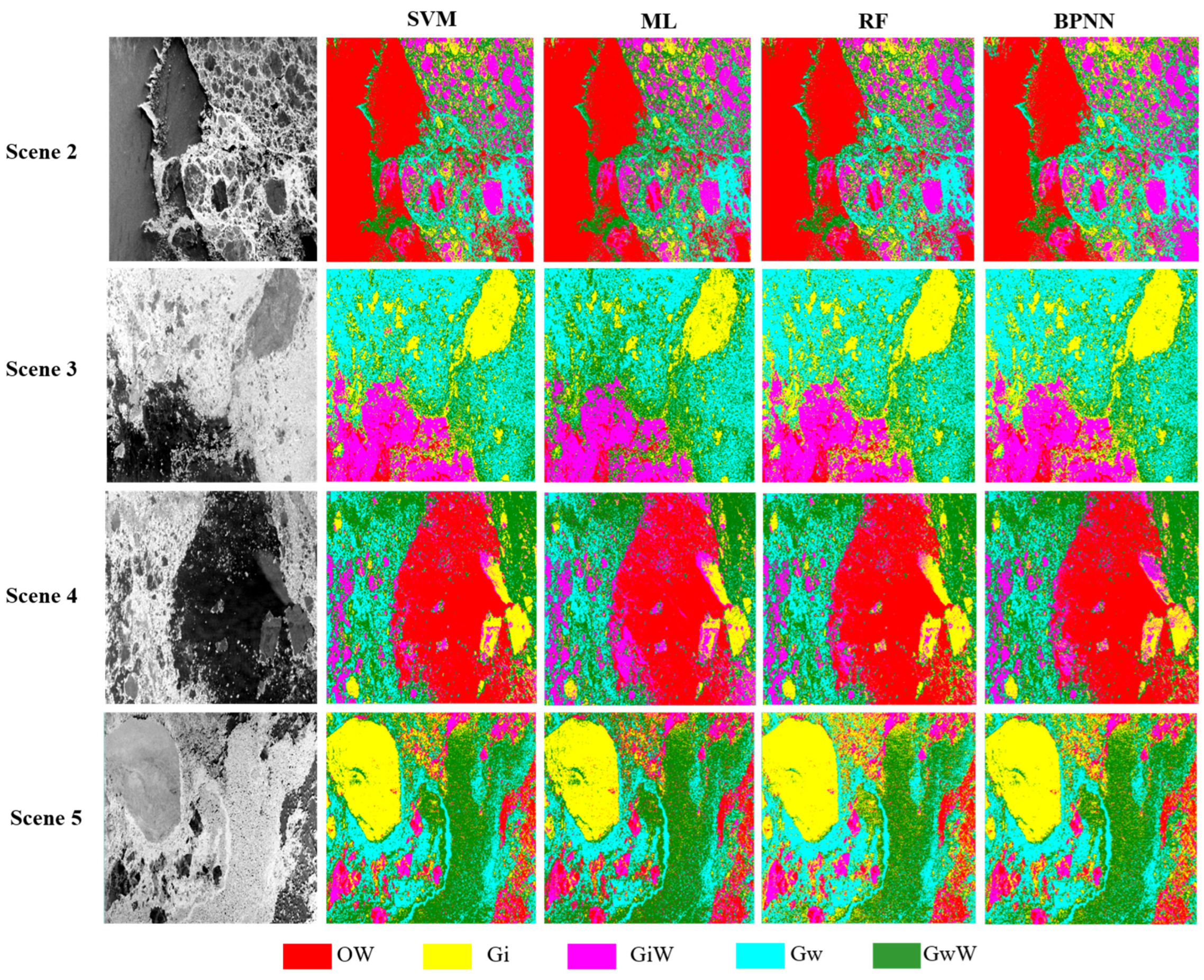
In this study, we proposed an ice classification method based on multi-dimensional SAR data feature selection. The new method was applied to the Bohai Sea and successfully classified OW, Gi, GiW, Gw, and GwW during the ice melting period.

To obtain multi-frequency, full-polarization PolSAR ice data during the ice melting season, the research team conducted a series of flight experiments over the Bohai Sea on 27–28 February 2022. They used a Modern Ark 60 aircraft equipped with a multi-dimensional SAR system and successfully acquired PolSAR data in the L-band, S-band, and C-band. This marked the first time that airborne SAR data were collected during the ice melting season in the Bohai Sea, providing valuable multi-frequency polarization data for ice research.

As the foundation of classification, the selection of polarization features is crucial. Firstly, we calculated the Euclidean distances between different types of sea ice and assessed the separability of 51 polarization features in the L-band, S-band, and C-band. The following conclusions were drawn: the L-band is suitable for ice type recognition, the S-band is suitable for classifying thin ice, and the C-band is suitable for ice–water classification. The results demonstrate that the L-band has 12 features, the S-band has 9 features, and the C-band has 12 features, totaling 33 polarization features with strong separability. Among them, SE, SE_I, and Span have shown outstanding performance in all three bands. Additionally, there are seven common polarization features that exhibit strong classification abilities in all three bands, and it is evident that volume scattering parameters are more suitable for classifying ice during the melting season than surface scattering parameters.

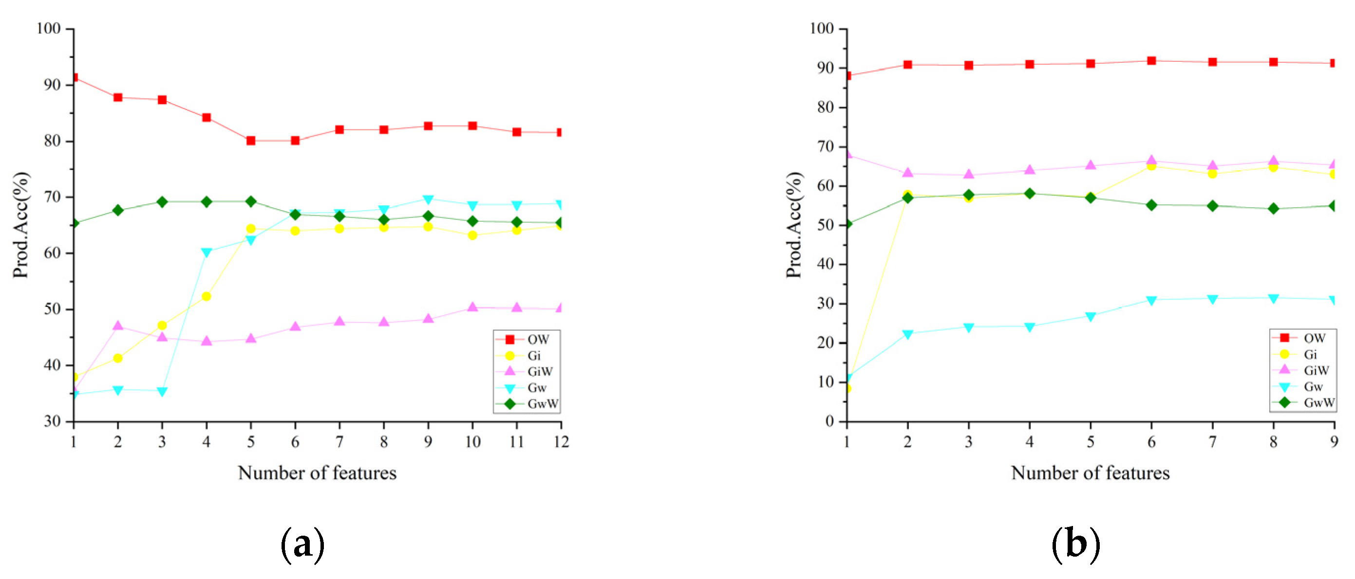
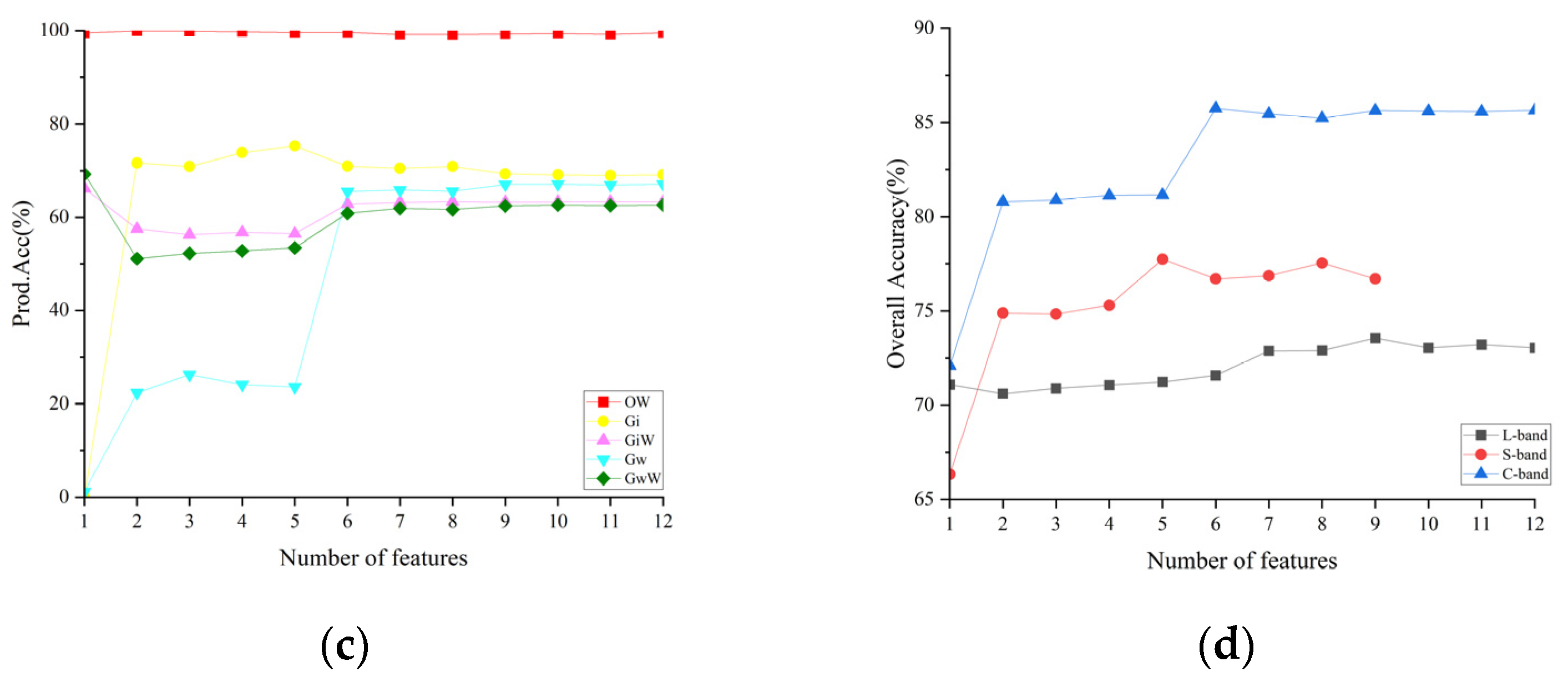
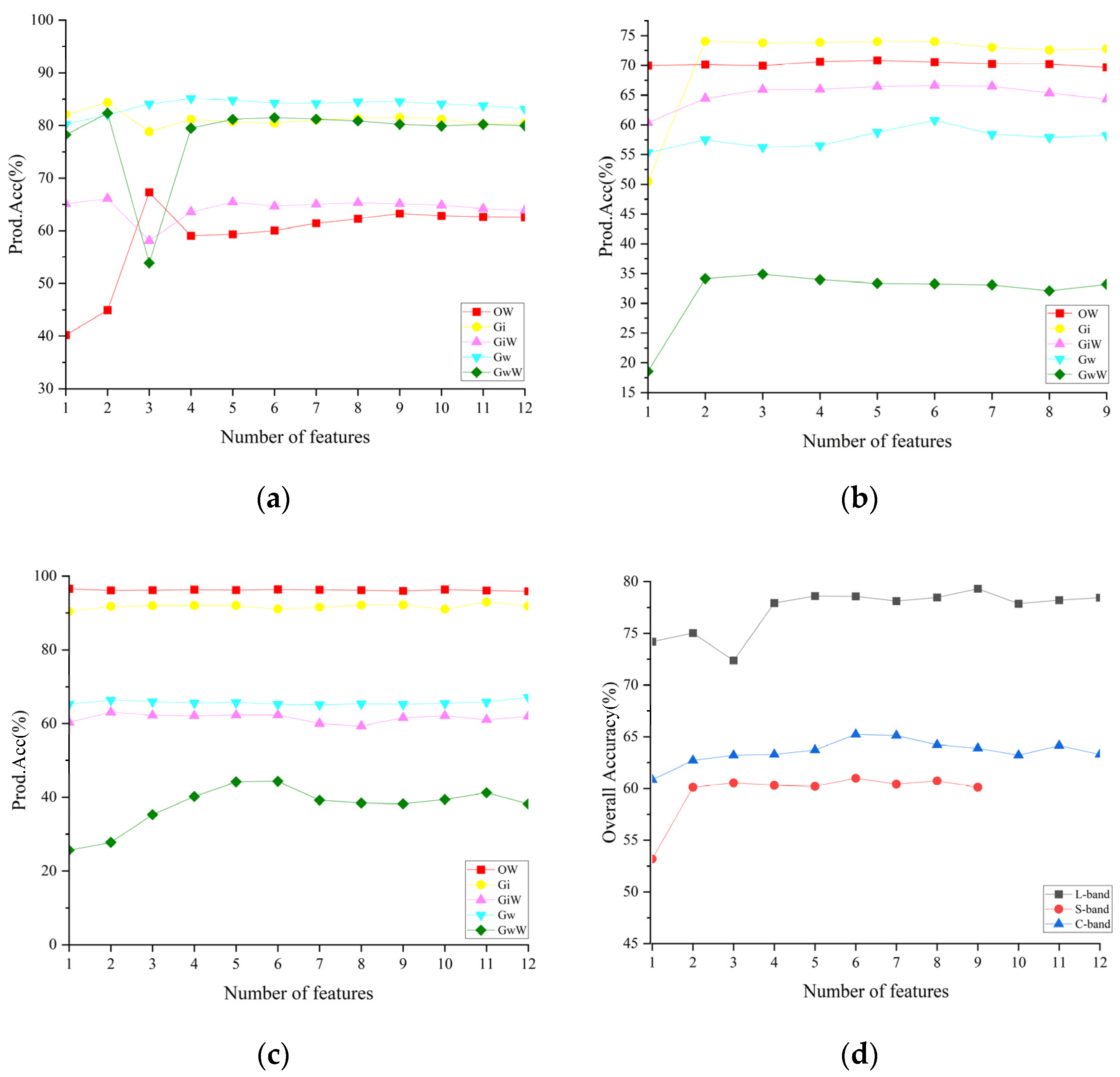
Furthermore, we constructed the eligible polarization features into polarization feature sets for each frequency band. Combining the RFE method, we input the feature sets into the SVM classifier and obtained classification results for different feature counts in each band. The results revealed that in the C-band, OW and Gi had the highest classification accuracy, GiW achieved the highest classification accuracy in the S-band, while Gw and GwW had the highest classification accuracy in the L-band. This can be attributed to the strong electromagnetic wave absorption of seawater at low frequencies. In the L-band images, the backscatter coefficient of seawater is lower, approaching the base noise level, resulting in lower classification accuracy for OW. Sea ice usually has a rough surface, and the L-band has better electromagnetic wave penetration capability, providing richer information about the internal structure of sea ice. Therefore, it achieves higher classification accuracy for rough sea-ice types like Gw and GwW, which is consistent with the findings in [35,36].

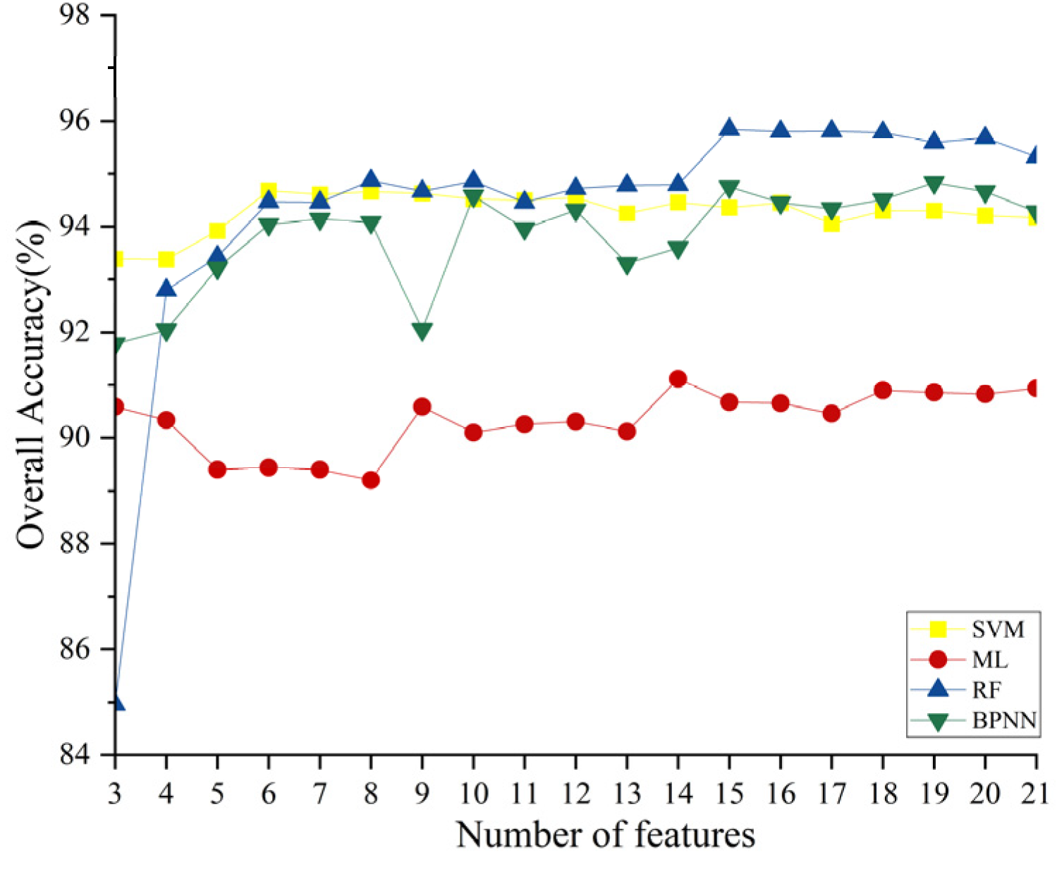
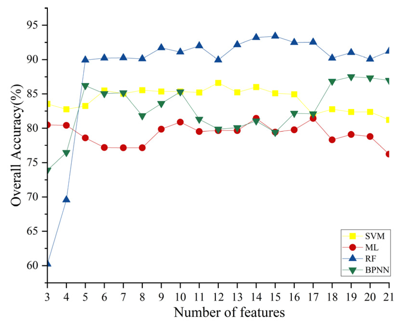
Finally, we utilized the SVM classifier to obtain single-frequency classification results and discussed the identification of the optimal single-frequency polarization feature set. We constructed a multi-dimensional polarization feature set by combining the optimal polarization features from the L-band, S-band, and C-band. Using the RFE method, we input these feature sets into four different machine learning classifiers. By comparing the ice classification accuracy at different feature counts, we discussed the composition of the optimal multi-dimensional SAR polarization feature set for different classifiers. In the case of using the SVM classifier, the multi-dimensional polarization feature set exhibited improved classification accuracy compared to the three single-frequency polarization feature sets, with improvements ranging from 9% to 22%. The highest classification accuracy among different feature–classifier combinations was achieved when using the RF classifier at 95.84%. We validated our proposed method using verification data, and the results similarly demonstrated that our method is effective for classifying sea-ice types OW, Gi, GiW, Gw, and GwW during the melting season in the Bohai Sea.

According to the experimental results in this paper, we observed that the SVM classifier achieves higher classification accuracy when using a single-band feature set. In this case, the feature set contains fewer features with strong data correlation, making SVM more robust in handling the data. When using a multi-band feature set, which contains more features than the single-band feature set and is more complex, the RF classifier’s accuracy is superior to other models. It is mentioned that RF is more suitable for handling complex datasets, which aligns with the conclusions drawn in our paper.

We verify the generalization performance of the model by using four-scene validation data. The results of the validation indicated that the classification accuracy exceeded 89.74% across various scenarios. Additionally, we simulated Sentinel-1’s HH + HV dual-polarization data using C-band data and ALOS-2’s HH + HV dual-polarization data using L-band data. The results demonstrate that the comprehensive use of full-polarization data is superior to using only dual-polarization data. The comparison with previous studies on C-band data further validates the feasibility of using multi-band data for sea-ice classification during the melting period.

It might be challenging to obtain multi-band synchronous satellite data for sea-ice classification. However, in regions with high-frequency satellite coverage, such as polar areas, it is possible to leverage data from multiple satellites to achieve near-real-time sea-ice classification. Sea-ice melting is a slow process, and with the continuous increase in satellite data in the future, a coordinated approach using near-real-time data from multiple satellites is a possibility. This study focuses on exploring the classification capabilities of different bands in sea-ice classification, and the conclusions drawn from single-band data can be applied to satellite data. The conclusions obtained from the multi-frequency data can be used as reference for the subsequent development of multi-frequency satellites.

In conclusion, the novel sea-ice classification method based on PolSAR observation data feature selection proposed in this study has effectively classified sea ice during the melting season in the Bohai Sea. Currently, many deep learning models are applied to sea-ice classification, and these models often require a large amount of data for support to achieve good results. However, obtaining synchronized data for multi-band full polarization is challenging, and the dataset in this study may be insufficient to support the use of such networks. The future direction of improvement for this work involves accumulating a large amount of multi-band data. This can be achieved by conducting more airborne SAR flight experiments while simultaneously collecting near-real-time data from areas with high-frequency satellite coverage, including data from C-band, L-band, and S-band satellites. Applying airborne remote sensing methods to satellite remote sensing can be beneficial for improving the accuracy of sea-ice classification during the melting period.

References

1. Mark, C.; Serreze, M.C.; Barry, R.G. Processes and impacts of Arctic amplification: A research synthesis. Glob. Planet. Chang. 2011, 77, 85–96. [Google Scholar] [CrossRef]
2. Su, H.; Wang, Y.; Xiao, J.; Li, L. Improving MODIS sea ice detectability using gray level co-occurrence matrix texture analysis method: A case study in the Bohai Sea. ISPRS J. Photogramm. Remote Sens. 2013, 85, 13–20. [Google Scholar] [CrossRef]
3. Gelis, I.D.; Colin, A.; Longepe, N. Prediction of Categorized Sea Ice Concentration from Sentinel-1 SAR Images Based on a Fully Convolutional Network. IEEE J. Sel. Top. Appl. Earth Obs. Remote Sens. 2021, 99, 5831–5841. [Google Scholar] [CrossRef]
4. Wang, M.; Shi, W. Detection of Ice and Mixed Ice–Water Pixels for MODIS Ocean Color Data Processing. IEEE Trans. Geosci. Remote Sens. 2009, 47, 2510–2518. [Google Scholar] [CrossRef]
5. Kim, J.-W.; Kim, D.-J.; Hwang, B.J. Characterization of Arctic Sea Ice Thickness Using High-Resolution Spaceborne Polarimetric SAR Data. IEEE Trans. Geosci. Remote Sens. 2012, 50, 13–22. [Google Scholar] [CrossRef]
6. Macdonald, R.W.; Harner, T.; Fyfe, J. Recent climate change in the Arctic and its impact on contaminant pathways and interpretation of temporal trend data. Sci. Total Environ. 2005, 342, 5–86. [Google Scholar] [CrossRef]
7. Casey, J.; Howell, S.E.; Tivy, A.; Haas, C. Separability of sea ice types from wide swath C- and L-band synthetic aperture radar imagery acquired during the melt season. Remote Sens. Environ. Interdiscip. J. 2016, 174, 314–328. [Google Scholar] [CrossRef]
8. Cavalieri, D.J. A microwave technique for mapping thin sea ice. J. Geophys. Res. Ocean. 1994, 99, 12561–12572. [Google Scholar] [CrossRef]
9. Dierking, W.; Skriver, H.; Gudmandsen, P. On the improvement of sea ice classification by means of radar polarimetry. In Remote Sensing in Transition; Alfred Wegener Institute for Polar and Marine Research: Bremerhaven, Germany, 2004. [Google Scholar]
10. Shang, F.; Hirose, A. Quaternion Neural-Network-Based PolSAR Land Classification in Poincare-Sphere-Parameter Space. IEEE Trans. Geosci. Remote Sens. 2014, 52, 5693–5703. [Google Scholar] [CrossRef]
11. Espeseth, M.; Brekke, C.; Johansson, A. Assessment of RISAT-1 and Radarsat-2 for Sea Ice Observations from a Hybrid-Polarity Perspective. Remote Sens. 2017, 9, 1088. [Google Scholar] [CrossRef]
12. De Abreu, R.; Flett, D.; Scheuchl, B.; Ramsay, B. Operational sea ice monitoring with RADARSAT-2—A glimpse into the future. In Proceedings of the 2003 IEEE International Geoscience and Remote Sensing Symposium, Toulouse, France, 21–25 July 2003; Volume 2, pp. 1308–1310. [Google Scholar] [CrossRef]
13. Kwon, T.J.; Li, J.; Wong, A. ETVOS: An Enhanced Total Variation Optimization Segmentation Approach for SAR Sea-Ice Image Segmentation. IEEE Trans. Geosci. Remote Sens. 2013, 51, 925–934. [Google Scholar] [CrossRef]
14. Zakhvatkina, N.Y.; Alexandrov, V.Y.; Johannessen, O.M.; Sandven, S.; Frolov, I.Y. Classification of Sea Ice Types in ENVISAT Synthetic Aperture Radar Images. IEEE Trans. Geosci. Remote Sens. 2013, 51, 2587–2600. [Google Scholar] [CrossRef]
15. Wang, T.; Yang, X.; Wang, Y.; Fang, J.; Jia, L. A multi-level SAR sea ice image classification method by incorporating egg-code-based expert knowledge. In Proceedings of the 2012 5th International Congress on Image and Signal Processing (CISP), Chongqing, China, 16–18 October 2012. [Google Scholar] [CrossRef]
16. Liu, M.; Dai, Y.; Zhang, J.; Ren, G.; Meng, J.; Zhang, X. Research on Sea Ice Secondary Classification Method Using High-Resolution Fully Polarimetric Synthetic Aperture Radar Data. Acta Oceanol. Sin. 2013, 4, 80–87. (In Chinese) [Google Scholar] [CrossRef]
17. Cloude, S.R.; Pottier, E. An entropy-based classification scheme for land applications of polarimetric SAR. IEEE Trans. Geosci. Remote Sens. 1997, 35, 68–78. [Google Scholar] [CrossRef]
18. Freeman, A.; Durden, S.L. A three-component scattering model for polarimetric SAR data. Trans. Geosci. Remote Sens. 1998, 36, 963–973. [Google Scholar] [CrossRef]
19. Yamaguchi, Y.; Moriyama, T.; Ishido, M.; Yamada, H. Four-component scattering model for polarimetric SAR image decomposition. IEEE Trans. Geosci. Remote Sens. 2005, 43, 1699–1706. [Google Scholar] [CrossRef]
20. Zhang, X. Polarimetric SAR Study on Bohai Sea Ice Thickness. Ph.D. Dissertation, Ocean University of China, Qingdao, China, 2011. (In Chinese). [Google Scholar]
21. Scheuchl, B.; Hajnsek, I.; Cumming, I.G. Model-based classification of polarimetric SAR sea ice data. In Proceedings of the IGARSS’02, Toronto, ON, Canada, 24–28 June 2002. [Google Scholar] [CrossRef]
22. Dabboor, M.; Geldsetzer, T.; Babelli, A. Towards sea ice classification using simulated RADARSAT Constellation Mission compact polarimetric SAR imagery. Remote Sens. Environ. 2014, 140, 189–195. [Google Scholar] [CrossRef]
23. Zhang, X.; Dierking, W.; Zhang, J.; Meng, J. A Polarimetric Decomposition Method for Ice in the Bohai Sea Using C-Band PolSAR Data. IEEE J. Sel. Top. Appl. Earth Obs. Remote Sens. 2015, 8, 47–66. [Google Scholar] [CrossRef]
24. Zhang, J.; Zhang, W.; Hu, Y.; Chu, Q.; Liu, L. An Improved Sea Ice Classification Algorithm with Gaofen-3 Dual-Polarization SAR Data Based on Deep Convolutional Neural Networks. Remote Sens. 2022, 14, 906. [Google Scholar] [CrossRef]
25. Zhang, T.; Yang, Y.; Shokr, M.; Mi, C.; Li, X.-M.; Cheng, X.; Hui, F. Deep Learning Based Sea Ice Classification with Gaofen-3 Fully Polarimetric SAR Data. Remote Sens. 2021, 13, 1452. [Google Scholar] [CrossRef]
26. Rignot, E.; Drinkwater, M.R. Winter sea ice mapping from multi-parameter synthetic aperture radar data. J. Glaciol. 1994, 40, 31–45. [Google Scholar] [CrossRef]
27. Xie, Q.; Lang, W.; Zhang, X.; Yang, X. On the improvement of sea ice classification by fusing C- and L-band SAR-C polarimetric quantities. In Proceedings of the International Conference on Intelligent Control & Information Processing, Beijing, China, 9–11 June 2013; Volume 12, pp. 103–107. [Google Scholar] [CrossRef]
28. Eltoft, T.; Doulgeris, A.P.; Grahn, J. Model-based polarimetric decomposition of Arctic sea ice. In Proceedings of the EUSAR 2014, 10th European Conference on Synthetic Aperture Radar, Berlin, Germany, 3–5 June 2014. [Google Scholar]
29. Li, D.; Wang, G.; Qin, C.; Wu, B. River Extraction under Bankfull Discharge Conditions Based on Sentinel-2 Imagery and DEM Data. Remote Sens. 2021, 13, 2650. [Google Scholar] [CrossRef]
30. GB/T 14914.2-2019; China National Standardization Management Committee. Specifications for Marine Observations. China Standards Publishing House: Beijing, China, 2019.
31. Tavri, A.; Scharien, R.; Geldsetzer, T. Melt Season Arctic Sea Ice Type Separability Using Fully and Compact Polarimetric C- and L-Band Synthetic Aperture Radar. Can. J. Remote Sens. 2023, 49, 2271578. [Google Scholar] [CrossRef]
32. Yu, H.; Wang, C.; Li, J.; Sui, Y. Automatic Extraction of Green Tide From GF-3 SAR Images Based on Feature Selection and Deep Learning. IEEE J. Sel. Top. Appl. Earth Obs. Remote Sens. 2021, 14, 10598–10613. [Google Scholar] [CrossRef]
33. Du, Y. Image Retrieval with Minimum Euclidean Distance and Relevant Feedback Based on Bayesian Classifier, and DSP Implementation. Master’s Dissertation, Jilin University, Changchun, China, 2006. (In Chinese). [Google Scholar]
34. Leigh, S.; Wang, Z.; Clausi, D. Automated ice–water classification using dual-polarization SAR satellite imagery. IEEE Trans. Geosci. Remote Sens. 2014, 52, 5529–5539. [Google Scholar] [CrossRef]
35. Liu, H.; Guo, H.; Zhang, L. SVM-Based sea ice classification using textural features and concentration from RADARSAT-2 Dual-Pol ScanSAR data. IEEE J. Sel. Top. Appl. Earth Obs. Remote Sens. 2015, 8, 1601–1613. [Google Scholar] [CrossRef]
36. Guyon, I.; Weston, J.; Barnhill, S.; Vapnik, V. Gene Selection for Cancer Classification using Support Vector Machines. Mach. Learn. 2002, 46, 389–422. [Google Scholar] [CrossRef]
37. Shamshiri, R.; Eide, E.; Hyland, K.V. Spatio-temporal distribution of sea-ice thickness using a machine learning approach with Google Earth Engine and Sentinel-1 GRD data. Remote Sens. Environ. 2022, 270, 112851. [Google Scholar] [CrossRef]
38. Pearson, D.; Livingstone, C.E.; Hawkins, R.K.; Gray, A.L.; Arsenault, L.D.; Wilkenson, T.L.; Okamoto, K. Radar detection of sea-ice ridges and icebergs in frozen oceans at incidence angles from 0 to 90. In Proceedings of the 6th Canadian Symposium on Remote Sensing, Halifax, NS, Canada, 21–23 May 1980. [Google Scholar]
39. Rott, H.; Domik, G.; Maetzler, C.; Miller, H. Study on Use and Characteristics of SAR for Land Snow and Ice Applications; Institut fur Meteorologie und Geophysik, Universität Innsbruck: Innsbruck, Austria, 1985. [Google Scholar]
40. Lee, J.S.; Grunes, M.; Kwok, R. Classification of multi-look polarimetric SAR imagery based on complex wishart distribution. Int. J. Remote Sens. 1992, 15, 2299–2311. [Google Scholar] [CrossRef]
41. Matsuoka, T.; Uratsuka, S.; Satake, M.; Kobayashi, T.; Nadai, A.; Umehara, T.; Maeno, H.; Wakabayashi, H.; Nakamura, K.; Nishio, F. CRL/NASDA airborne SAR (Pi-SAR) observations of sea ice in the sea of okhotsk. Ann. Glaciol. 2001, 33, 115–119. [Google Scholar] [CrossRef]
42. Dierking, W.; Busche, T. Sea ice monitoring by L-band SAR: An assessment based on literature and comparisons of JERS-1 and ERS-1 imagery. IEEE Trans. Geosci. Remote Sens. 2006, 44, 957–970. [Google Scholar] [CrossRef]
43. Zhao, Q.; Guo, S.; Li, X.; Li, Y. Sea ice classification in full polarimetric SAR using target decomposition features. Acta Geod. Cartogr. Sin. 2018, 47, 1609–1620. (In Chinese) [Google Scholar]
44. Sanden, J.J.V.D.; Drouin, H. Satellite SAR Observations of River Ice Cover: A RADARSAT-2 (C-band) and ALOS PALSAR (L-band) Comparison. In Proceedings of the 16th Workshop on River Ice, Winnipeg, MB, Canada, 18–22 September 2011. [Google Scholar]
45. Lee, J.S.; Pottier, E. Polarimetric Radar Imaging: From Basics to Applications; CRC Press: Boca Raton, FL, USA, 2009. [Google Scholar]
46. Shen, X.; Zhang, J.; Zhang, X.; Meng, J.; Ke, C. Sea Ice Classification Using Cryosat-2 Altimeter Data by Optimal Classifier-Feature Assembly. IEEE Geosci. Remote Sens. Lett. 2017, 11, 1–5. [Google Scholar] [CrossRef]
47. Lu, Y.; Zhang, B.; Perrie, W. Arctic Sea Ice and Open Water Classification from Spaceborne Fully Polarimetric Synthetic Aperture Radar. IEEE Trans. Geosci. Remote Sens. 2023, 61, 1–13. [Google Scholar] [CrossRef]
48. Zhang, X.; Zhang, J.; Liu, M.; Meng, J. Assessment of C-band compact polarimetry SAR for sea ice classification. Acta Oceanol. Sin. 2016, 35, 79–88. [Google Scholar] [CrossRef]
Figure 1. Map of study area in the vicinity of Bayuquan in Liaodong Bay. The coverage of PolSAR data is represented with red and yellow rectangles, and the coverage of Sentinel-2 images is delineated by the blue rectangle, and the black rectangle in the Bohai inset map shows the geographical location of the study area.
Remotesensing 16 01100 g001
Figure 3. (a) Sample examples of different sea-ice types in Sentinel-2 imagery, (b) L-band, (c) S-band, (d) C-band images in Scene 1; (e) expert interpretation map.
Remotesensing 16 01100 g003
Figure 4. Flowchart of sea-ice classification during melting period with multi-frequency PolSAR data.
Remotesensing 16 01100 g004
Figure 5. The Euclidean distance of L-band polarimetric features in different type combinations, the columns in the figure represent combinations of sea-ice types, with each row corresponding to a different polarimetric features and a different color indicating its divisibility.
Remotesensing 16 01100 g005
Figure 6. The top three polarimetric feature images with the highest classification capability in the L-band.
Remotesensing 16 01100 g006
Figure 7. The Euclidean distance of S-band polarimetric features in different type combinations, the columns in the figure represent combinations of sea-ice types, with each row corresponding to a different polarimetric features and a different color indicating its divisibility.
Remotesensing 16 01100 g007
Figure 8. The top three polarimetric feature images with the highest classification capability in the S-band.
Remotesensing 16 01100 g008
Figure 9. The Euclidean distance of C-band polarimetric features in different type combinations, the columns in the figure represent combinations of sea-ice types, with each row corresponding to a different polarimetric features and a different color indicating its divisibility.
Remotesensing 16 01100 g009
Figure 10. The top three polarimetric feature images with the highest classification capability in the C-band.
Remotesensing 16 01100 g010
Figure 11. The partial classification result images for Scene 1. Each row represents a different band, and each column represents the corresponding number of polarization features.
Remotesensing 16 01100 g011
Figure 12. (a) Single-band sea-ice production accuracy trend plot for L-band in Scene 1, (b) S-band, (c) C-band, (d) Overall single-band sea-ice classification accuracy plot.
Remotesensing 16 01100 g012aRemotesensing 16 01100 g012b
Figure 13. The overall accuracy trends for different classifiers in Scene 1.
Remotesensing 16 01100 g013
Figure 14. (a) Single-band sea-ice production accuracy trend plot for L-band in Scene 5, (b) S-band, (c) C-band, (d) Overall single-band sea-ice classification accuracy plot.
Remotesensing 16 01100 g014
Figure 15. The overall accuracy trends for different classifiers in Scene 5.
Remotesensing 16 01100 g015
Figure 16. Validation data and classification results; each row represents a different scene, and each column represents a different classifier.
Remotesensing 16 01100 g016